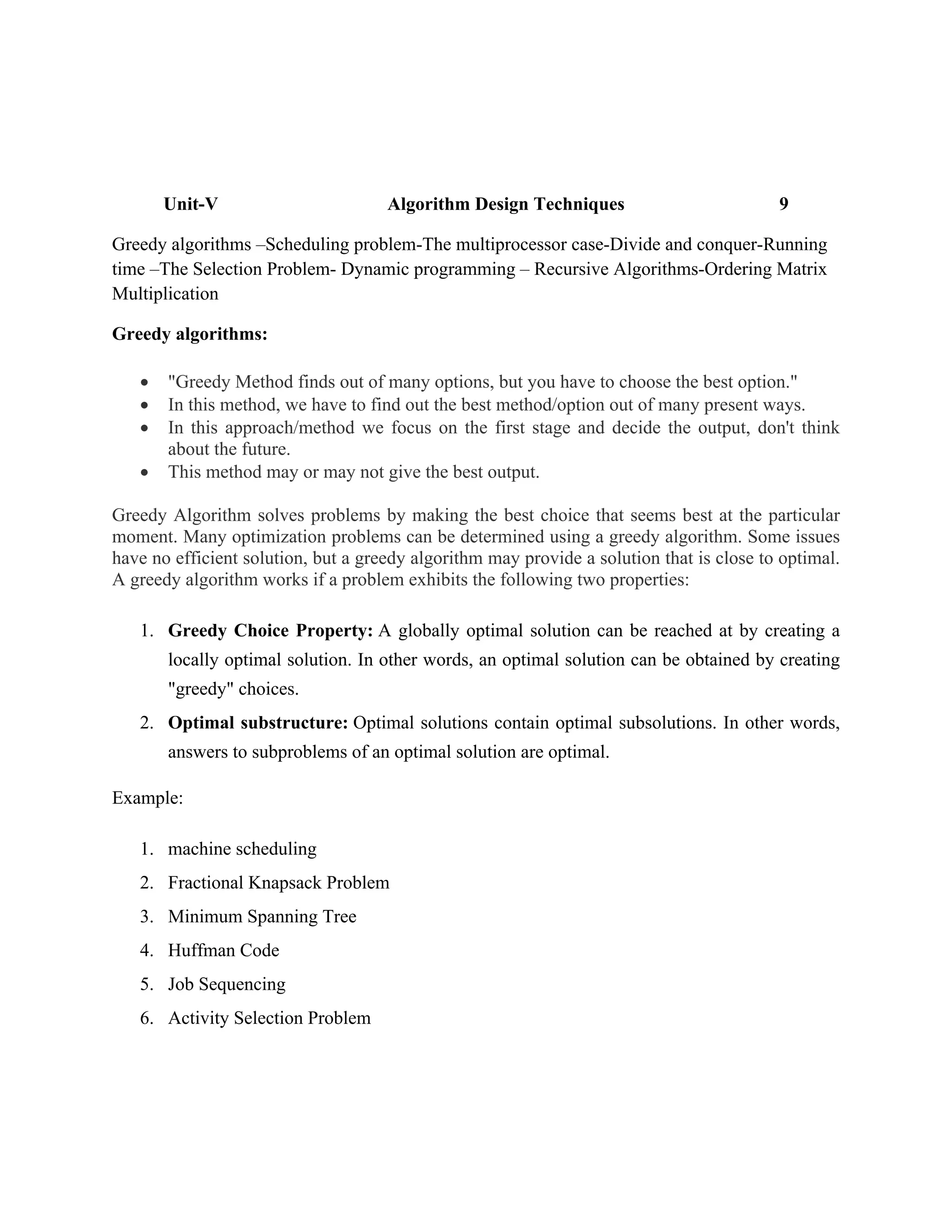
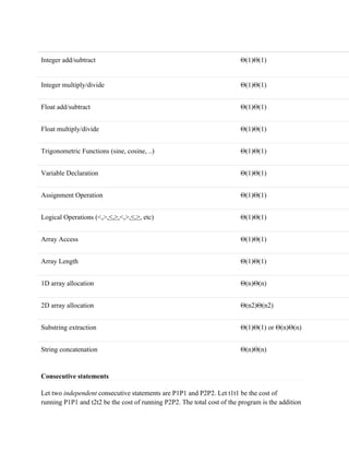
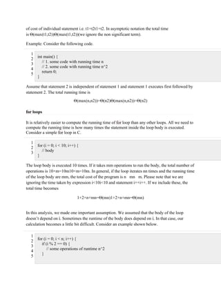
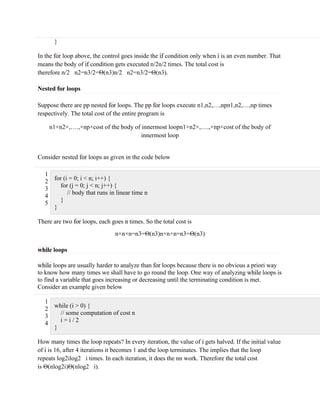
The document discusses various algorithm design techniques including greedy algorithms, divide and conquer, and dynamic programming. It provides examples of greedy algorithms like job scheduling and activity selection. It also explains the divide and conquer approach with examples like merge sort, quicksort, and closest pair of points problems. Finally, it discusses running time analysis and big-O notation for classifying algorithms based on time complexity.


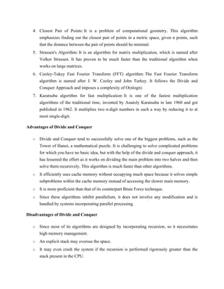
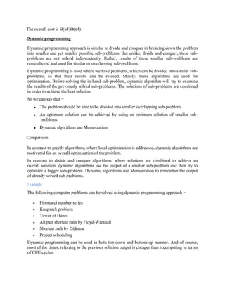
![Scheduling problem
The activity search problem is a mathematical search optimization problem. This is used in
scheduling a single resource among several ongoing and incoming processes. A greedy
algorithm provides the best solution for selecting the maximum size set of compatible activities.
Let S = {1,2,3,…n) be a set of n proposed processes. Resources can be used by only one process
at a time. Start time of activities = {s1,s2,s3,….sn} and finish time = {f1,f2,f3,…fn}. Start time
is always less than finish time.
If activity “i” starts meanwhile the half-open time interval [si, fi), then, activities i and j are said
to be compatible if the intervals (si, fi) and [si, fi) do not overlap.
Algorithm:
activity_selector (s, f)
Step 1: n ← len[s]
Step 2: A ← {1}
Step 3: j ← 1.
Step 4: for i ← 2 to n
Step 5: do if si ≥ fi
Step 6: then A ← A U {i}
Step 7: j ← i
Step 8: return A
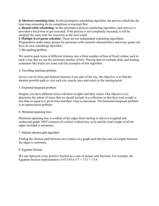
Example :
S={A1,A2,A3,A4,A5}
si={1,1,2,3,4}
fi={4,2,4,7,6}
Step 1. Arrange in increasing order of finish time.
Activity A2 A3 A1 A5 A4
si 1 2 1 4 3
fi 2 4 4 6 7
Step 2: Schedule A2](https://image.slidesharecdn.com/unitv-220703055333-68ee7da5/85/Unit-V-pdf-4-320.jpg)
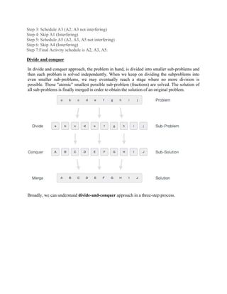
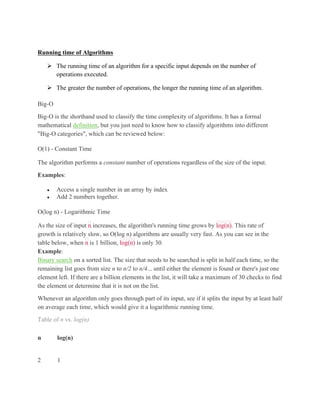

![Example 2
1
2
3
4
5
6
7
8
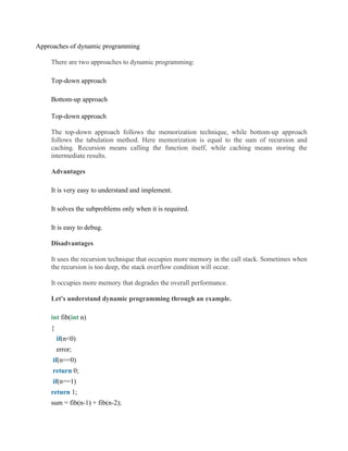
int array_sum(int a, int n) {
int i;
int sum = 0;
for (i = 0; i < n; i++) {
sum = sum + a[i]
}
return sum;
}
Analysis
1. Line 2 is a variable declaration. The cost is Θ(1)Θ(1)
2. Line 3 is a variable declaration and assignment. The cost is Θ(2)Θ(2)
3. Line 4 - 6 is a for loop that repeats nn times. The body of the for loop requires Θ(1)Θ(1) to
run. The total cost is Θ(n)Θ(n).
4. Line 7 is a return statement. The cost is Θ(1)Θ(1).
1, 2, 3, 4 are consecutive statements so the overall cost is Θ(n)Θ(n)
Example 3
1
2
3
4
5
6
7
8
9
10
11
12
int sum = 0;
for (i = 0; i < n; i++) {
for (j = 0; j < n; j++) {
for (k = 0; k < n; k++) {
if (i == j == k) {
for (l = 0; l < n*n*n; l++) {
sum = i + j + k + l;
}
}
}
}
}
Analysis
1. Line 1 is a variable declaration and initialization. The cost is Θ(1)Θ(1)
2. Line 2 - 11 is a nested for loops. There are four for loops that repeat nn times. After the
third for loop in Line 4, there is a condition of i == j == k. This condition is true
only nn times. So the total cost of these loops is Θ(n3)+Θ(n4)=Θ(n4)Θ(n3)+Θ(n4)=Θ(n4)](https://image.slidesharecdn.com/unitv-220703055333-68ee7da5/85/Unit-V-pdf-17-320.jpg)
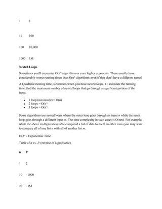
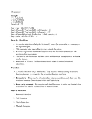
![}
In the above code, we have used the recursive approach to find out the Fibonacci series.
When the value of 'n' increases, the function calls will also increase, and computations will
also increase. In this case, the time complexity increases exponentially, and it becomes 2n
.
One solution to this problem is to use the dynamic programming approach. Rather than
generating the recursive tree again and again, we can reuse the previously calculated value. If
we use the dynamic programming approach, then the time complexity would be O(n).
When we apply the dynamic programming approach in the implementation of the Fibonacci
series, then the code would look like:
static int count = 0;
int fib(int n)
{
if(memo[n]!= NULL)
return memo[n];
count++;
if(n<0)
error;
if(n==0)
return 0;
if(n==1)
return 1;
sum = fib(n-1) + fib(n-2);
memo[n] = sum;
}
In the above code, we have used the memorization technique in which we store the results in
an array to reuse the values. This is also known as a top-down approach in which we move
from the top and break the problem into sub-problems.
Bottom-Up approach
The bottom-up approach is also one of the techniques which can be used to implement the
dynamic programming. It uses the tabulation technique to implement the dynamic
programming approach. It solves the same kind of problems but it removes the recursion. If
we remove the recursion, there is no stack overflow issue and no overhead of the recursive](https://image.slidesharecdn.com/unitv-220703055333-68ee7da5/85/Unit-V-pdf-20-320.jpg)
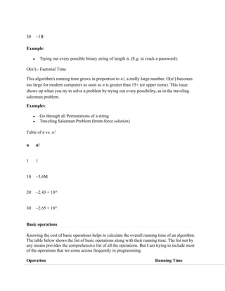
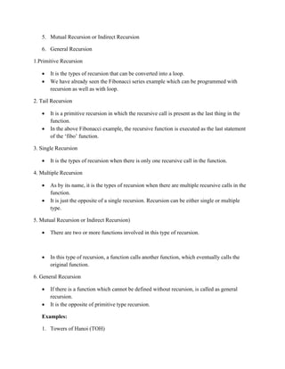
![functions. In this tabulation technique, we solve the problems and store the results in a
matrix.
There are two ways of applying dynamic programming:
Top-Down
Bottom-Up
The bottom-up is the approach used to avoid the recursion, thus saving the memory space.
The bottom-up is an algorithm that starts from the beginning, whereas the recursive
algorithm starts from the end and works backward. In the bottom-up approach, we start from
the base case to find the answer for the end. As we know, the base cases in the Fibonacci
series are 0 and 1. Since the bottom approach starts from the base cases, so we will start from
0 and 1.
Key points
We solve all the smaller sub-problems that will be needed to solve the larger sub-
problems then move to the larger problems using smaller sub-problems.
We use for loop to iterate over the sub-problems.
The bottom-up approach is also known as the tabulation or table filling method.
Example: Fractional Knapsack Problem
Optimization problem where it is possible to select fractional items rather than binary choices of
0 and 1. The binary problem cannot be solved by a greedy approach.
Step 1: Calculate the value per pound.
Step 2: Take the maximum possible amount of substance with the maximum value per pound.
Step 3: If that amount is exhausted, and we have space, take the maximum possible amount of
substance with the next maximum value per pound.
Step 4: Sort the item values per pound, greedy algorithm has a time complexity of O(n log n ).
Algorithm:
fractional knapsack (Array w, Array v, int C)
1. for i= 1 to size (v)
2. do vpp [i] = v [i] / w [i]
3. Sort-Descending (vpp)
4. i ← 1
5. while (C>0)
6. do amt = min (C, w [i])
7. sol [i] = amt
8. C= C-amt
9. i ← i+1](https://image.slidesharecdn.com/unitv-220703055333-68ee7da5/85/Unit-V-pdf-21-320.jpg)
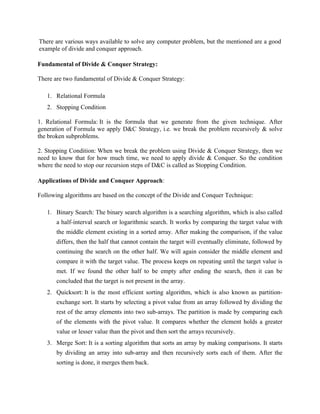
![ Matrix chain multiplication (or the matrix chain ordering problem[citation needed]) is
an optimization problem concerning the most efficient way to multiply a given sequence
of matrices.
The problem is not actually to perform the multiplications, but merely to decide the
sequence of the matrix multiplications involved.
The problem may be solved using dynamic programming.
There are many options because matrix multiplication is associative.
In other words, no matter how the product is parenthesized, the result obtained will
remain the same.
For example, for four matrices A, B, C, and D, there are five possible options:
((AB)C)D = (A(BC))D = (AB)(CD) = A((BC)D) = A(B(CD)).
Although it does not affect the product, the order in which the terms are parenthesized
affects the number of simple arithmetic operations needed to compute the product, that is,
the computational complexity.
For example, if A is a 10 × 30 matrix, B is a 30 × 5 matrix, and C is a 5 × 60 matrix, then
computing (AB)C needs (10×30×5) + (10×5×60) = 1500 + 3000 = 4500 operations,
while computing A(BC) needs (30×5×60) + (10×30×60) = 9000 + 18000 = 27000
operations.
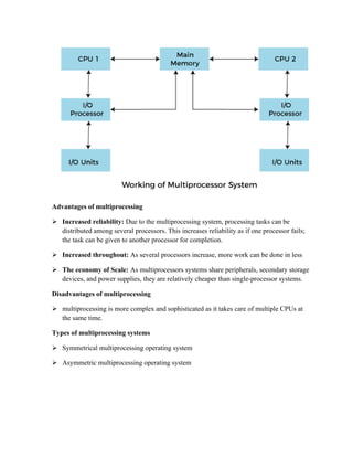
The multiprocessor case
Multiprocessing, in computing, a mode of operation in which two or more processors in a
computer simultaneously process two or more different portions of the same program (set
of instructions).
Multiprocessing is typically carried out by two or more microprocessors, each of which is
in effect a central processing unit (CPU) on a single tiny chip.
Supercomputers typically combine millions of such microprocessors to interpret and
execute instructions.](https://image.slidesharecdn.com/unitv-220703055333-68ee7da5/85/Unit-V-pdf-26-320.jpg)