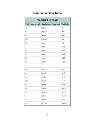
This document provides a table of standard unit conversion prefixes and multipliers as well as conversion factors between many standard units of measurement for length, volume, temperature, mass, force, energy, power, pressure, and other physical quantities. It lists the standard symbol and definition for each unit and provides the calculation to convert between related units.
English System Unit Conversion
Metric System Unit Conversion
Length Metric and English Conversion
Weight Metric and English Conversion
Volume Metric and Englis Conversion
Temperature Metric and English Conversion
Time Metric and English Conversion
Metric to Metric Equivalents
English to English Equivalents
Metric to English Equivalents
With great pleasure and enthusiasm, Thermodyne Engineering Systems present you with the maiden edition of our Thermodyne Boiler Bible. With an industrial presence of 24 years and serving a vast variety of clients the undersigned felt a special bond of respect and gratitude for all of you who made us grow with yourselves.for More Detail visit our website http://www.thermodyneboilers.com/
Cancer cell metabolism: special Reference to Lactate PathwayAADYARAJPANDEY1
Normal Cell Metabolism:
Cellular respiration describes the series of steps that cells use to break down sugar and other chemicals to get the energy we need to function.
Energy is stored in the bonds of glucose and when glucose is broken down, much of that energy is released.
Cell utilize energy in the form of ATP.
The first step of respiration is called glycolysis. In a series of steps, glycolysis breaks glucose into two smaller molecules - a chemical called pyruvate. A small amount of ATP is formed during this process.
Most healthy cells continue the breakdown in a second process, called the Kreb's cycle. The Kreb's cycle allows cells to “burn” the pyruvates made in glycolysis to get more ATP.
The last step in the breakdown of glucose is called oxidative phosphorylation (Ox-Phos).
It takes place in specialized cell structures called mitochondria. This process produces a large amount of ATP. Importantly, cells need oxygen to complete oxidative phosphorylation.
If a cell completes only glycolysis, only 2 molecules of ATP are made per glucose. However, if the cell completes the entire respiration process (glycolysis - Kreb's - oxidative phosphorylation), about 36 molecules of ATP are created, giving it much more energy to use.
IN CANCER CELL:
Unlike healthy cells that "burn" the entire molecule of sugar to capture a large amount of energy as ATP, cancer cells are wasteful.
Cancer cells only partially break down sugar molecules. They overuse the first step of respiration, glycolysis. They frequently do not complete the second step, oxidative phosphorylation.
This results in only 2 molecules of ATP per each glucose molecule instead of the 36 or so ATPs healthy cells gain. As a result, cancer cells need to use a lot more sugar molecules to get enough energy to survive.
introduction to WARBERG PHENOMENA:
WARBURG EFFECT Usually, cancer cells are highly glycolytic (glucose addiction) and take up more glucose than do normal cells from outside.
Otto Heinrich Warburg (; 8 October 1883 – 1 August 1970) In 1931 was awarded the Nobel Prize in Physiology for his "discovery of the nature and mode of action of the respiratory enzyme.
WARNBURG EFFECT : cancer cells under aerobic (well-oxygenated) conditions to metabolize glucose to lactate (aerobic glycolysis) is known as the Warburg effect. Warburg made the observation that tumor slices consume glucose and secrete lactate at a higher rate than normal tissues.
Earliest Galaxies in the JADES Origins Field: Luminosity Function and Cosmic ...Sérgio Sacani
We characterize the earliest galaxy population in the JADES Origins Field (JOF), the deepest
imaging field observed with JWST. We make use of the ancillary Hubble optical images (5 filters
spanning 0.4−0.9µm) and novel JWST images with 14 filters spanning 0.8−5µm, including 7 mediumband filters, and reaching total exposure times of up to 46 hours per filter. We combine all our data
at > 2.3µm to construct an ultradeep image, reaching as deep as ≈ 31.4 AB mag in the stack and
30.3-31.0 AB mag (5σ, r = 0.1” circular aperture) in individual filters. We measure photometric
redshifts and use robust selection criteria to identify a sample of eight galaxy candidates at redshifts
z = 11.5 − 15. These objects show compact half-light radii of R1/2 ∼ 50 − 200pc, stellar masses of
M⋆ ∼ 107−108M⊙, and star-formation rates of SFR ∼ 0.1−1 M⊙ yr−1
. Our search finds no candidates
at 15 < z < 20, placing upper limits at these redshifts. We develop a forward modeling approach to
infer the properties of the evolving luminosity function without binning in redshift or luminosity that
marginalizes over the photometric redshift uncertainty of our candidate galaxies and incorporates the
impact of non-detections. We find a z = 12 luminosity function in good agreement with prior results,
and that the luminosity function normalization and UV luminosity density decline by a factor of ∼ 2.5
from z = 12 to z = 14. We discuss the possible implications of our results in the context of theoretical
models for evolution of the dark matter halo mass function.
Introduction:
RNA interference (RNAi) or Post-Transcriptional Gene Silencing (PTGS) is an important biological process for modulating eukaryotic gene expression.
It is highly conserved process of posttranscriptional gene silencing by which double stranded RNA (dsRNA) causes sequence-specific degradation of mRNA sequences.
dsRNA-induced gene silencing (RNAi) is reported in a wide range of eukaryotes ranging from worms, insects, mammals and plants.
This process mediates resistance to both endogenous parasitic and exogenous pathogenic nucleic acids, and regulates the expression of protein-coding genes.
What are small ncRNAs?
micro RNA (miRNA)
short interfering RNA (siRNA)
Properties of small non-coding RNA:
Involved in silencing mRNA transcripts.
Called “small” because they are usually only about 21-24 nucleotides long.
Synthesized by first cutting up longer precursor sequences (like the 61nt one that Lee discovered).
Silence an mRNA by base pairing with some sequence on the mRNA.
Discovery of siRNA?
The first small RNA:
In 1993 Rosalind Lee (Victor Ambros lab) was studying a non- coding gene in C. elegans, lin-4, that was involved in silencing of another gene, lin-14, at the appropriate time in the
development of the worm C. elegans.
Two small transcripts of lin-4 (22nt and 61nt) were found to be complementary to a sequence in the 3' UTR of lin-14.
Because lin-4 encoded no protein, she deduced that it must be these transcripts that are causing the silencing by RNA-RNA interactions.
Types of RNAi ( non coding RNA)
MiRNA
Length (23-25 nt)
Trans acting
Binds with target MRNA in mismatch
Translation inhibition
Si RNA
Length 21 nt.
Cis acting
Bind with target Mrna in perfect complementary sequence
Piwi-RNA
Length ; 25 to 36 nt.
Expressed in Germ Cells
Regulates trnasposomes activity
MECHANISM OF RNAI:
First the double-stranded RNA teams up with a protein complex named Dicer, which cuts the long RNA into short pieces.
Then another protein complex called RISC (RNA-induced silencing complex) discards one of the two RNA strands.
The RISC-docked, single-stranded RNA then pairs with the homologous mRNA and destroys it.
THE RISC COMPLEX:
RISC is large(>500kD) RNA multi- protein Binding complex which triggers MRNA degradation in response to MRNA
Unwinding of double stranded Si RNA by ATP independent Helicase
Active component of RISC is Ago proteins( ENDONUCLEASE) which cleave target MRNA.
DICER: endonuclease (RNase Family III)
Argonaute: Central Component of the RNA-Induced Silencing Complex (RISC)
One strand of the dsRNA produced by Dicer is retained in the RISC complex in association with Argonaute
ARGONAUTE PROTEIN :
1.PAZ(PIWI/Argonaute/ Zwille)- Recognition of target MRNA
2.PIWI (p-element induced wimpy Testis)- breaks Phosphodiester bond of mRNA.)RNAse H activity.
MiRNA:
The Double-stranded RNAs are naturally produced in eukaryotic cells during development, and they have a key role in regulating gene expression .
Professional air quality monitoring systems provide immediate, on-site data for analysis, compliance, and decision-making.
Monitor common gases, weather parameters, particulates.
The increased availability of biomedical data, particularly in the public domain, offers the opportunity to better understand human health and to develop effective therapeutics for a wide range of unmet medical needs. However, data scientists remain stymied by the fact that data remain hard to find and to productively reuse because data and their metadata i) are wholly inaccessible, ii) are in non-standard or incompatible representations, iii) do not conform to community standards, and iv) have unclear or highly restricted terms and conditions that preclude legitimate reuse. These limitations require a rethink on data can be made machine and AI-ready - the key motivation behind the FAIR Guiding Principles. Concurrently, while recent efforts have explored the use of deep learning to fuse disparate data into predictive models for a wide range of biomedical applications, these models often fail even when the correct answer is already known, and fail to explain individual predictions in terms that data scientists can appreciate. These limitations suggest that new methods to produce practical artificial intelligence are still needed.
In this talk, I will discuss our work in (1) building an integrative knowledge infrastructure to prepare FAIR and "AI-ready" data and services along with (2) neurosymbolic AI methods to improve the quality of predictions and to generate plausible explanations. Attention is given to standards, platforms, and methods to wrangle knowledge into simple, but effective semantic and latent representations, and to make these available into standards-compliant and discoverable interfaces that can be used in model building, validation, and explanation. Our work, and those of others in the field, creates a baseline for building trustworthy and easy to deploy AI models in biomedicine.
Bio
Dr. Michel Dumontier is the Distinguished Professor of Data Science at Maastricht University, founder and executive director of the Institute of Data Science, and co-founder of the FAIR (Findable, Accessible, Interoperable and Reusable) data principles. His research explores socio-technological approaches for responsible discovery science, which includes collaborative multi-modal knowledge graphs, privacy-preserving distributed data mining, and AI methods for drug discovery and personalized medicine. His work is supported through the Dutch National Research Agenda, the Netherlands Organisation for Scientific Research, Horizon Europe, the European Open Science Cloud, the US National Institutes of Health, and a Marie-Curie Innovative Training Network. He is the editor-in-chief for the journal Data Science and is internationally recognized for his contributions in bioinformatics, biomedical informatics, and semantic technologies including ontologies and linked data.
Multi-source connectivity as the driver of solar wind variability in the heli...Sérgio Sacani
The ambient solar wind that flls the heliosphere originates from multiple
sources in the solar corona and is highly structured. It is often described
as high-speed, relatively homogeneous, plasma streams from coronal
holes and slow-speed, highly variable, streams whose source regions are
under debate. A key goal of ESA/NASA’s Solar Orbiter mission is to identify
solar wind sources and understand what drives the complexity seen in the
heliosphere. By combining magnetic feld modelling and spectroscopic
techniques with high-resolution observations and measurements, we show
that the solar wind variability detected in situ by Solar Orbiter in March
2022 is driven by spatio-temporal changes in the magnetic connectivity to
multiple sources in the solar atmosphere. The magnetic feld footpoints
connected to the spacecraft moved from the boundaries of a coronal hole
to one active region (12961) and then across to another region (12957). This
is refected in the in situ measurements, which show the transition from fast
to highly Alfvénic then to slow solar wind that is disrupted by the arrival of
a coronal mass ejection. Our results describe solar wind variability at 0.5 au
but are applicable to near-Earth observatories.
Richard's entangled aventures in wonderlandRichard Gill
Since the loophole-free Bell experiments of 2020 and the Nobel prizes in physics of 2022, critics of Bell's work have retreated to the fortress of super-determinism. Now, super-determinism is a derogatory word - it just means "determinism". Palmer, Hance and Hossenfelder argue that quantum mechanics and determinism are not incompatible, using a sophisticated mathematical construction based on a subtle thinning of allowed states and measurements in quantum mechanics, such that what is left appears to make Bell's argument fail, without altering the empirical predictions of quantum mechanics. I think however that it is a smoke screen, and the slogan "lost in math" comes to my mind. I will discuss some other recent disproofs of Bell's theorem using the language of causality based on causal graphs. Causal thinking is also central to law and justice. I will mention surprising connections to my work on serial killer nurse cases, in particular the Dutch case of Lucia de Berk and the current UK case of Lucy Letby.
2. 2
Standard Units
Unit Symbol Definition Comments
Time
second sec 1 s
minute min 60 s
hour hr 60 min
hour hour 1 hr alternate symbol
hour h 1 hr alternate symbol
day day 24 hr
shake shake 10 ns
Hertz Hz 1 s^-1
Length or Distance
international foot ft 0.3048 m
inch in 1.0/12.0 ft
international mile mile 5280.0 ft
international mile mi 1 mile alternate symbol
milli-inch mil 0.001 in
Parsec pc 3.085678e16 m
League league 3 mile
Astronomical Unit ua 1.49598e11 m
Astronomical Unit AU 1.49598e11 m alternate symbol
yard yd 3 ft
Angstrom Ang 1e-10 m
Angstrom AA 1 Ang alternate symbol
furlong furlong 220 yd
3. 3
fathom fathom 6 ft
Rod rd 16.5 ft
U.S. survey foot sft
(1200./3937.)
m
U.S. survey mile smi 5280 sft also called statue mile
point pt 1./72. in Typeface Point
pica pica 1./6. in Typeface Pica
Temperature
Celsius C 1 K -273.15
Rankine R 5.0/9.0 K
Fahrenheit F 1 R -459.67
Mass
gram g 0.001 kg This is case sensitive.
gram gm g (alternate symbol)
pound mass lbm 0.45359237 kg (avoirdupois)
Troy pound lbt 0.3732417 kg (apothecary)
carat (metric) carat 0.2 g
slug slug 1 lb sec^2/ft
snail snail 1 lb sec^2/in
Short Ton ton 2000 lbm
Long Ton ton_l 2240 lbm
Ounce oz 28.34952 g (avoirdupois)
Grain gr 64.79891 mg
Pennyweight dwt 1.55174 g
Force or Weight
Newton N 1 kg m/s^2
4. 4
Dyne dyn 1e-5 N
pound force lb lbm G
pound force lbf lbm G
poundal poundal 1 lbm ft/sec^2
kilopound kip 1000 lbf
kilogram force kgf kg G
Energy
Joule J 1 N m
British Therm.
Unit
BTU 1055.056 J (International Table)
British Therm.
Unit
Btu 1 BTU alternate symbol
British Therm.
Unit
BTU_th 1054.350 J (Thermochemical)
calorie cal 4.1868 J (International Table)
calorie cal_th 4.184 J (Thermochemical)
Calorie Cal 4.1868 kJ (nutritionists)
electron volt eV 1.602177e-19 J
erg erg 1e-7 J
Ton of TNT TNT 4.184e9 J
Power
Watt W 1 J/s
Horse Power hp 550 ft lb/s
Pressure
bar bar 1e5 N/m^2
Pascal Pa 1 N/m^2
Pounds per sq. inch psi 1 lb/in^2
5. 5
Pounds per sq. ft. psf 1 lb/ft^2
kilo psi ksi 1000.0 psi
atmospheres atm
1.01325e5
N/m^2
inches of Mercury inHg 3.387 kPa
millimeters
Mercury
mmHg 0.1333 kPa
Torr torr 1.333224 Pa
Volume or Area
Liter L 1/1000.0 m^3
gallon gal 3.785412 L
Pint (U.S. liquid) pint 1/8. gal
Quart (U.S. liquid) qt 2 pint
Pint (U.S. dry) dpint 0.5506105 L
Quart (U.S. dry) dqt 2 dpint
Acre acre 1/640.0 smi^2
Hectare ha 10000 m^2
Barrel (petroleum) barrel 158.9873 L
Fluid Ounce oz_fl 29.57353 mL
Gill (U.S.) gi 0.1182941 L
Peck (U.S.) pk 8.809768 L
Tablespoon tbl 1/32. pint
Teaspoon tsp 1/3. tbl
Cup cup 16. tbl
Electromagnetism
Coulomb Co 1 A s Electric Charge
Volt V 1 W/A Electric Potential
6. 6
Ohm ohm 1 V/A Electric Resistance
Ohm Omega 1 V/A alternate symbol
Faraday faraday 96485.31 Co Electric Charge
Farad farad Co/V Capacitance
Stokes stokes 1e-4 m^2/s
Oersted Oe 79.57747 A/m
Webber Wb V s Magnetic flux
Tesla Tesla Wb/m^2 Magnetic flux density
Henry H Wb/A Inductance
Siemens S A/V Electrical Conductance
Light and Radiation
Lux lux cd/m^2 Iluminance
Lux lx cd/m^2
Lumen lm cd Luminous Flux
Stilb sb 10000 cd/m^2
Phot ph 10000 lx
Becquerel Bq s^-1 activity
Gray Gy J/kg Absorbed Dose, kerma
Sievert Sv J/kg Dose equivalent
Other Quantities
pound mole lbmole 1 mol lbm/g quantity
poise poise 1 g /sec cm viscosity
Gravity's accel. G
9.80665
m/sec^2
Gravity on Earth
Degree deg Pi/180
Can be used to convert from degrees to
radians for trig functions.
Percent % 0.01
7. 7
Knot knot 1852 m/hr velocity
Miles per Hour mph 1 mi/hr velocity
Gallon/minute gpm 1. gal/min flow rate
Revolution/minute rpm 360 deg/min
TO CONVERT FROM DO THIS
Atmospheres to inches of mercury @32°F
(Atm to inHg32)
(atm) * 29.9213 = (inHg32)
Atmospheres to inches of mercury @60°F
(Atm to inHg60)
(atm) * 30.0058 = (inHg60)
Atmospheres to millibars (atm to mb) (atm) * 1013.25 = (mb)
Atmospheres to pascals (atm to Pa) (atm) * 101325 = (Pa)
Atmospheres to pounds/square inch (atm to lb/in^2) (atm) * 14.696 = (lb/in^2)
Centimeters to feet (cm to ft) (cm) * 0.032808399 = (ft)
Centimeters to inches (cm to in) (cm) * 0.39370079 = (in)
Centimeters to meters (cm to m) (cm) * 0.01 = (m)
Centimeters to millimeters (cm to mm) (cm) * 10 = (mm)
Degrees to radians (deg to rad) (deg) * 0.01745329 = (rad)
Degrees Celsius to degrees Fahrenheit (C to F) [(C) * 1.8] + 32 = (F)
Degrees Celsius to degrees Kelvin (C to K) (C) + 273.15 = (K)
Degrees Celsius to degrees Rankine (C to R) [(C) * 1.8] + 491.67 = (R)
Degrees Fahrenheit to degrees Celsius (F to C) [(F) - 32)] * 0.555556 = (C)
Degrees Fahrenheit to degrees Kelvin (F to K) [(F) * 0.555556] + 255.37 = (K)
Degrees Fahrenheit to degrees Rankine (F to R) (F) + 459.67 = (R)
Degrees Kelvin to degrees Celsius (K to C) (K) - 273.15 = (C)
Degrees Kelvin to degrees Fahrenheit (K to F) [(K) - 255.37] * 1.8 = (F)
8. 8
Degrees Kelvin to degrees Rankine (K to R) (K) * 1.8 = (R)
Degrees Rankine to degrees Celsius (R to C) [(R) - 491.67] * 0.555556 = (C)
Degrees Rankine to degrees Fahrenheit (R to F) (R) - 459.67 = (F)
Degrees Rankine to degrees Kelvin (R to K) (R) * 0.555556 = (K)
Feet to Centimeters (ft to cm) (ft) * 30.48 = (cm)
Feet to meters (ft to m) (ft) * 0.3048 = (ft to m)
Feet to miles (ft to mi) (ft) * 0.000189393 = (mi)
Feet/minute to meters/second
(ft/min to m/s)
(ft/min) * 0.00508 = (m/s)
Feet/minute to miles/hour (ft/min to mph) (ft/min) * 0.01136363 = (mph)
Feet/second to kilometers/hour (ft/s to kph) (ft/s) * 1.09728 = (kph)
Feet/second to knots (ft/s to kt) (ft/s) * 0.5924838 = (kt)
Feet/second to meters/second (ft/s to m/s) (ft/s) * 0.3048 = (m/s)
Feet/second to miles/hour (ft/s to mph) (ft/s) * 0.681818 = (mph)
Grams/cubic centimeter to pounds/cubic foot
(gm/cm^3 to lb/ft^3)
(gm/cm^3) * 62.427961 = (lb/ft^3)
Grams/cubic meter to pounds/cubic foot
(gm/m^3 to lb/ft^3)
(gm/m^3) * 0.000062427961 =
(lb/ft^3)
Hectopascals to millibars (hPa to mb) Nothing - they are equivalent units
Inches to centimeters (in to cm) (in) * 2.54 = (cm)
Inches to millimeters (in to mm) (in) * 25.4 = (mm)
Inches of mercury @32°F to atmospheres
(inHg32 to atm)
(inHg32) * 0.0334211 = (atm)
Inches of mercury @32°F to millibars (inHg32 to mb) (inHg32) * 33.8639 = (mb)
Inches of mercury @32°F to pounds/square inch
(inHg32 to lb/in^2)
(inHg32) * 0.49115 = (lb/in^2)
Inches of mercury @60°F to atmospheres
(inHg60 to atm)
(inHg60) * 0.0333269 = (atm)
9. 9
Inches of mercury @60°F to millibars (inHg60 to mb) (inHg60) * 33.7685 = (mb)
Inches of mercury @60°F to pounds/square inch
(inHg60 to lb/in^2)
(inHg60) * 0.48977 = (lb/in^2)
Kilograms/cubic meters to pounds/cubic foot
(kg/m^3 to lb/ft^3)
(kg/m^3) * 0.062427961 = (lb/ft^3)
Kilograms/cubic meters to slugs/cubic foot
(kg/m^3 to slug/ft^3)
(kg/m^3) * 0.001940323 =
(slug/ft^3)
Kilometers to meters (km to m) (km) * 1000 = (m)
Kilometers to miles (km to mi) (km) * 0.62137119 = (mi)
Kilometers to nautical miles (km to nmi) (km) * 0.5399568 = (nmi)
Kilometers/hour to feet/second (kph to ft/s) (kph) * 0.91134 = (ft/s)
Kilometers/hour to knots (kph to kt) (kph) * 0.5399568 = (kt)
Kilometers/hour to meters/second (kph to m/s) (kph) * 0.277777 = (m/s)
Kilometers/hour to miles/hour (kph to mph) (kph) * 0.62137119 = (mph)
Kilopascals to millibars (kPa to mb) (kPa) * 10 = (mb)
Knots to feet/second (kt to ft/s) (kt) * 1.6878099 = (ft/s)
Knots to kilometers/hour (kt to kph) (kt) * 1.852 = (kph)
Knots to meters/second (kt to m/s) (kt) * 0.514444 = (m/s)
Knots to miles/hour (kt to mph) (kt) * 1.1507794 = (mph)
Knots to nautical miles/hour (kt to nmph) Nothing - they are equivalent units
Langleys/minute to watts/square meter
(ly/min to W/m^2)
(ly/min) * 698.339 = (W/m^2)
Watts/square meter to langleys/minute
(W/m^2 to ly/min)
(W/m^2) * 0.00143197 = (ly/min)
Meters to centimeters (m to cm) (m) * 100 = (cm)
Meters to feet (m to ft) (m) * 3.2808399 = (ft)
Meters to kilometers (m to km) (m) * 0.001 = (km)
10. 10
Meters to miles (m to mi) (m) * 0.00062137119 = (mi)
Meters/second to feet/minute (m/s to ft/min) (m/s) * 196.85039 = (ft/min)
Meters/second to feet/second (m/s to ft/s) (m/s) * 3.2808399 = (ft/s)
Meters/second to kilometers/hour (m/s to kph) (m/s) * 3.6 = (kph)
Meters/second to knots (m/s to kt) (m/s) * 1.943846 = (kt)
Meters/second to miles/hour (m/s to mph) (m/s) * 2.2369363 = (mph)
Miles to feet (mi to ft) (mi) * 5280 = (ft)
Miles to kilometers (mi to km) (mi) * 1.609344 = (km)
Miles to meters (mi to m) (mi) * 1609.344 = (m)
Miles/hour to feet/minute (mph to ft/min) (mph) * 88 = (ft/min)
Miles/hour to feet/second (mph to ft/s) (mph) * 1.466666 = (ft/s)
Miles/hour to kilometers/hour (mph to kph) (mph) * 1.609344 = (kph)
Miles/hour to knots (mph to kt) (mph) * 0.86897624 = (kt)
Miles/hour to meters/second (mph to m/s) (mph) * 0.44704 = (m/s)
Millibars to atmospheres (mb to atm) (mb) * 0.000986923 = (atm)
Millibars to hectopascals (mb to hPa) Nothing - they are equivalent units
Millibars to inches of mercury @32°F (mb to
inHg32)
(mb) * 0.02953 = (inHg32)
Millibars to inches of mercury @60°F (mb to
inHg60)
(mb) * 0.02961 = (inHg60)
Millibars to kilopascals (mb to kPa) (mb) * 0.1 = (kPa)
Millibars to millimeters of mercury @32°F (mb to
mmHg)
(mb) * 0.75006 = (mmHg)
Millibars to millimeters of mercury @60°F (mb to
mmHg)
(mb) * 0.75218 = (mmHg)
Millibars to newtons/square meter (mb to N/m^2) (mb) * 100 = (N/m^2)
Millibars to pascals (mb to Pa) (mb) * 100 = (Pa)
Millibars to pounds/square foot (mb to lb/ft^2) (mb) * 2.088543 = (lb/ft^2)
11. 11
Millibars to pounds/square inch (mb to lb/in^2) (mb) * 0.0145038 = (lb/in^2)
Millimeters to centimeters (mm to cm) (mm) * 0.1 = (cm)
Millimeters to inches (mm to in) (mm) * 0.039370078 = (in)
Millimeters of mercury @32°F to millibars (mmHg to
mb)
(mmHg) * 1.33322 = (mb)
Millimeters of mercury @60°F to millibars (mmHg to
mb)
(mmHg) * 1.32947 = (mb)
Nautical miles to kilometers (nmi to km) (nmi) * 1.852 = (km)
Nautical miles to statute miles (nmi to mi) (nmi) * 1.1507794 = (mi)
Nautical miles/hour to knots (nmph to kt) Nothing - they are equivalent units
Newtons/square meter to millibars (N/m^2 to mb) (N/m^2) * 0.01 = (mb)
Pascals to atmospheres (Pa to atm) (Pa) * 0.000009869 = (atm)
Pascals to millibars (Pa to mb) (Pa) * 0.01 = (mb)
Pounds/cubic foot to grams/cubic centimeter
(lb/ft^3 to gm/cm^3)
(lb/ft^3) * 0.016018463 = (gm/cm^3)
Pounds/cubic foot to grams/cubic meter
(lb/ft^3 to gm/m^3)
(lb/ft^3) * 16018.46327 = (gm/m^3)
Pounds/cubic foot to kilograms/cubic meter
(lb/ft^3 to kg/m^3)
(lb/ft^3) * 16.018463 = (kg/m^3)
Pounds/square foot to millibars (lb/ft^2 to mb) (lb/ft^2) * 0.478803 = (mb)
Pounds/square inch to atmospheres (lb/in^2 to atm) (lb/in^2) * 0.068046 = (atm)
Pounds/square inch to inches of mercury @32°F
(lb/in^2 to inHg32)
(lb/in^2) * 2.03602 = (inHg32)
Pounds/square inch to inches of mercury @60°F
(lb/in^2 to inHg60)
(lb/in^2) * 2.04177 = (inHg60)
Pounds/square inch to millibars (lb/in^2 to mb) (lb/in^2) * 68.9474483 = (mb)
Radians to degrees (rad to deg) (rad) * 57.29577951 = (deg)
Slugs/cubic foot to kilograms/cubic meter
(slug/ft^3 to kg/m^3)
(slug/ft^3) * 515.378 = (kg/m^3)