Undergraduate Mathematics For The Life Sciences Models Processes And Directions Glenn Ledder Timothy D Comar Jenna P Carpenter
Undergraduate Mathematics For The Life Sciences Models Processes And Directions Glenn Ledder Timothy D Comar Jenna P Carpenter
Undergraduate Mathematics For The Life Sciences Models Processes And Directions Glenn Ledder Timothy D Comar Jenna P Carpenter


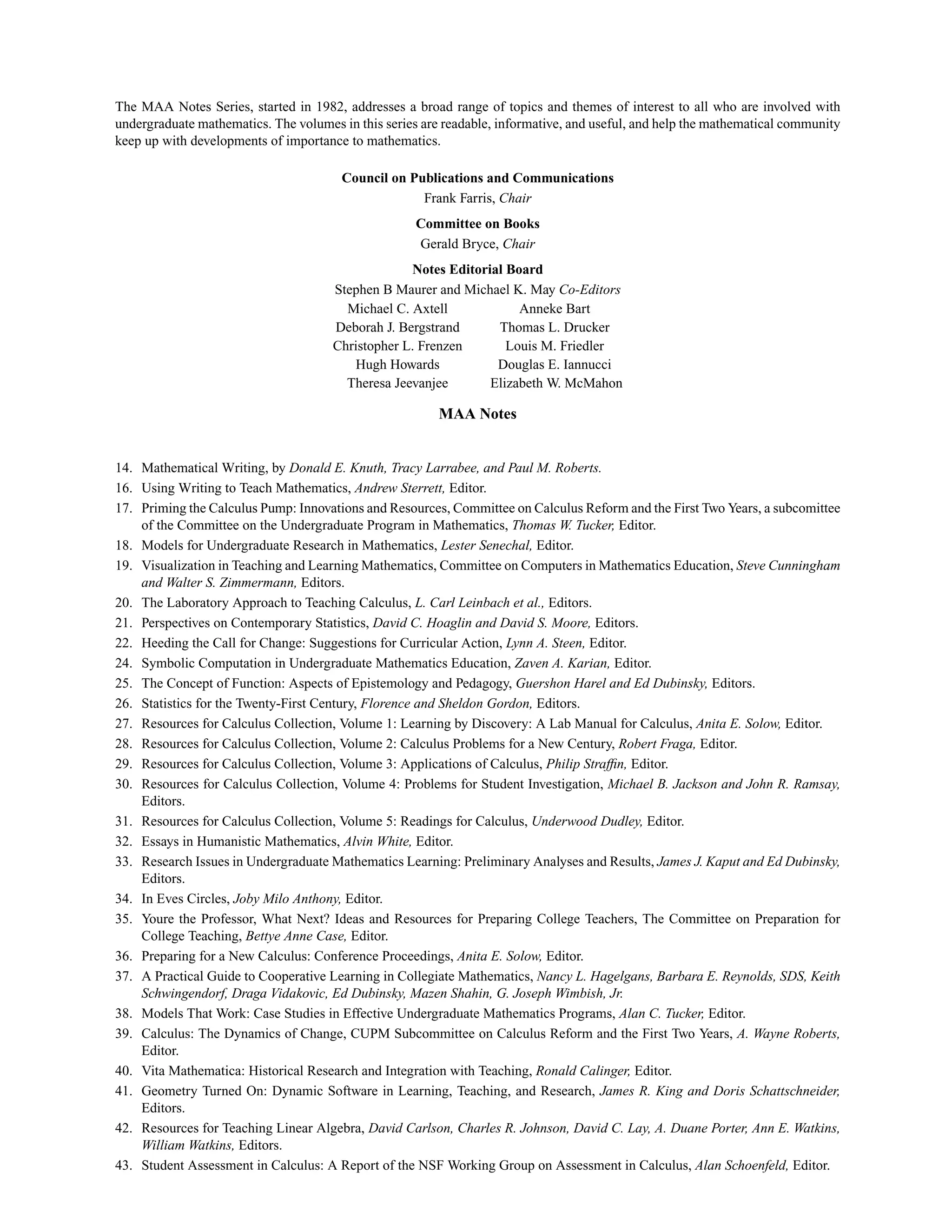


![6 Chapter 1 BioCalc at Illinois
r Average class size: Sections are capped at 20.
r Enrollment requirements: First-year students in the biological sciences. Students cannot enroll unless they are
life science majors.
r Faculty/dept per class, TAs: Typically taught by a graduate TA in mathematics or sometimes a faculty member.
There is also one undergraduate class assistant.
r Next course: Life science majors must take two of Calculus I, Calculus II, and Statistics, so some continue on to
Calculus II.
r Website: http://www-cm.math.uiuc.edu/
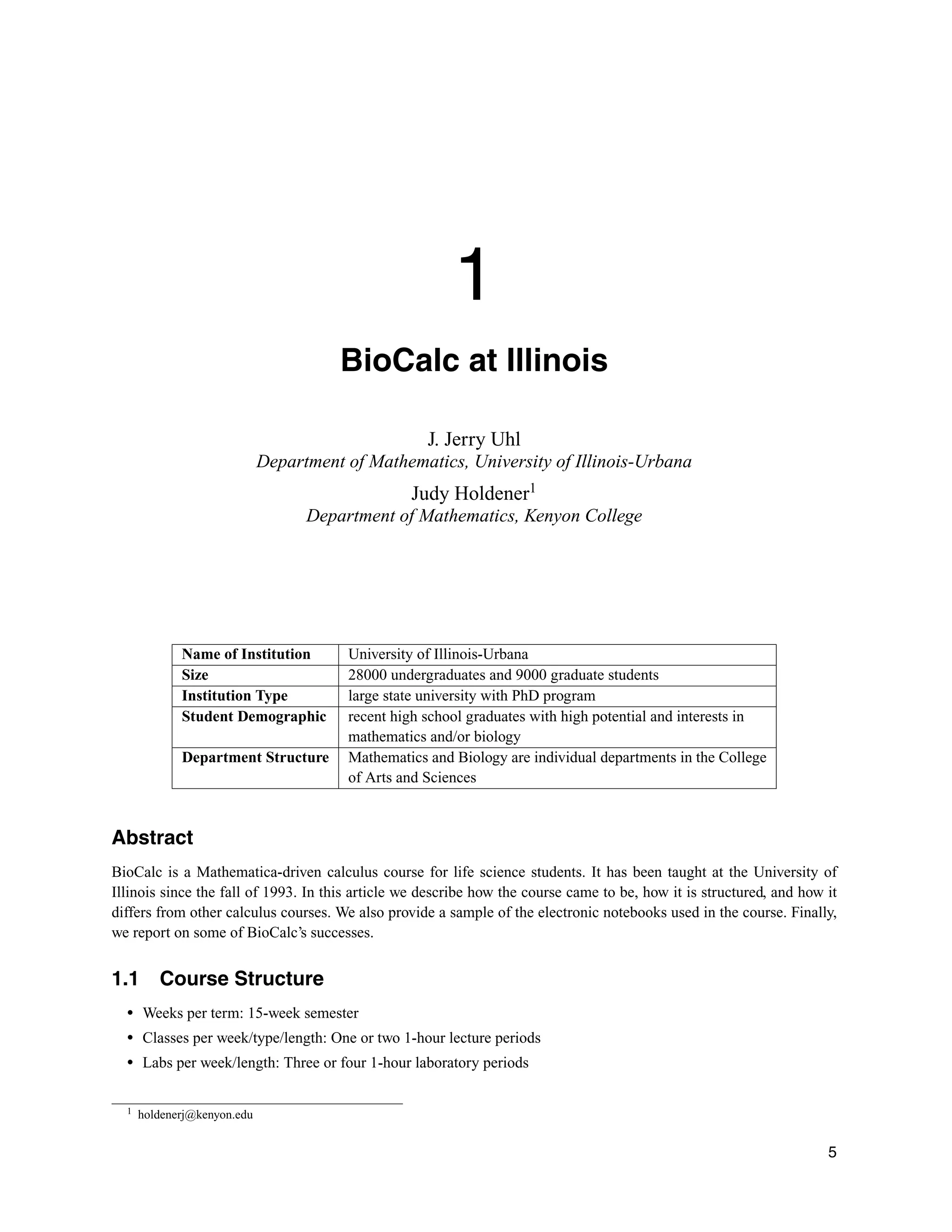
1.2 Introduction
In the late 1980s at Illinois, our Illinois-Ohio State group developed a Mathematica-based calculus course now offered
at Illinois. By the early 1990s, the Mathematica-based calculus sequence Calculus Mathematica (CM) (Uhl et al.,
2006) had been class-tested and revised. In this revision, we decided to place heavy emphasis on life science models
because our vision of calculus had become that it is the study and measurement of growth. This led the way to an
emphasis on teaching calculus with life science models. After all, what grows? Animals, populations, and epidemics
do. As our course evolved, we could see that many students from a variety of fields, including engineering, identified
better with the life science models than they did with the physics examples that are typically used in a calculus course.
At that point a fortuitous event occurred . . .
Professor Sandra Lazarowitz of the School of Life Sciences at Illinois called one of us and said that the standard
calculus course was not connecting with the life science students, who were not interested in computing the work
done by a force or the position of a projectile. The engineering emphasis in calculus sent the signal that it had little to
do with their future careers in the biological sciences. As evidence of the disconnect, Professor Lazarowitz said that
approximately 60% of the life science majors enrolled in the traditional Calculus I course were receiving a grade of C
or lower in the course. It is a common misconception that life science students are weak in mathematics. We told her
we were working on a calculus course that might be better suited for her life science students.
In the fall of 1993, two Calculus Mathematica sections were reserved for life science students. The pilot sections
were small (approximately 16 students each) and were taught by graduate teaching assistants Judy Holdener and Bill
Hammock in a computer lab located within the Life Sciences building.2
The ACT scores of the students suggested
that they would be at risk in traditional calculus, and many of the students had a high degree of math phobia. Despite
these disadvantages, the students flourished in the experimental CM sections. Professor Lazarowitz, who was also
the Director of the Howard Hughes Program for Undergraduate Education in the Life Sciences at Illinois, happily
reported “first year life science students [in Calculus Mathematica sections] are studying mathematical models
normally reserved for senior math majors, and student responses have been enthusiastic.” She was encouraged by the
success rate, reporting that life science students who would likely have dropped a traditional offering of calculus were
able to earn As with the new approach. As a result of the success of the pilot sections, the Department of Mathematics
and the School of Life Sciences entered into an agreement to call the course “BioCalc” and to make it a permanent
offering for life science students.
After seventeen years, life science students continue to flourish in BioCalc. Using university records, staff at the
Howard Hughes Medical Institute assessed the course in April of 2001 and cited the following conclusions in their
report on the course (Fahrbach et al., 2001):
r The BioCalc course is equally attractive to life sciences students required to take Math 120 (the standard calculus
course at Illinois). No life sciences option is over- or underrepresented.
r BioCalc students are as well prepared for Math 130 (the second calculus course in the standardsequence) as
non-BioCalc students, as judged by the grade obtained in Math 130.
2 This lab was funded by the Howard Hughes Medical Institute (HHMI).](https://image.slidesharecdn.com/21242735-250520085102-8b24d4e6/75/Undergraduate-Mathematics-For-The-Life-Sciences-Models-Processes-And-Directions-Glenn-Ledder-Timothy-D-Comar-Jenna-P-Carpenter-29-2048.jpg)
![8 Chapter 1 BioCalc at Illinois
1.4 The Format of BioCalc
So how are the BioCalc lessons structured and what exactly do students do in and out of class? The “textbook” is
electronic, consisting of a series of interactive Mathematica notebooks, and students learn calculus by working through
tutorial problems, experimenting with built-in Mathematica routines, and explaining graphical and computational
output. Each lesson follows the same format, with four components:
r The Basics section introduces the fundamental ideas in the lesson by presenting problems and explanations, often
visual in nature. Students are encouraged to experiment with the problems by changing functions and numbers
and rerunning the Mathematica code. Many of the problems prompt students to make conjectures about the
patterns they observe in the computer output.
r The Tutorial section, like the Basics section, presents problems for the student, but the focus is on techniques and
applications that relate to the ideas presented in the Basics section.
r The Give it a Try section is the heart of the course, providing a list of problems to be solved and submitted
(electronically) by the student. Like the Tutorial section, problems are often application-based, incorporating
models from the life sciences. Information needed to solve the problems is found in the Basics and Tutorial
sections.
r The Literacy Sheets present problems to be worked out with paper and pencil. This section is completed after the
student has already completed the electronic portions of the lesson.
Although the format may vary with the instructor, most BioCalc lessons are conducted in a computer lab. On a
typical lab day, students work through the electronic notebooks at their own pace, asking questions of the instructor
as needed. On every third or fourth session, the class meets in a standard classroom for a traditional chalkboard
discussion. Students are graded on the electronic work they complete (in the Give it a Try section of the lesson) and
the written work they do on the Literacy Sheets. Exams generally have both a written component and a computer
component.
1.5 BioCalc Sampler
In this final section, we reveal the flavor of BioCalc’s electronic lessons by examining BioCalc’s coverage of the chain
rule. The chain rule is often associated with hand computation in calculus, but BioCalc students learn it in parallel with
constructing height and weight functions to model the growth of animals over time. We will illustrate below, starting
with the first mention of the chain rule. (Incidentally, BioCalc does not allow students to rely on the computer for the
computation of derivatives, among other things. A basic literacy is expected of the students.)
In introducing the chain rule, the Basics section starts by encouraging students to look for patterns in the derivatives
of compositions of functions. What follows is taken directly from the electronic notebook covering the differentiation
rules. Mathematica syntax is in bold (the code has not been executed).
- - - -
B.2) The chain rule: D[f[g[x]],x]=(f
)[g[x]] (g
)[x]
Let’s check out the derivative of the composition of two functions.
Here is the derivative of Sin[xˆ2]:
Clear[f,x];
f[x ]=Sin[xˆ2]; (f
)[x]
Or
D[Sin[xˆ2], x]
This catches your eye because the derivative of Sin[x] is Cos[x] and the derivative of xˆ2 is 2x. It seems that the
derivative of Sin[xˆ2] is manufactured from the derivative of Sin[x] and the derivative of xˆ2. Here is the derivative
of (xˆ2+ Sin[x])ˆ8:](https://image.slidesharecdn.com/21242735-250520085102-8b24d4e6/75/Undergraduate-Mathematics-For-The-Life-Sciences-Models-Processes-And-Directions-Glenn-Ledder-Timothy-D-Comar-Jenna-P-Carpenter-31-2048.jpg)
![1.5 BioCalc Sampler 9
D[(xˆ2+Sin[x])ˆ8, x]
This catches your eye because the derivative of xˆ8 is 8 xˆ7 and the derivative of xˆ2+Sin[x] is 2x+Cos[x]. It seems
that the derivative of (xˆ2+ Sin[x])ˆ8 is manufactured from the derivative of xˆ8, the derivative of Sin[x], and the
derivative of xˆ2. Here is the derivative of f[g[x]]:
Clear[f,g]; D[f[g[x]],x]
Very interesting and of undeniable importance. This formula, which says that the derivative of h[x]=f[g[x]] is
h
[x]=f
[g[x]] g
[x], is called the chain rule. Do a check:
Clear[f,g,x];
D[f[g[x]], x]==f
[g[x]]g
[x]
The chain rule tells you how to build the derivative of f[g[x]] from the derivatives of f[x] and g[x]. Here is the chain
rule in action:
If h[x]=Sin[xˆ2], then h
[x]=Cos[xˆ2] 2 x in accordance with:
D[Sin[xˆ2], x]
And if h[x]=(xˆ2+ Sin[x])ˆ8, then h
[x]=(8 (xˆ2+ Sin[x]))ˆ7 (2 x+ Cos[x]) in accordance with:
D[(xˆ2+Sin[x])ˆ8, x]
B.2.a) Give an explanation of why the derivative of f[g[x]] is f
[g[x]] g
[x].
Answer: Put h[x]=f[g[x]].
Recall that h[x] grows h
[x] times as fast as x.
But
f[g[x]] grows f
[g[x]] times as fast as g[x]
g[x] grows g
[x] times as fast as x.
As a result, f[g[x]] grows f
[g[x]] g
[x] times as fast as x.
This explains why the instantaneous growth rate of f[g[x]] is f
[g[x]] g
[x].
In other words, the derivative of f[g[x]] with respect to x is f
[g[x]] g
[x].
This rule is called the chain rule, and it is important.
- - - -
After presenting this explanation of the chain rule, the Basics section continues with more examples, presenting the
derivatives of sin(5x), sin(x4
), (g(x))3
, f (x3
y2
) (with respect to y), and (ex
–x2
)7
.
Later in the Tutorial section, the students examine the effects of scaling on surface area and volume and use the
chain rule to explain why the instantaneous percentage growth rate of the weight of a Bernese Mountain Dog is three
times the instantaneous percentage growth rate of the height. In the excerpt of the electronic textbook that follows, the
only Mathematica output included are the plots. The rest of the output is excluded for the sake of space.
- - - -
T.3) Linear dimension: length, area, volume and weight
The volume measurement, V[r], and the surface area measurement, S[r], of a sphere of radius r are given by
V[r]=(4 [Pi] rˆ3)/3
S[r]=4 [Pi] rˆ2.
This says that V[r] is proportional to rˆ3 and S[r] is proportional to rˆ2.
For other three-dimensional objects, the formulas for volume and surface area are not so easy to come by, but the
idea of proportionality survives. Here is the idea: A linear dimension of a given solid or shape is any length between
specified locations on the solid. The radius of a sphere or the radius of a circle is a linear dimension. The total length
of a solid, the total width, and the total height of a solid are examples of linear dimensions. The diameter of the
finger loop on a coffee cup is a linear dimension of the cup.](https://image.slidesharecdn.com/21242735-250520085102-8b24d4e6/75/Undergraduate-Mathematics-For-The-Life-Sciences-Models-Processes-And-Directions-Glenn-Ledder-Timothy-D-Comar-Jenna-P-Carpenter-32-2048.jpg)
![10 Chapter 1 BioCalc at Illinois
Next take a given shape for a solid. If it stays the same but the linear dimensions change, then it is still true that the
volume is proportional to the cube of any linear dimension and it is still true that the surface area is proportional to
the square of any linear dimension.
Here is a shape in the x-y plane and the same shape with its linear dimensions increased by a factor of 3:
T.3.a) How does the area measurement of the larger blob above compare to the area measurement of the smaller
blob?
Answer: Both are the same shape, but the linear dimensions of the larger blob are three times the linear dimensions
of the smaller blob. The upshot: The area measurement of the larger blob is 3ˆ2=9 times the area of the smaller
blob.
T.3.b) The idea of linear dimension leads to some intriguing biological implications. A giant mouse with linear
dimension ten times larger than the usual mouse would not be viable because the volume of its body would be
larger than the volume of the usual mouse by a factor of 10ˆ3, but the surface area of some of its critical supporting
organs like lungs, intestines and skin would be larger only by a factor of 10ˆ2. That big mouse would be hungry and
out of breath at all times! Similarly, there will never be a 12-foot-tall basketball player at Indiana or even at Duke.
The approximate size of an adult mammal is dictated by its shape! The same common sense applies to buildings
and other structures. An architect or engineer does not design a 200-foot-tall building by taking a design for a
20-foot-tall building and multiplying all the linear dimensions by 10. Now it’s time for a calculation.
A crystal grows in such a way that all the linear dimensions increase by 25%. How do the new surface area and new
volume compare to the old surface area and volume?
Answer:
Clear[newsurfacearea,oldsurfacearea];
newsurfacearea = 1.25ˆ2 oldsurfacearea
An increase of the linear dimensions by 25% increases the surface area by about 56%.
The percentage increase in volume is:
Clear[newvolume,oldvolume];
newvolume = 1.25ˆ3 oldvolume
An increase of the linear dimensions by 25% increases the volume by about 95%.
T.3.c.i) Calculus Mathematica thanks Ruth Reynolds, owner of Pioneer Bernese Mountain Dog Kennel in
Greenwood, Florida, for the data used in this problem.
Dogs and other animals grow so that a linear dimension of their bodies is given by what a lot of folks call a logistic
function (b c eˆ(a t))/(b - c + c eˆ(a t)) , where t measures time in years elapsed since the birth of the animal. A good
linear dimension for a dog is the height of the dog’s body at the dog’s shoulders:
Clear[height,a,b,c,t];
height[t ]=(b c Eˆ(a t))/(b-c+c Eˆ(a t))](https://image.slidesharecdn.com/21242735-250520085102-8b24d4e6/75/Undergraduate-Mathematics-For-The-Life-Sciences-Models-Processes-And-Directions-Glenn-Ledder-Timothy-D-Comar-Jenna-P-Carpenter-33-2048.jpg)
![1.5 BioCalc Sampler 11
To see what the parameters a, b, and c mean, look at:
height[0]
This tells you that c measures the dog’s height at birth. The global scale of height[t]=(b c eˆ(a t))/(b - c +c eˆ(a t)) is
(b c eˆ(a t) eˆ(a t))/c=b. This tells you that b measures the dog’s mature height. For a typically magnificent Bernese
Mountain Dog, as owned by the actor Robert Redford, b=24 inches and c=4.5 inches; so for the Bernese Mountain
Dog, height[t] is:
b=24.0;
c=4.5;
height[t]
The parameter a is related to how fast the dog grows. At one year, a typical Bernese Mountain Dog has achieved
about 95% of its mature height. This gives you an equation to solve to get a:
equation=height[1]==0.95 (24.0)
Solve[equation,a]
Now you’ve got the height function for the typical Bernese Mountain Dog:
a=4.41078;
height[t]
Here’s a plot:
heightplot = Plot[{height[t],b,c},{t,0,2},PlotStyle-
{{Thickness[0.01]},{Brown},{Brown}},PlotRange-All,AxesLabel-
{t,height[t]}]
Looks OK.
Given that the typical mature Bernese Mountain Dog as described above weighs 85 pounds, give an approximate
plot of the dog’s weight as a function of time for the first three years and give a critique of the plot.
Answer: If you assume the dog maintains the same shape throughout the growing process, then you can say:
weight[t] is proportional to the volume of the dog’s body at time t and
the volume of the dog’s body at time t is proportional to height[t]ˆ3. So
weight[t] =k (height[t])ˆ3 =k ((b c eˆ(a t))/(b - c + c eˆ(a t)))ˆ3.
The global scale of weight[t] is k ((b c eˆ(a t))/(c eˆ(a t)))ˆ3=k bˆ3. For the typical Bernese Mountain Dog under
study here, k is given by:
Solve[85==bˆ3 k,k]](https://image.slidesharecdn.com/21242735-250520085102-8b24d4e6/75/Undergraduate-Mathematics-For-The-Life-Sciences-Models-Processes-And-Directions-Glenn-Ledder-Timothy-D-Comar-Jenna-P-Carpenter-34-2048.jpg)
![12 Chapter 1 BioCalc at Illinois
The weight of the typical Bernese Mountain Dog under study here t years after her birth is:
Clear[weight];
weight[t ] = 0.00614873 height[t]ˆ3
Here comes a plot:
weightplot = Plot[{weight[t],85},{t,0,2},PlotStyle-
{{Thickness[0.01]},{Brown},{Brown}},PlotRange-All,AxesLabel-
{t,weight[t]}]
See the height plot and the weight plot side by side:
Show[GraphicsArray[{heightplot,weightplot}]]
Somewhat interesting.
Now comes the bad news: The dogs do not maintain the same shape throughout their growing years; they maintain
only approximately the same shape as they grow.
The upshot: The weight plot should be regarded only as an approximation of the true story. One way to check it is
to see what it predicts the birth weight of a Bernese Mountain Dog pup is:
weight[0]
In ounces:
weight[0] 16
Not bad. The typical birth weight of a Bernese Mountain Dog pup is 14 to 20 ounces. The approximation above is
off, but not by very much.
T.3.c.ii) Here are plots of the instantaneous growth rates of the weight and height of the Bernese Mountain Dog.
Plot[{(weight
)[t],(height
[t]},{t,0,2},PlotStyle-{Thickness[0.01],Red},AxesLabel-
{t,Instantaneous growth rates}]](https://image.slidesharecdn.com/21242735-250520085102-8b24d4e6/75/Undergraduate-Mathematics-For-The-Life-Sciences-Models-Processes-And-Directions-Glenn-Ledder-Timothy-D-Comar-Jenna-P-Carpenter-35-2048.jpg)
![1.5 BioCalc Sampler 13
The height spurt happens before the weight spurt. This tells you that leggy adolescent animals are probably
mathematical facts rather than anecdotal observations. Maybe someday someone will discover the mathematics of
pimples.
Now look at plots of the instantaneous percentage growth rates of the weight and height of the Bernese Mountain
Dog.
Plot[{(100 (weight
[t])/weight[t],(100 (height
[t])/height[t]},{t,0,2},PlotRange-
All,PlotStyle-{Thickness[0.01],Red},AxesLabel-{t,Instantaneous percentage
growth rates}]
This plot looks a little suspicious.
It makes the strong suggestion that the instantaneous percentage growth rate of the weight is three times the
instantaneous percentage growth rate of the height.
Is this an accident?
Answer: Get off it. In mathematics, there are no accidents.
Remember
weight[t]=k height[t]ˆ3.
So by the chain rule
weight
[t]=3 k height[t]ˆ2 height
[t].
Consequently, the instantaneous percentage growth rate of the weight is given by
100 (weight
[t]/weight[t]
= 100 (3 k height[t]ˆ2 (height
[t])/(k height[t]ˆ3)
= 3 100 (height
[t]/height[t]
= 3 (instantaneous percentage growth rate of the height).
The upshot: No matter what the height function is, the instantaneous percentage growth rate of the weight is three
times the instantaneous percentage growth rate of the height.
A new piece of biological insight brought to you by the chain rule.
- - - -](https://image.slidesharecdn.com/21242735-250520085102-8b24d4e6/75/Undergraduate-Mathematics-For-The-Life-Sciences-Models-Processes-And-Directions-Glenn-Ledder-Timothy-D-Comar-Jenna-P-Carpenter-36-2048.jpg)
![References 15
A few words from the second author: Jerry passed away during the final revisions of this article. A beloved professor,
mentor, and friend, he played a significant role in my development as a teacher. Besides revealing the importance
of student-centered learning, he taught me to take risks in my teaching, and he continues to inspire me to be a
transformational force for my students. I will miss his humor, his playfulness, his passion, and the mischievous and
outspoken way in which he responded to bureaucratic nonsense.
References
Fahrbach, S., C. Washburn, and N. Lowery, 2001: The Impact of BioCalc on Life Sciences Undergraduates at UIUC,
a report prepared for the Howard Hughes Medical Institute, 13 pp., University of IllinoisKenyon College.
Uhl, J.J., W. Davis, and H. Porta, 2006: Calculus Mathematica at UIUC, [available online at http://www-
cm.math.uiuc.edu/].](https://image.slidesharecdn.com/21242735-250520085102-8b24d4e6/75/Undergraduate-Mathematics-For-The-Life-Sciences-Models-Processes-And-Directions-Glenn-Ledder-Timothy-D-Comar-Jenna-P-Carpenter-38-2048.jpg)


![References 31
References
Adler, F.A., 2004: Modeling the Dynamics of Life: Calculus and Probability for Life Scientists, 2nd ed. Brooks/Cole.
Anderson, E., 1935: The irises of the Gaspe peninsula. Bulletin of the American Iris Society, 59, 2–5.
Fisher, R.A., 1936: The use of multiple measurements in taxonomic problems. Annals of Eugenics, 7, 179–188.
Lucotte, G. and G. Mercier, 1998: Distributions of the CCR5 gene 32 bp deletion in Europe. J. Acquir. Imm. Def. Hum.
Retrov., 19, 174–177.
Neuhauser, C., 2003: Calculus for Biology and Medicine. 2nd ed. Pearson/Prentice Hall.
StatCrunch, cited 2012: StatCrunch: Data Analysis on the Web. [Available online at http://www.statcrunch.com/.]
Whitlock, M.C., and D. Shluter, 2009: The Analysis of Biological Data. Roberts.](https://image.slidesharecdn.com/21242735-250520085102-8b24d4e6/75/Undergraduate-Mathematics-For-The-Life-Sciences-Models-Processes-And-Directions-Glenn-Ledder-Timothy-D-Comar-Jenna-P-Carpenter-54-2048.jpg)

![Anno 887. In this year there died at Orleans abbot Hugo, who had
held and ruled manfully the duchy [of Robert the Strong, i.e.,
Francia], and the duchy was given by the emperor to Robert’s son,
Odo, who had been up to that time count of Paris, and who,
together with Gozlinus, bishop of Paris, had protected that city with
all his might against the terrible onslaughts of the Northmen....
In the month of November on St. Martin’s day [November 11, 887],
Karl [the Fat] came to Tribur and held a general diet. Now when the
nobles of the kingdom saw that the emperor was failing not only in
bodily strength, but in mind also, they joined in a conspiracy with
Arnulf, son of Karlmann, to raise him to the throne, and they fell
away from the emperor to Arnulf in such numbers that after three
days scarcely anyone was left to do the emperor even the services
demanded by common humanity.... King Arnulf, however, gave Karl
certain imperial lands in Alamannia for his sustenance, and then,
after he had settled affairs in Franconia, he himself returned to
Bavaria.
Anno 888. After the death of Karl the kingdoms which had obeyed
his rule fell apart and obeyed no longer their natural lord [i.e.,
Arnulf], but each elected a king from among its own inhabitants.
This was the cause of many wars, not because there were no longer
any princes among the Franks fitted by birth, courage, and wisdom
to rule, but because of the equality of those very traits among so
many princes, since no one of them so excelled the others that they
would be willing to obey him. For there were still many princes able
to hold together the Frankish empire, if they had not been fated to
oppose one another instead of uniting.
In Italy one portion of the people made Berengar, son of Everhard,
markgraf of Friuli, king, while another portion chose as king Guido,
son of Lambert, duke of Spoleto. Out of this division came so great a
strife and so much bloodshed that, as our Lord said, the kingdom,
divided against itself, was almost brought to desolation [Matt.](https://image.slidesharecdn.com/21242735-250520085102-8b24d4e6/75/Undergraduate-Mathematics-For-The-Life-Sciences-Models-Processes-And-Directions-Glenn-Ledder-Timothy-D-Comar-Jenna-P-Carpenter-56-2048.jpg)
![12:25]. Finally Guido was victorious and Berengar was driven from
the kingdom....
Then the people of Gaul came together, and with the consent of
Arnulf, chose duke Odo, son of Robert, a mighty man, to be their
king.... He ruled manfully and defended the kingdom against the
continual attacks of the Northmen.
About the same time, Rudolf, son of Conrad, the nephew of abbot
Hugo, seized that part of Provence between the Jura and the
Pennine Alps [Upper Burgundy], and in the presence of the nobles
and bishops, crowned himself king. ... But when Arnulf heard of this
he advanced against Rudolf, who betook himself to the most
inaccessible heights and held out there. All his life Arnulf, with his
son Zwentibold, made war on Rudolf, but could not overcome him,
because he held out in places where only the chamois could go and
where the troops of the invaders could not reach him.
23. The Coronation of Arnulf, 896.
Regino, M. G. SS. folio, I, p. 607.
Arnulf regarded himself as the successor to Karl the Great
and attempted to exercise some real authority over the whole
empire. This appears in his relations to Odo of France, to the
kings of the Burgundies, and to the claimants in Italy. The
expedition which he undertook to Italy in order to end the
disorders there resulted in his receiving the imperial crown.
Anno 896. A second time Arnulf went down into Italy and came to
Rome, and with the consent of the pope stormed the city. This was
an unheard-of thing, not having happened since Brenno and the
Gauls captured Rome many years before the birth of Christ.{54} The
mother of Lambert, whom he had left to defend the city, fled with
her troops. Arnulf was received into the city with the greatest](https://image.slidesharecdn.com/21242735-250520085102-8b24d4e6/75/Undergraduate-Mathematics-For-The-Life-Sciences-Models-Processes-And-Directions-Glenn-Ledder-Timothy-D-Comar-Jenna-P-Carpenter-57-2048.jpg)

![as the result of struggles between rival families for supreme
position in the duchy. The references in documents to these
events are very meager, but it will be observed that dukes of
Saxony, Bavaria, Franconia, Suabia are mentioned in these
passages.
The last of the Carolingian emperors of the East Franks was Ludwig
[the Child], son of Arnulf.... This Ludwig married Liudgard, sister of
Bruno and the great duke Otto, and soon after died. These men,
Bruno and Otto, were the sons of Liudolf.... Bruno ruled the duchy of
all Saxony, but perished with his army in resisting an incursion of the
Danes, thus leaving the duchy to his younger and far abler brother
Otto. Ludwig the Child left no son, and all the people of Franconia
and Saxony tried to give Otto the crown. But he refused to
undertake the burden of ruling, on the ground that he was too old,
and by his advice Conrad, duke of Franconia, was anointed king.
25. Suabia.
Annales Alamannici, M. G. SS. folio, I, pp. 55 f.
Anno 911. Burchart, count and prince of the Alamanni, was unjustly
slain by the judgment of Anselm, and his sons Burchart and Udalrich
were driven out and his possessions and fiefs divided among his
enemies....
Anno 913. In this year Conrad the king attacked the king of
Lotharingia. A conflict arose between Conrad and Erchanger [a count
palatine in Suabia]. The Hungarians break into Alamannia; on their
return Arnulf [duke of Bavaria] and Erchanger, with Berthold and
Udalrich, attack and defeat the Hungarians. In this year peace is
made between the king and Erchanger, and the king marries the
sister of Erchanger.](https://image.slidesharecdn.com/21242735-250520085102-8b24d4e6/75/Undergraduate-Mathematics-For-The-Life-Sciences-Models-Processes-And-Directions-Glenn-Ledder-Timothy-D-Comar-Jenna-P-Carpenter-59-2048.jpg)
![Anno 914. Conrad again comes into Alamannia. Erchanger attacks
bishop Salomon and captures him. In the same year Erchanger is
captured by the king and exiled. Immediately the young Burchart
[son of Burchart] rebels against the king and devastates his own
fatherland.
Anno 915.... Erchanger returns from exile and attacks Burchart and
Berthold and conquers them at Wallwis, and is made duke of the
Alamanni [duke of Suabia].
26. Henry I and the Saxon Cities, 919–36.
Widukind, I, 35; M. G. SS. folio, III, p.432.
Henry, duke of Saxony, king of the Germans, 919–936, was
the first king of the Saxon house. He was also the first king of
the Germans to accept the feudal state and to attempt to
build up a government on that basis. He did not revive the
imperial claims on Italy, but devoted himself to strengthening
his own authority in Saxony, to defending the frontiers of the
kingdom, and to creating a German state. This selection is
from the history of the Saxons written by Widukind, a monk
in the monastery of New Corvey, who wrote in the latter part
of the tenth century. The passage illustrates the relations of
the Germans to the Slavs on the east and the origin of the
Saxon cities. The Slavs had moved as far west as the Elbe,
occupying the lands left vacant by the Germans after the
migrations. Much of this territory was gradually recovered by
the Germans from the time of Henry. Here we see the capture
of the city of Brandenburg and the reduction of Bohemia.
Following the conquest came the establishment of the marks
and the colonization and Germanizing of the land.
It lies beyond my power to relate in detail how king Henry, after he
had made a nine years’ truce with the Hungarians, undertook to](https://image.slidesharecdn.com/21242735-250520085102-8b24d4e6/75/Undergraduate-Mathematics-For-The-Life-Sciences-Models-Processes-And-Directions-Glenn-Ledder-Timothy-D-Comar-Jenna-P-Carpenter-60-2048.jpg)
![develop the defenses of his own land [Saxony] and to subdue the
barbarians; and yet this must not be passed over in silence. From
the free peasants subject to military service he chose one out of
every nine, and ordered these selected persons to move into the
fortified places and build dwellings for the others. One-third of all
the produce was to be stored up in these fortified places, and the
other peasants were to sow and reap and gather the crops and take
them there. The king also commanded all courts and meetings and
celebrations to be held in these places, that during a time of peace
the inhabitants might accustom themselves to meeting together in
them, as he wished them to do in case of an invasion. The work on
these strongholds was pushed night and day. Outside of these
fortified places there were no walled towns. While the inhabitants of
his new cities were being trained in this way, the king suddenly fell
upon the Heveldi [the Slavs who dwell on the Havel], defeated them
in several engagements, and finally captured the city of
Brandenburg. This was in the dead of winter, the besieging army
encamping on the ice and storming the city after the garrison had
been exhausted by hunger and cold. Having thus won with the
capture of Brandenburg the whole territory of the Heveldi, he
proceeded against Dalamantia, which his father had attacked on a
former occasion, and then besieged Jahna and took it after twenty
days.... Then he made an attack in force upon Prague, the fortress
of the Bohemians, and reduced the king of Bohemia to subjection.
27. The Election of Otto I, 936.
Widukind, II, 1, 2; M. G. SS. folio, III, pp. 437 ff.
This passage is also taken from Widukind. It shows the
ceremony of election and coronation in the tenth century.
Note the steps in the process: (1) designation by his father, at
which time the son was probably accepted by an assembly of
the nobles; (2) election by the general assembly after the
death of the father; the general assembly at this period](https://image.slidesharecdn.com/21242735-250520085102-8b24d4e6/75/Undergraduate-Mathematics-For-The-Life-Sciences-Models-Processes-And-Directions-Glenn-Ledder-Timothy-D-Comar-Jenna-P-Carpenter-61-2048.jpg)

![The archbishop, going up to the altar, took up the sword and belt
and, turning to the king, said: Receive this sword with which you
shall cast out all the enemies of Christ, both pagans and wicked
Christians, and receive with it the authority and power given to you
by God to rule over all the Franks for the security of all Christian
people. Then taking up the cloak and armlets he put them on the
king and said: The borders of this cloak trailing on the ground shall
remind you that you are to be zealous in the faith and to keep
peace. Finally, taking up the sceptre and staff, he said: By these
symbols you shall correct your subjects with fatherly discipline and
foster the servants of God and the widows and orphans. May the oil
of mercy never be lacking to your head, that you may be crowned
here and in the future life with an eternal reward. Then the
archbishops Hildibert of Mainz and Wicfrid of Cologne anointed him
with the sacred oil and crowned him with the golden crown, and
now that the whole coronation ceremony was completed they led
him to the throne, which he ascended. The throne was built
between two marble columns of great beauty and was so placed
that he could see all and be seen by all.
2. Then after the Te Deum and the mass, the king descended from
his throne and proceeded to the palace, where he sat down with his
bishops and people at a marble table which was adorned with royal
lavishness; and the dukes served him. Gilbert, duke of Lotharingia,
who held the office by right, superintended the preparations [i.e.,
acted as chamberlain], Eberhard, duke of Franconia, presided over
the arrangements for the king’s table [acted as seneschal], Herman,
duke of Suabia, acted as cupbearer, Arnulf, duke of Bavaria,
commanded the knights and chose the place of encampment [acted
as marshal].{56} Siegfrid, chief of the Saxons, second only to the
king, and son-in-law of the former king, ruled Saxony for Otto,
providing against attacks of the enemy and caring for the young
Henry, Otto’s brother.](https://image.slidesharecdn.com/21242735-250520085102-8b24d4e6/75/Undergraduate-Mathematics-For-The-Life-Sciences-Models-Processes-And-Directions-Glenn-Ledder-Timothy-D-Comar-Jenna-P-Carpenter-63-2048.jpg)
![daughter of Henry]. The eighth was made up of a thousand chosen
warriors of the Bohemians, whose equipment was better than their
fortune; here was the baggage and the impedimenta, because the
rear was thought to be the safest place. But it did not prove to be so
in the outcome, for the Hungarians crossed the Lech unexpectedly,
and turned the flank of the army and fell upon the rear line, first
with darts and then at close quarters. Many were slain or captured,
the whole of the baggage seized, and the line put to rout. In like
manner the Hungarians fell upon the seventh and sixth lines, slew a
great many and put the rest to flight. But when the king perceived
that there was a conflict going on in front and that the lines behind
him were also being attacked, he sent duke Conrad with the fourth
line against those in the rear. Conrad freed the captives, recovered
the booty, and drove off the enemy. Then he returned to the king,
victorious, having defeated with youthful and untried warriors an
enemy that had put to flight experienced and renowned soldiers.
46. ... When the king saw that the whole brunt of the attack was
now in front ... he seized his shield and lance, and rode out against
the enemy at the head of his followers. The braver warriors among
the enemy withstood the attack at first, but when they saw that
their companions had fled, they were overcome with dismay and
were slain. Some of the enemy sought refuge in near-by villages,
their horses being worn out; these were surrounded and burnt to
death within the walls. Others swam the river, but were drowned by
the caving in of the bank as they attempted to climb out on the
other side. The strongholds were taken and the captives released on
the day of the battle; during the next two days the remnants of the
enemy were captured in the neighboring towns, so that scarcely any
escaped. Never was so bloody a victory gained over so savage a
people.
29. The Imperial Coronation of Otto I, 962.
Continuation of Regino; M. G. SS. folio, I, p. 625.](https://image.slidesharecdn.com/21242735-250520085102-8b24d4e6/75/Undergraduate-Mathematics-For-The-Life-Sciences-Models-Processes-And-Directions-Glenn-Ledder-Timothy-D-Comar-Jenna-P-Carpenter-66-2048.jpg)
![The coronation of Otto is regarded as the restoration of the
Holy Roman Empire. From the time of the coronation of
Arnulf (896) (see no. 23) to Otto’s first expedition, 951, the
German kings had been too much occupied at home to
interfere in Italy. During these years Italy had been the scene
of a long struggle for the crown, in which the papacy had
taken part as a secular power. The result was feudal anarchy
in Italy and the degradation of the papacy. The desire to
restore order in Italy, to revive the old imperial claims, and to
reform the papacy, led Otto to accept the invitation of the
pope and to make a second expedition which ended in the
coronation. Otto thus revived the Carolingian policy which had
been handed on by Arnulf. The union of Germany and Italy to
form the mediæval empire was made certain by this
coronation. The kings of Germany were pledged to the
maintenance of their authority in Italy, a policy which caused
them to waste in Italy the strength and the opportunity which
they should have used to build up a German state.
Anno 962. King Otto celebrated Christmas at Pavia in this year [961],
and went thence to Rome, where he was made emperor by pope
John XII with the acclamation of all the Roman people and clergy.
The pope entertained him with great cordiality and promised never
to be untrue to him all the days of his life. But this promise had a
very different outcome from what was anticipated by them.
(Otto leaves Rome to attack Berengar, who claimed to be king
of Italy, and his sons Adalbert and Guido.)
963.... In the meantime pope John, forgetting his promise, fell away
from the emperor and joined the party of Berengar, and allowed
Adalbert to enter Rome. When Otto heard of this he abandoned the
siege [of San Leo] and hastened with his army to Rome. But pope
John and Adalbert, fearing to await his arrival, seized most of the
treasures of St. Peter and sought safety in flight. Now the Romans
were divided in sympathy, part favoring the emperor because of the](https://image.slidesharecdn.com/21242735-250520085102-8b24d4e6/75/Undergraduate-Mathematics-For-The-Life-Sciences-Models-Processes-And-Directions-Glenn-Ledder-Timothy-D-Comar-Jenna-P-Carpenter-67-2048.jpg)
![oppressions of the pope, and part favoring the papal cause;
nevertheless, they received him in the city with the proper respect,
and gave hostages for their complete obedience to his commands.
The emperor having entered Rome, called together there a large
number of bishops and held a synod; it was decided at this synod
that he should send an embassy after the pope to recall him to the
apostolic seat. But when John refused to come, the Roman people
unanimously elected the papal secretary Leo [VIII] to fill his place.
30–31. The Acquisition of Burgundy by the Empire,
1018–1032.
30. Thietmar of Merseburg.
M. G. SS. folio, III, p. 863.
The kingdom of Burgundy or Arles was formed by the union
of the two small kingdoms of Provence and Upper Burgundy,
the beginning of which is told in Regino (see no. 22). The
result of the acquisition of Burgundy was not to increase the
territory of Germany, but to add another kingdom to the
empire, which now included Germany, Italy, and Burgundy.
VIII, 5. Now I shall break off the relation of these negotiations in
order to tell of the good fortune which lately befell our emperor,
Henry [II]. For his mother’s brother, Rudolf, king of Burgundy, had
promised him his crown and sceptre in the presence and with the
consent of his wife and his step-sons and all his nobles, and now this
promise was repeated with an oath. This happened at Mainz in the
same year [February, 1018].
31. Wipo, Life of Conrad II.](https://image.slidesharecdn.com/21242735-250520085102-8b24d4e6/75/Undergraduate-Mathematics-For-The-Life-Sciences-Models-Processes-And-Directions-Glenn-Ledder-Timothy-D-Comar-Jenna-P-Carpenter-68-2048.jpg)
![M. G. SS. folio, XI, pp. 263 ff.
8. Rudolf, king of Burgundy, in his old age ruled his realm in a
careless fashion and thereby aroused great dissatisfaction among his
nobles. So he invited his sister’s son, the emperor Henry II, to come
to him, and he designated him as his successor and caused all the
nobles of his realm to swear fealty to him.... Now after the death of
Henry [1024], king Rudolf wished to withdraw his promise, but
Conrad [II], desiring to increase rather than to diminish the empire
and to reap the fruits of his predecessor’s efforts, seized Basel in
order to force Rudolf to keep his promise. But queen Gisela, the
daughter of Rudolf’s sister, brought about reconciliation between
them.
29. In the year of our Lord 1032, Rudolf, king of Burgundy, died, and
count Odo of Champagne, his sister’s son, invaded the kingdom and
had already seized many castles and towns, partly by treachery and
partly by force. ... In this way he gained a large part of Burgundy,
although the kingdom had been promised under oath a long time
before by Rudolf to Conrad and his son, king Henry. But while Odo
was doing this in Burgundy, emperor Conrad was engaged in a
campaign against the Slavs....
30. In the year of our Lord 1033, emperor Conrad, with his son, king
Henry, celebrated Christmas at Strassburg. From there he invaded
Burgundy by way of Solothurn, and at the monastery of Peterlingen
on the day of the purification of the Virgin Mary [February 2] he was
elected king of Burgundy by the higher and lower nobility, and was
crowned on the same day.
32. Henry III and the Eastern Frontier, 1040 to 1043.
Lambert of Hersfeld, Annals, M. G. SS. folio, V, pp. 152 f.
The expansion of Germany to the east was slow and
unstable. Poles, Bohemians, and Hungarians refused to](https://image.slidesharecdn.com/21242735-250520085102-8b24d4e6/75/Undergraduate-Mathematics-For-The-Life-Sciences-Models-Processes-And-Directions-Glenn-Ledder-Timothy-D-Comar-Jenna-P-Carpenter-69-2048.jpg)
![remain tributary, but took every opportunity to rebel against
the Germans. We give a few passages from Lambert’s Annals
to show that Henry III was aware of the policy bequeathed
him by his predecessors, although he was not very successful
in his efforts to carry it into effect.
Anno 1040. King Henry [III] led an army into Bohemia, but suffered
heavy losses. Among others, count Werner and the standard bearer
of the monastery of Fulda were slain.
Peter, king of Hungary, was expelled by his people. He fled to Henry
and asked his aid.
1041. King Henry entered Bohemia a second time and compelled
their duke, Bretislaw, to surrender. He made his territory tributary to
Henry.
Ouban, who had usurped the crown of Hungary, invaded Bavaria and
Carinthia (Kaernthen) and took much booty. But the Bavarians
united all their forces, followed them, retook the booty, killed a great
many of them, and put the rest to flight.
1042. King Henry made his first campaign against Hungary, and put
Ouban to flight. He went into Hungary as far as the Raab river, took
three great fortresses, and received the oath of fidelity from the
inhabitants of the land.
1043. The king celebrated Christmas at Goslar, where the duke of
Bohemia came to see him. He was kindly received by the king,
honorably entertained for some time, and at length sent away in
peace. Ambassadors came to him there from many peoples, and
among them those of the Rusci, who went away sad because Henry
refused to marry the daughter of their king. Ambassadors also came
from the king of Hungary and humbly sued for peace. But they did
not obtain it, because king Peter, who had been deposed and driven
out by Ouban, was there and was begging for the help of Henry
against Ouban.](https://image.slidesharecdn.com/21242735-250520085102-8b24d4e6/75/Undergraduate-Mathematics-For-The-Life-Sciences-Models-Processes-And-Directions-Glenn-Ledder-Timothy-D-Comar-Jenna-P-Carpenter-70-2048.jpg)


![the eleventh century. The church strove more and more
to free itself from all outside influence, while the
emperors struggled to retain their control of it.
The Corpus Juris Canonici (Body of Canon Law), which
consists chiefly of decisions of church councils and of
papal decrees and bulls, is the code of laws by which
the church is governed. Frequent additions were made
to it until Gregory XIII (1572–85) prepared a standard
edition of it. It has been republished a great many
times. For the sake of brevity we have made use of a
few of its chapters here instead of the longer originals
from which they are taken.
C. vi. Laymen have not the right to choose those who are to
be made bishops.
(From the Council of Laodicæa, fourth century.)
C. vii. Every election of a bishop, priest, or deacon, which is
made by the nobility [that is, emperor, or others in authority],
is void, according to the rule which says: If a bishop makes
use of the secular powers to obtain a diocese, he shall be
deposed and those who supported him shall be cast out of
the church.
(From the third canon of the second council at Nicæa,
787, quoting the 30th canon of the Apostolic
Constitutions; Mansi, XVI, 748.)
C. i. No layman, whether emperor or noble, shall interfere
with the election or promotion of a patriarch, metropolitan, or
bishop, lest there should arise some unseemly disturbance or
contention; especially since it is not fitting that any layman or
person in secular authority should have any authority in such
matters.... If any emperor or nobleman, or layman of any
other rank, opposes the canonical election of any member of](https://image.slidesharecdn.com/21242735-250520085102-8b24d4e6/75/Undergraduate-Mathematics-For-The-Life-Sciences-Models-Processes-And-Directions-Glenn-Ledder-Timothy-D-Comar-Jenna-P-Carpenter-74-2048.jpg)

![We offer the following detached passages from the
works of Leo I to illustrate his conception of the theory.
Col. 628. Our Lord Jesus Christ, the Saviour of the world,
caused his truth to be promulgated through the apostles. And
while this duty was placed on all the apostles, the Lord made
St. Peter the head of them all, that from him as from their
head his gifts should flow out into all the body. So that if
anyone separates himself from St. Peter he should know that
he has no share in the divine blessing.
Col. 656. If any dissensions in regard to church matters and
the clergy should arise among you, we wish you to settle
them and report to us all the terms of the settlement, so that
we may confirm all your just and reasonable decisions.
Col. 995. Constantinople has its own glory and by the mercy
of God has become the seat of the empire. But secular
matters are based on one thing, ecclesiastical matters on
another. For nothing will stand which is not built on the rock
[Peter] which the Lord laid in the foundation [Matt. 16:18]....
Your city is royal, but you cannot make it apostolic [as Rome
is, because its church was founded by St. Peter].
Col. 1031. You will learn with what reverence the bishop of
Rome treats the rules and canons of the church if you read
my letters by which I resisted the ambition of the patriarch of
Constantinople, and you will see also that I am the guardian
of the catholic faith and of the decrees of the church fathers.
Col. 991. On this account the holy and most blessed pope,
Leo, the head of the universal church, with the consent of the
holy synod, endowed with the dignity of St. Peter, who is the
foundation of the church, the rock of the faith, and the door-
keeper of heaven, through us, his vicars, deprived him of his
rank as bishop, etc. [From a letter of his legates.]](https://image.slidesharecdn.com/21242735-250520085102-8b24d4e6/75/Undergraduate-Mathematics-For-The-Life-Sciences-Models-Processes-And-Directions-Glenn-Ledder-Timothy-D-Comar-Jenna-P-Carpenter-77-2048.jpg)
![Col. 615. And because we have the care of all the churches,
and the Lord, who made Peter the prince of the apostles,
holds us responsible for it, etc.
Col. 881. Believing that it is reasonable and just that as the
holy Roman church, through St. Peter, the prince of the
apostles, is the head of all the churches of the whole world,
etc.
Col. 147. This festival should be so celebrated that in my
humble person he [Peter] should be seen and honored who
has the care over all the shepherds and the sheep committed
to him, and whose dignity is not lacking in me, his heir,
although I am unworthy.
36. The Emperor Gives the Pope Authority in
certain Secular Matters.
The Pragmatic Sanction of Justinian, 554; M. G. LL. folio, V, p. 175.
One of the chief effects of the invasions of the
barbarians was an increased lawlessness and disorder
throughout the territory in which they settled. The
administration of justice was seriously disturbed by
their presence in the country, and the machinery of
government was, to a certain extent, destroyed by
them. Under these circumstances the clergy, by virtue
of their office and character, were looked on as
representatives of law, order, and justice, and they
were quite naturally given a voice in the administration
of justice and in the general management of affairs.
The selections from the pragmatic sanction, which
Justinian issued in 554, show in part the use which he
made of the bishop of Rome to restore and secure
order and good government in Italy after the long,](https://image.slidesharecdn.com/21242735-250520085102-8b24d4e6/75/Undergraduate-Mathematics-For-The-Life-Sciences-Models-Processes-And-Directions-Glenn-Ledder-Timothy-D-Comar-Jenna-P-Carpenter-78-2048.jpg)
![destructive, and demoralizing wars which he waged
with the East Goths.
§ 12. The bishops and chief men shall elect officials for each
province who shall be qualified and able to administer its
government, etc.
§ 19. That there may be no opportunity for fraud or loss to
the provinces, we order that, in the purchase and sale of all
kinds of produce [grain, wine, oil, etc.] and in the payment
and receipt of money, only those weights and measures shall
be used which we have established and put under the control
of the pope and of the senate.
37. The Emperor has the Right to Confirm the
Election of the Bishop of Rome, ca. 650. A
Letter from the Church at Rome to the
Emperor at Constantinople, Asking him to
Confirm the Election of their Bishop.
Liber Diurnus, no. 58, Rozière’s edition, pp. 103 ff; Von Sickel’s
edition. pp. 47 ff.
For a long time the emperor at Constantinople had
exercised the right of confirming the election of the
bishop of Rome. No one could be ordained and
consecrated pope until his election had been confirmed
by the emperor.
The Liber Diurnus is a collection of letters or formulas
which were used by the papal secretaries as models in
drawing up the pope’s letters. This particular collection
was in use at the papal court from about 600 to 900
A.D. When it became necessary to write to the emperor](https://image.slidesharecdn.com/21242735-250520085102-8b24d4e6/75/Undergraduate-Mathematics-For-The-Life-Sciences-Models-Processes-And-Directions-Glenn-Ledder-Timothy-D-Comar-Jenna-P-Carpenter-79-2048.jpg)
![To the most excellent and exalted lord (may God graciously
preserve him to us for a long life in his high office), (name),
exarch of Italy, the priests, deacons, and all the clergy of
Rome, the magistrates, the army, and the people of Rome, as
suppliants, send greeting.
Providence is able to give aid and to change the weeping and
groaning of the sorrowing into rejoicing, that those who were
recently smitten down with affliction may afterward be fully
consoled. For the poet king, from whose prophetic heart the
Holy Spirit spoke, has said: Weeping may endure for a night,
but joy cometh in the morning [Ps. 30:5]. And again, giving
thanks to God, he sings of the greatness of his mercies, and
says: Thou hast turned for me my mourning into dancing:
thou hast put off my sackcloth, and girded me with gladness:
to the end that my glory may sing praise to thee, and not be
silent [Ps. 30: 11–12]. For he careth for us [1 Peter, 5:7] as
that chosen vessel [Peter] and our confession of faith declare.
For the things which were causing sadness He has changed
to rejoicing and has mercifully given aid to us, unworthy
sinners. Now, our pope (name) having been called from
present cares to eternal rest, as is the lot of mortals, a great
load of sorrow oppressed us, deprived, as we were, of our
guardian. But because we hoped in God, He did not permit us
long to remain in this affliction. For after we had spent three
days in prayer that He would deign to make known to all who
was worthy and should be elected pope, with the aid of his
grace which inspired our minds, we all came together in the
accustomed manner; that is, the clergy and the people of
Rome, the nobility and the army, as we say, from the least to
the greatest; and the election, with the help of God and the
aid of the holy apostles, fell upon the person of (name), most
holy archdeacon of this holy apostolic see of the church of
Rome. The holy and chaste life of this good man, beloved of
God, was so pleasing to all that no one opposed his election,
and no one dissented from it. Why should not men](https://image.slidesharecdn.com/21242735-250520085102-8b24d4e6/75/Undergraduate-Mathematics-For-The-Life-Sciences-Models-Processes-And-Directions-Glenn-Ledder-Timothy-D-Comar-Jenna-P-Carpenter-82-2048.jpg)