Download to read offline

![February 12, 2024 Data Mining: Concepts and Techniques 15
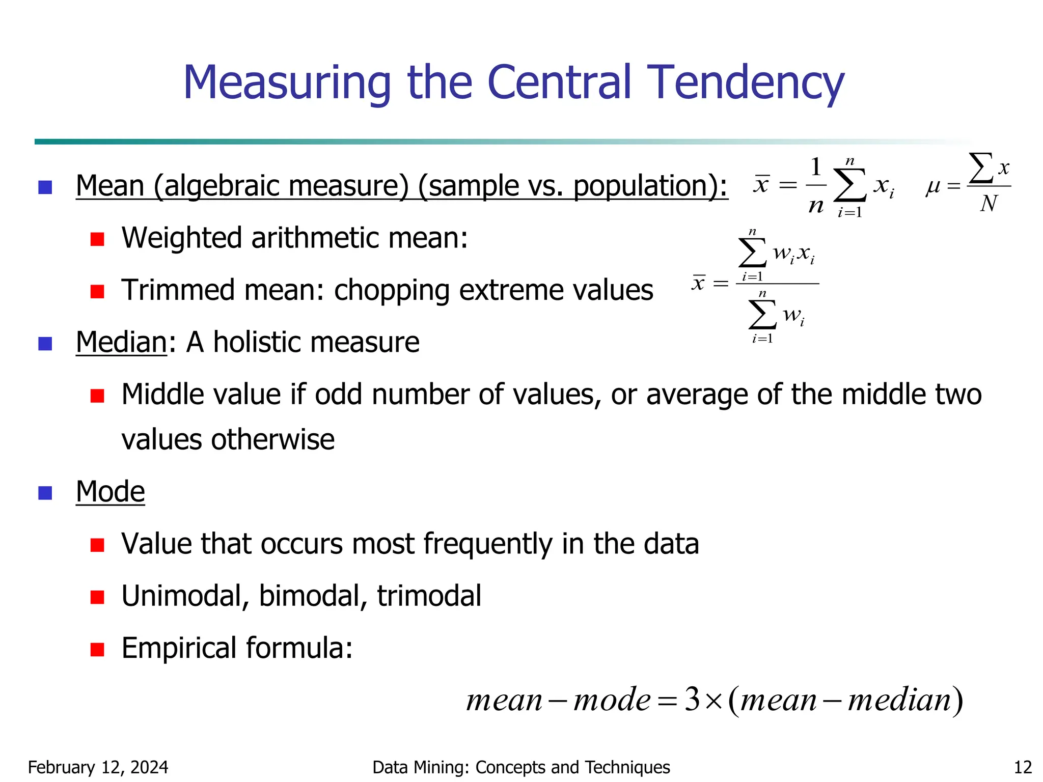
Measuring the Dispersion of Data
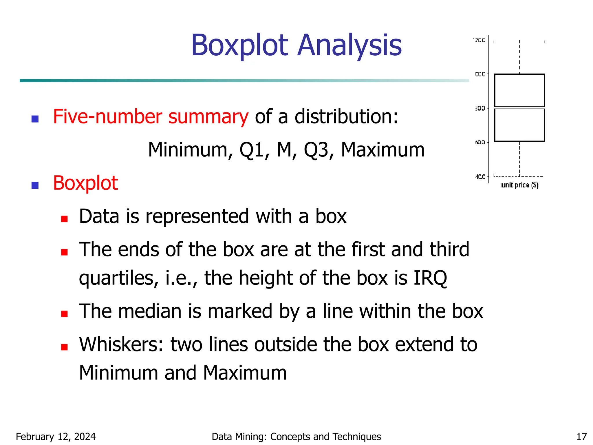
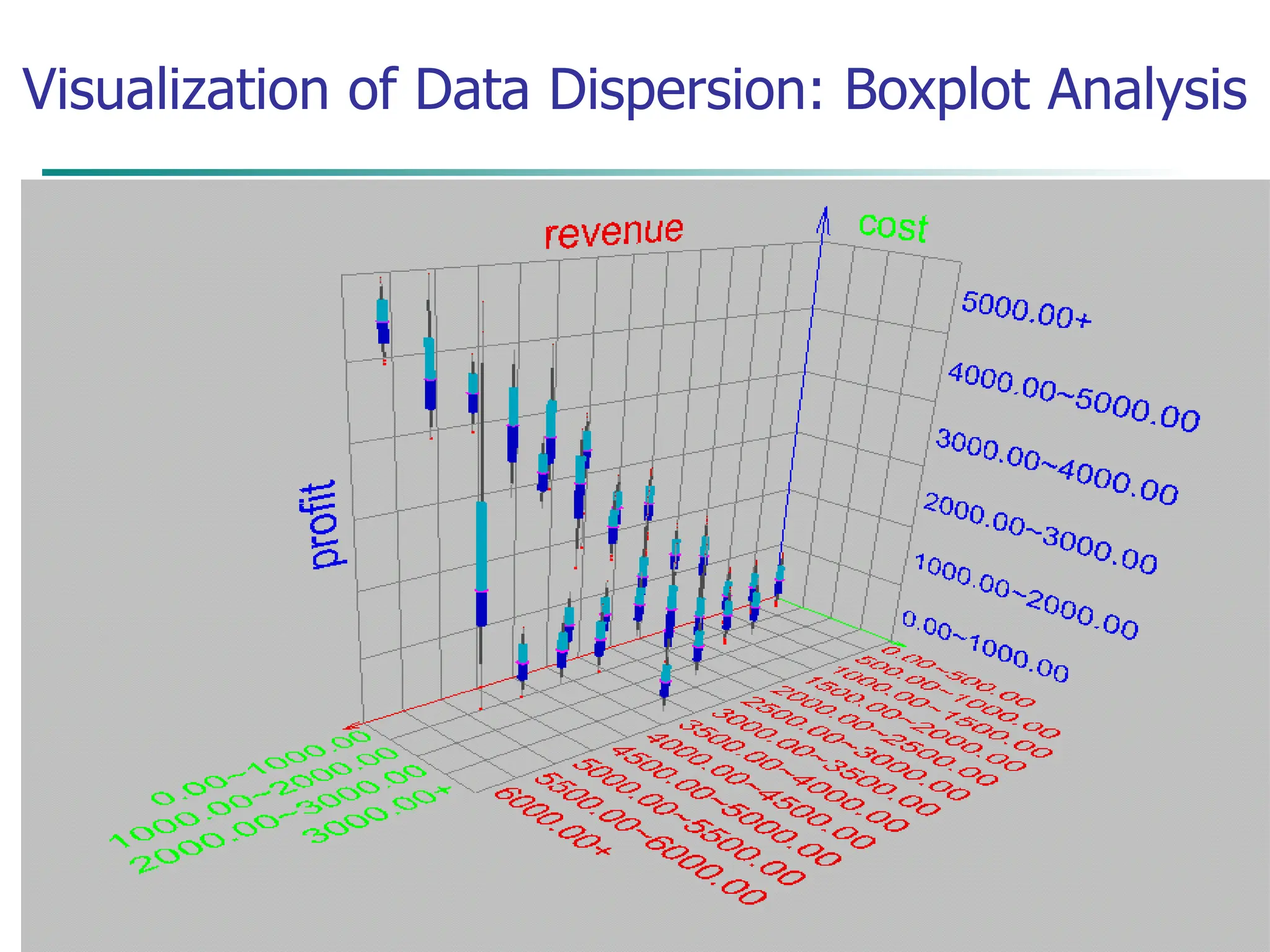
Quartiles, outliers and boxplots
Quartiles: Q1 (25th percentile), Q3 (75th percentile)
Inter-quartile range: IQR = Q3 – Q1
Five number summary: min, Q1, M, Q3, max
Boxplot: ends of the box are the quartiles, median is marked, whiskers (min
/ max), and plot outlier individually
Outlier: usually, a value higher/lower than 1.5 x IQR
Variance and standard deviation (sample: s, population: σ)
Variance: (algebraic, scalable computation)
Standard deviation s (or σ) is the square root of variance s2 (or σ2)
n
i
n
i
i
i
n
i
i x
n
x
n
x
x
n
s
1 1
2
2
1
2
2
]
)
(
1
[
1
1
)
(
1
1
n
i
i
n
i
i x
N
x
N 1
2
2
1
2
2 1
)
(
1
](https://image.slidesharecdn.com/chapter2datapreprocssing-240212204852-5e4c41bd/75/Transformacion-de-datos_Preprocssing-ppt-15-2048.jpg)
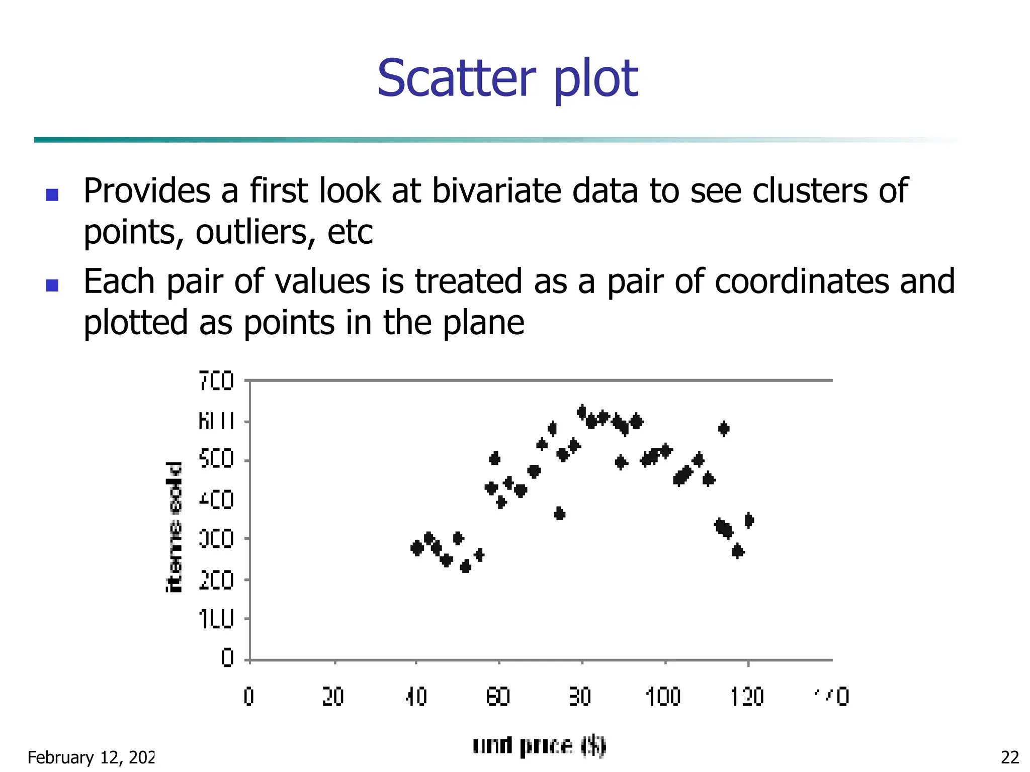
![February 12, 2024 Data Mining: Concepts and Techniques 20
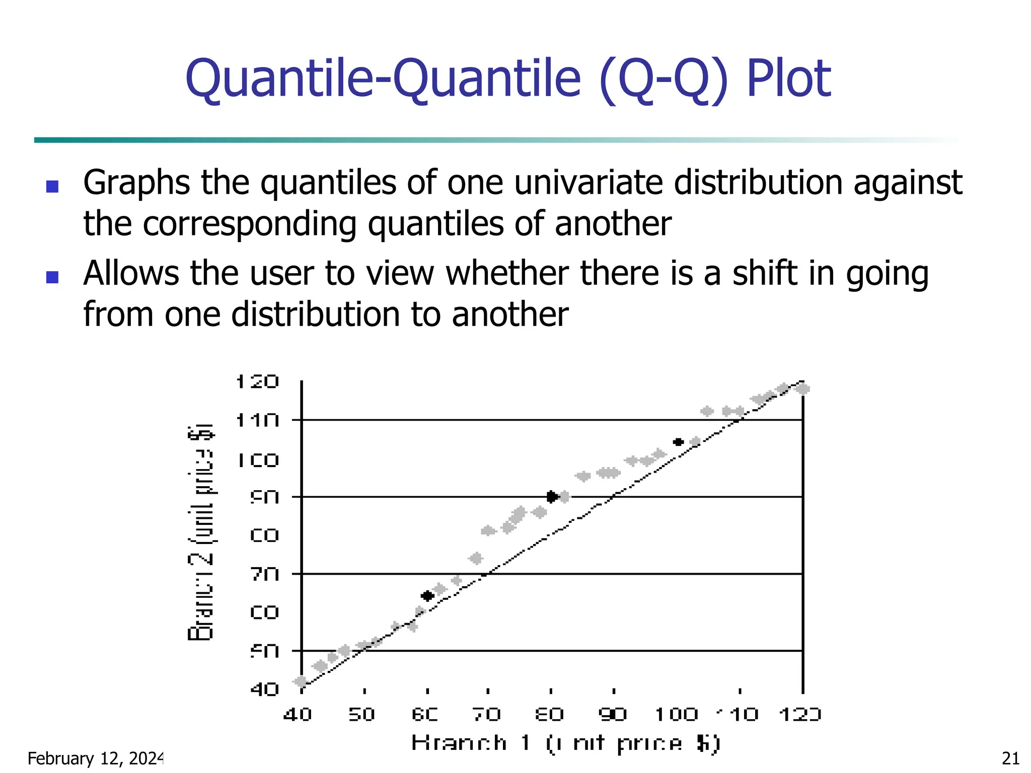
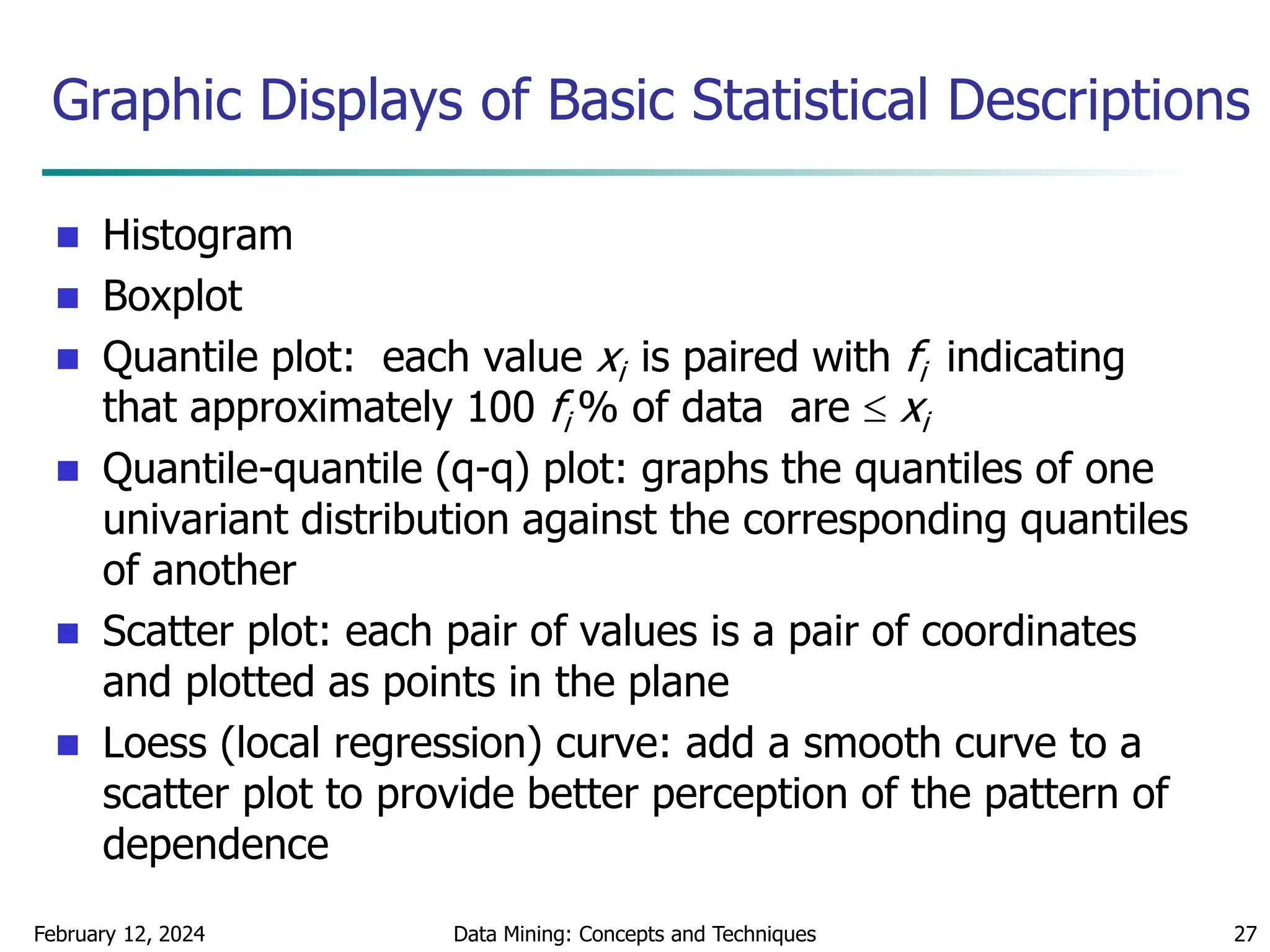
Quantile Plot
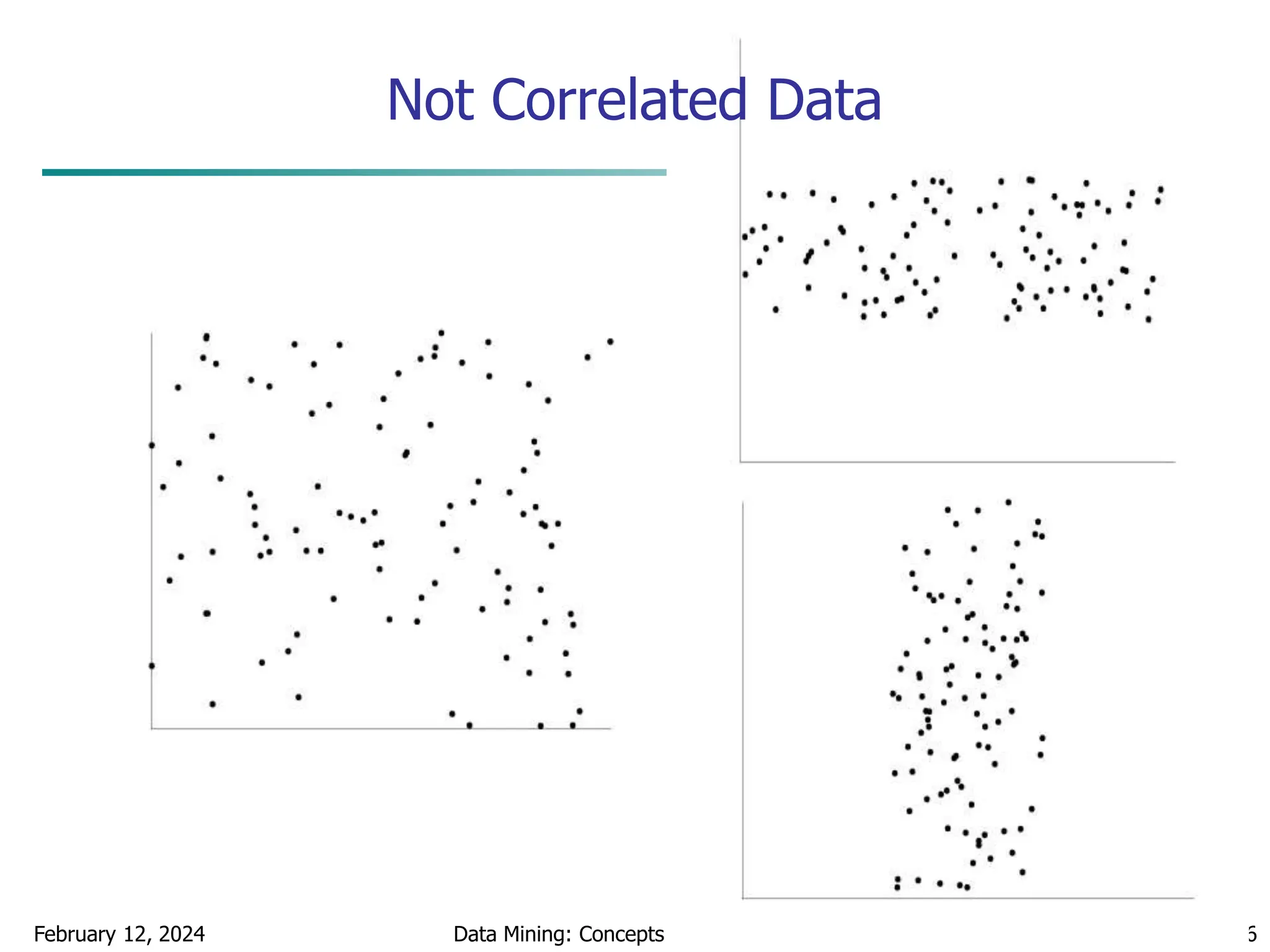
Displays all of the data (allowing the user to assess both
the overall behavior and unusual occurrences)
Plots quantile information
For a data xi data sorted in increasing order, fi in
range [0, 1] indicates that approximately 100 fi% of
the data are below or equal to the value xi](https://image.slidesharecdn.com/chapter2datapreprocssing-240212204852-5e4c41bd/75/Transformacion-de-datos_Preprocssing-ppt-20-2048.jpg)
![February 12, 2024 Data Mining: Concepts and Techniques 48
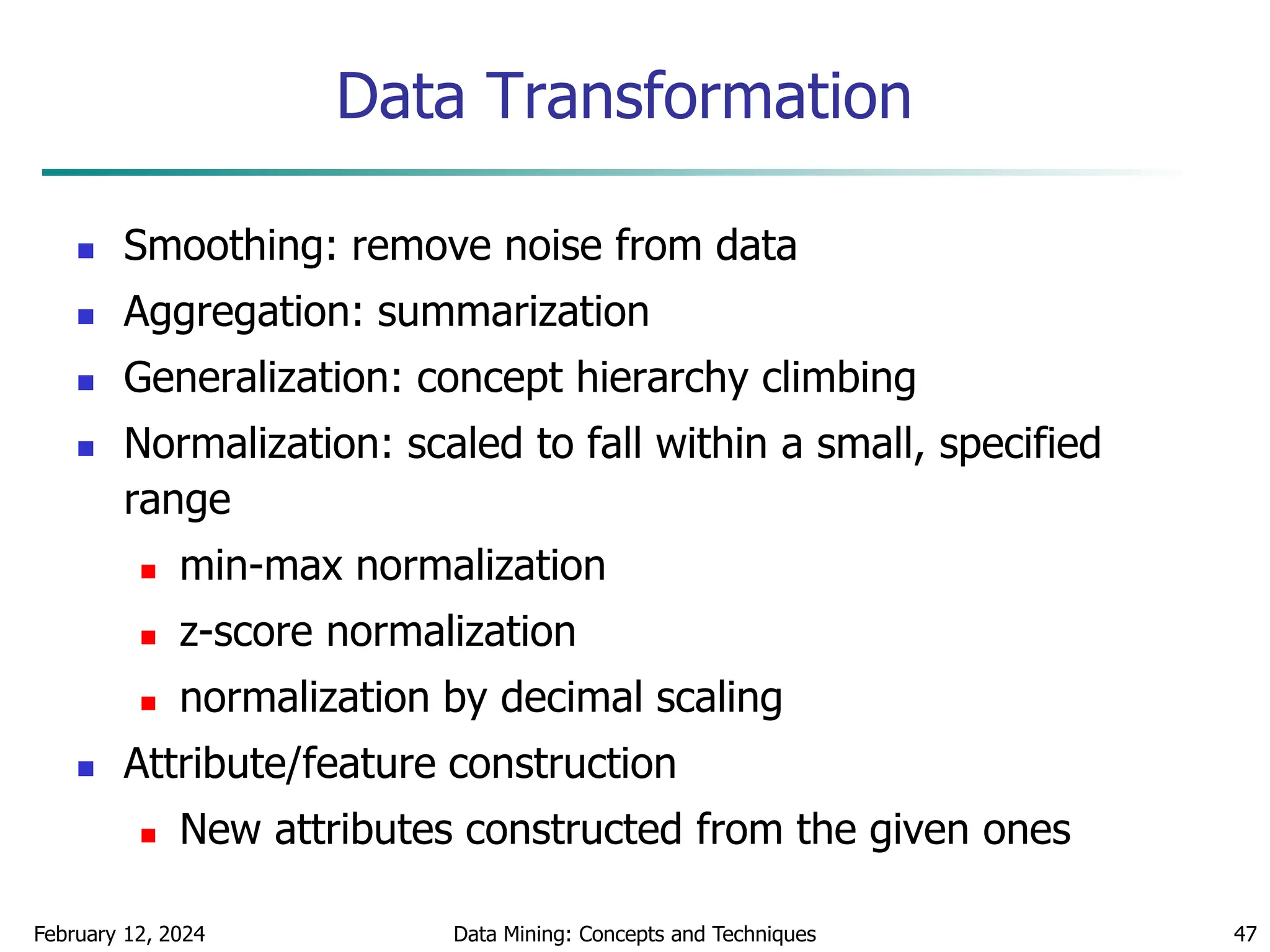
Data Transformation: Normalization
Min-max normalization: to [new_minA, new_maxA]
Ex. Let income range $12,000 to $98,000 normalized to [0.0,
1.0]. Then $73,000 is mapped to
Z-score normalization (μ: mean, σ: standard deviation):
Ex. Let μ = 54,000, σ = 16,000. Then
Normalization by decimal scaling
716
.
0
0
)
0
0
.
1
(
000
,
12
000
,
98
000
,
12
600
,
73
A
A
A
A
A
A
min
new
min
new
max
new
min
max
min
v
v _
)
_
_
(
'
A
A
v
v
'
j
v
v
10
' Where j is the smallest integer such that Max(|ν’|) < 1
225
.
1
000
,
16
000
,
54
600
,
73
](https://image.slidesharecdn.com/chapter2datapreprocssing-240212204852-5e4c41bd/75/Transformacion-de-datos_Preprocssing-ppt-48-2048.jpg)
![February 12, 2024 Data Mining: Concepts and Techniques 86
Interval Merge by 2 Analysis
Merging-based (bottom-up) vs. splitting-based methods
Merge: Find the best neighboring intervals and merge them to form
larger intervals recursively
ChiMerge [Kerber AAAI 1992, See also Liu et al. DMKD 2002]
Initially, each distinct value of a numerical attr. A is considered to be
one interval
2 tests are performed for every pair of adjacent intervals
Adjacent intervals with the least 2 values are merged together,
since low 2 values for a pair indicate similar class distributions
This merge process proceeds recursively until a predefined stopping
criterion is met (such as significance level, max-interval, max
inconsistency, etc.)](https://image.slidesharecdn.com/chapter2datapreprocssing-240212204852-5e4c41bd/75/Transformacion-de-datos_Preprocssing-ppt-86-2048.jpg)


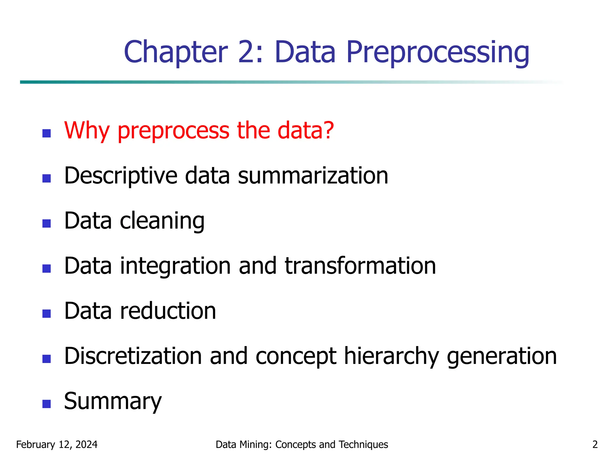
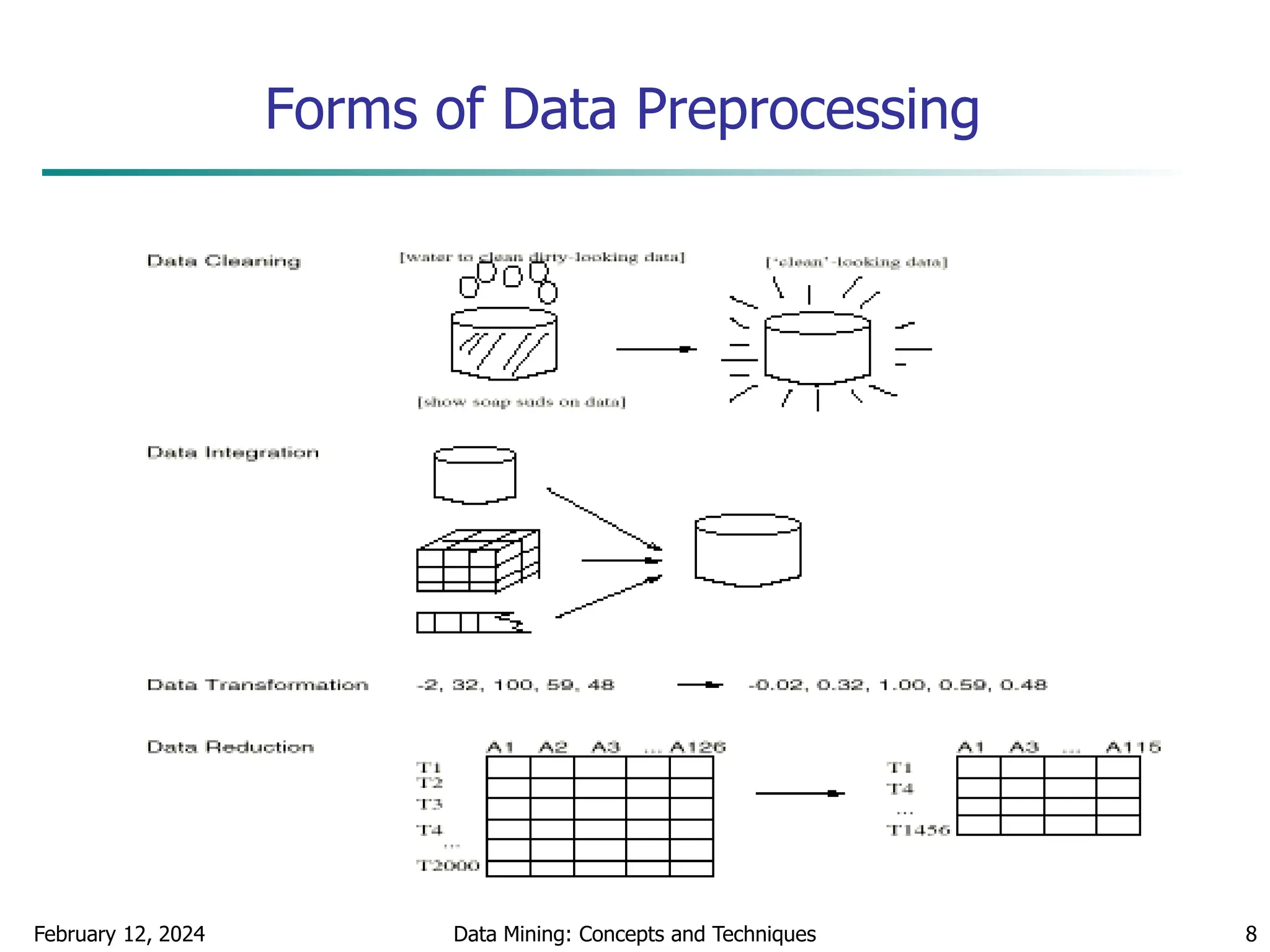
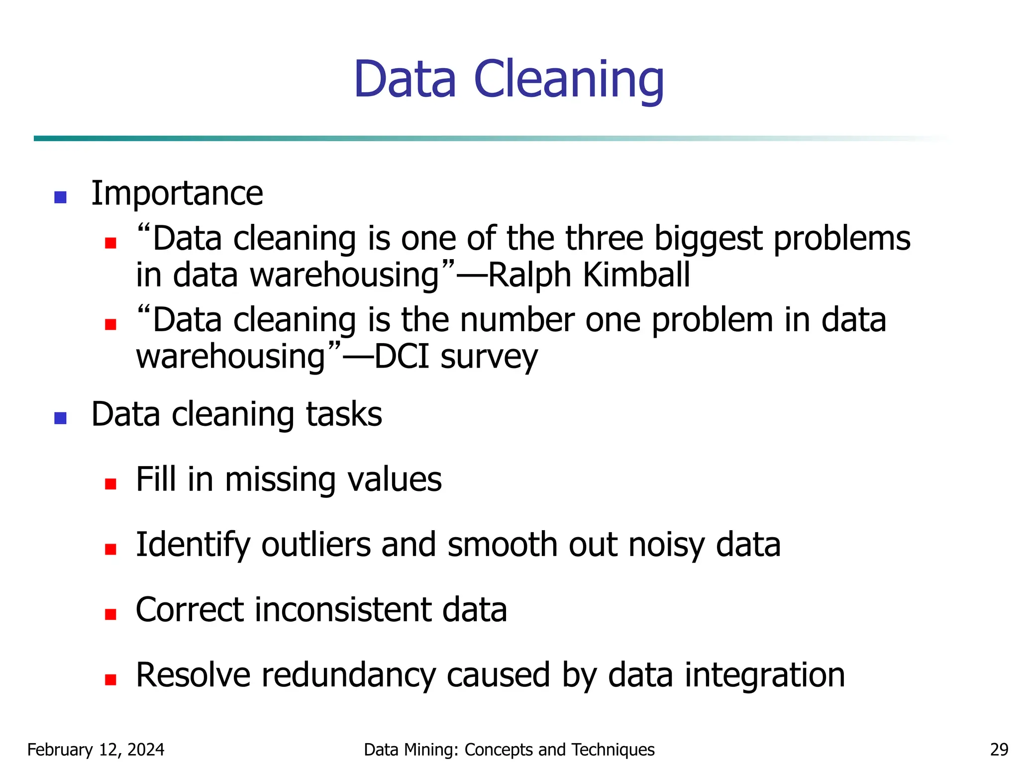
This document discusses data preprocessing techniques for data mining. It covers why preprocessing is important for obtaining quality data and mining results. The major tasks covered include data cleaning, integration, transformation, reduction, and discretization. Data cleaning techniques discussed include handling missing data, noisy data, and inconsistent data through methods like filling in values, smoothing, and resolving inconsistencies. Descriptive data analysis is also covered through statistical measures of central tendency, dispersion, and visualizations.