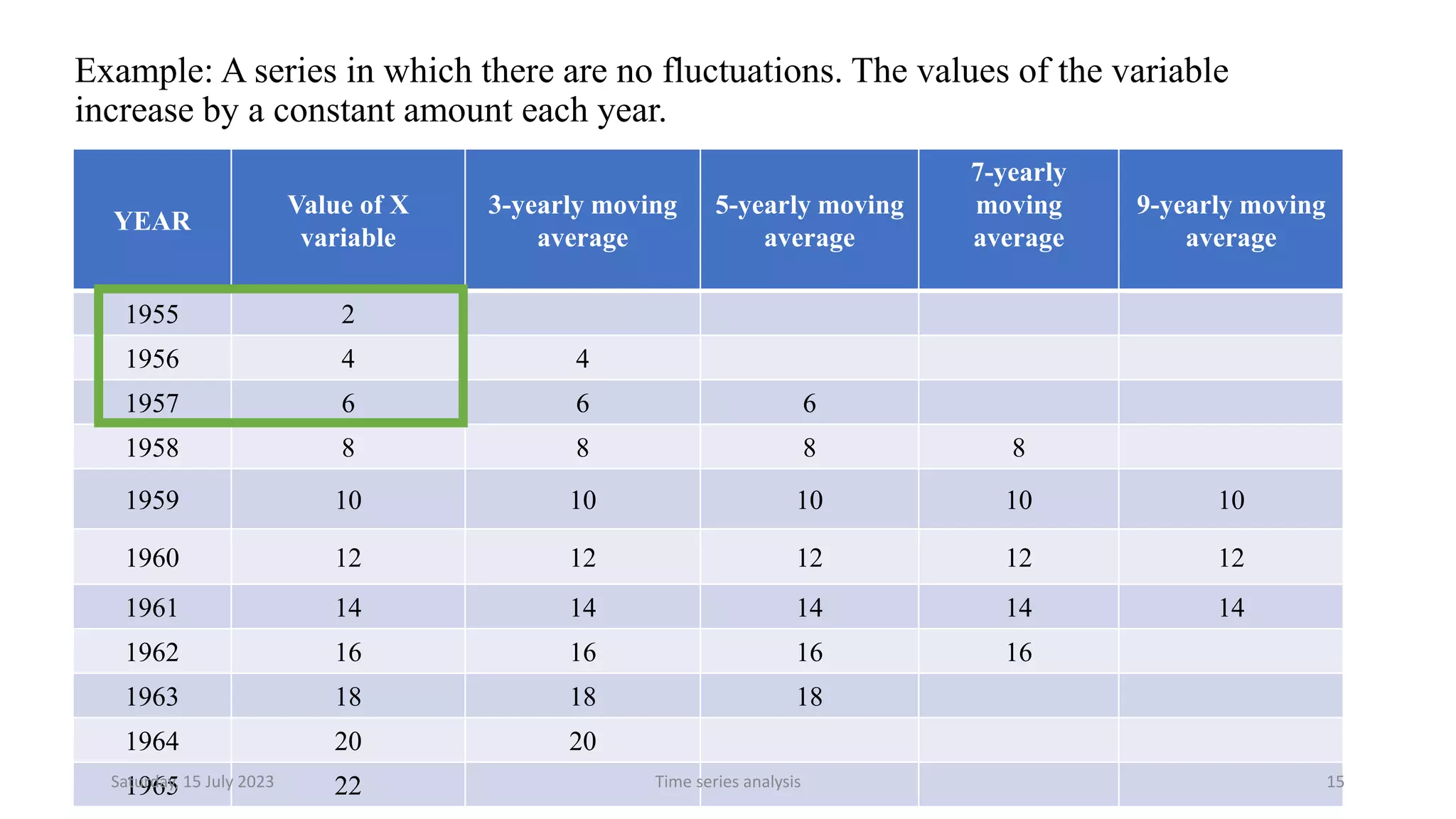
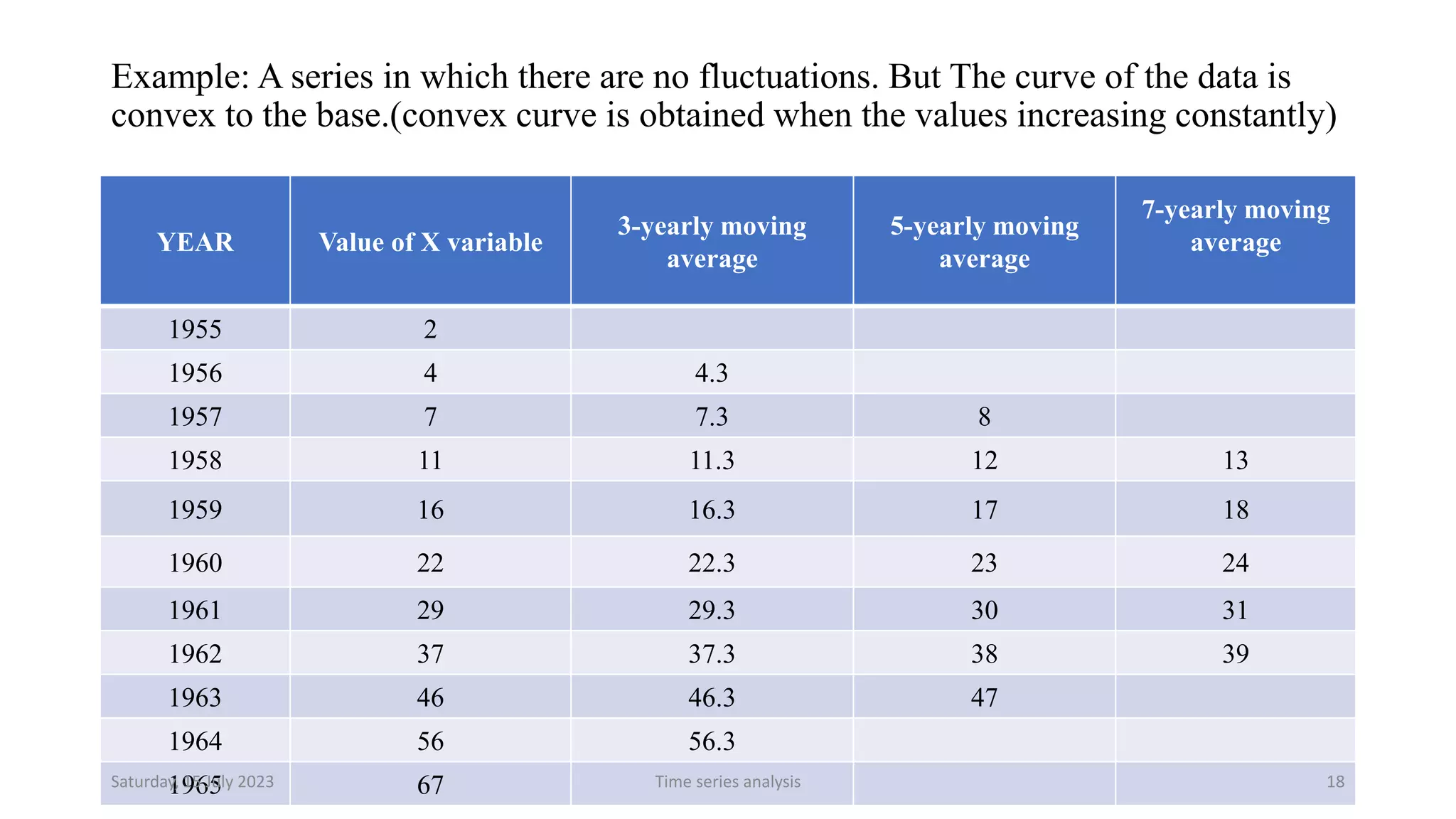
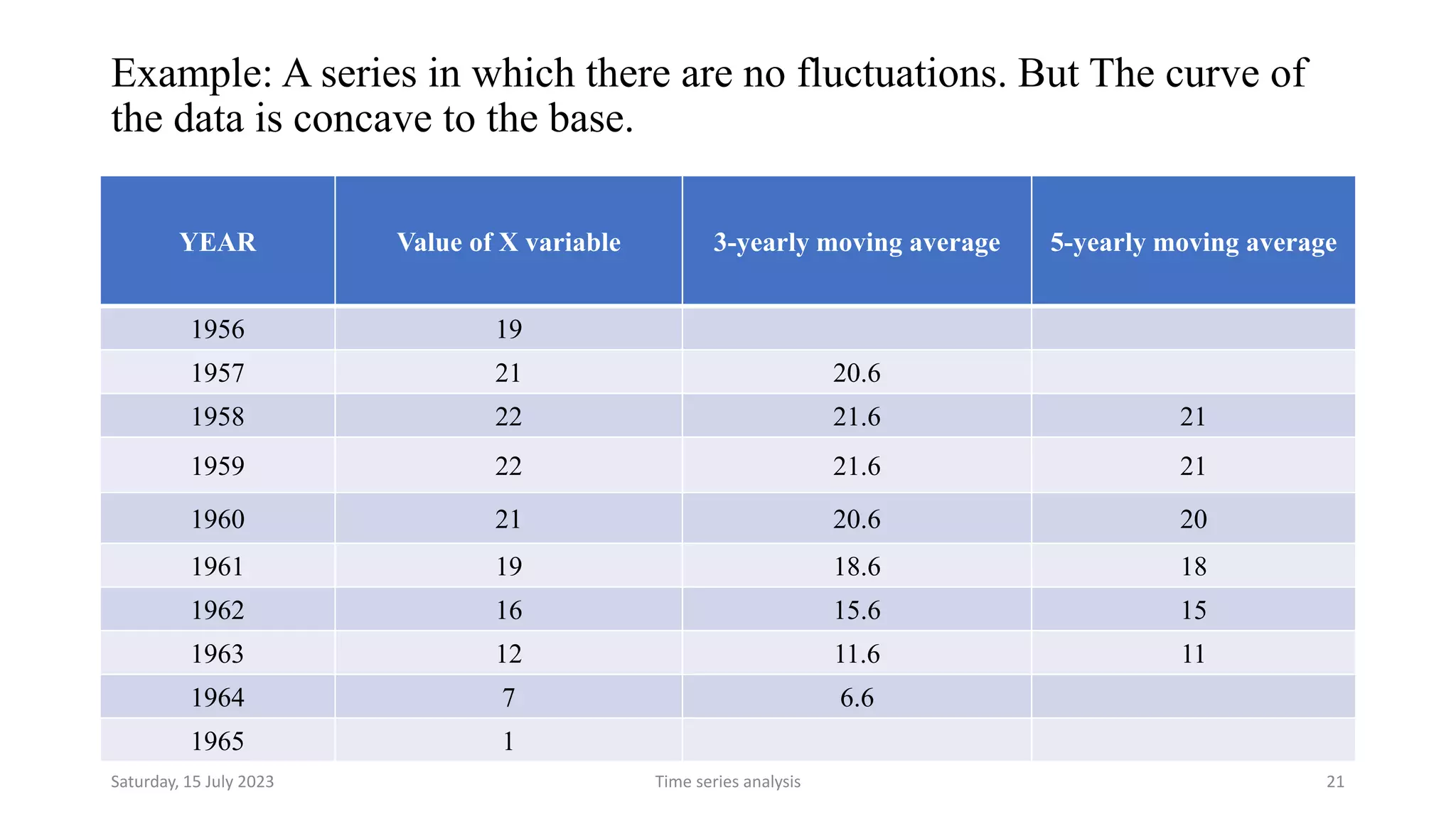
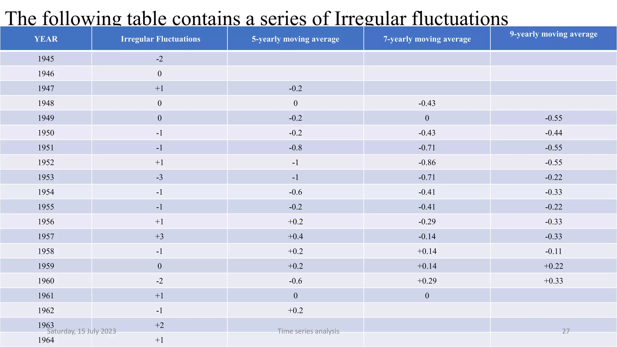
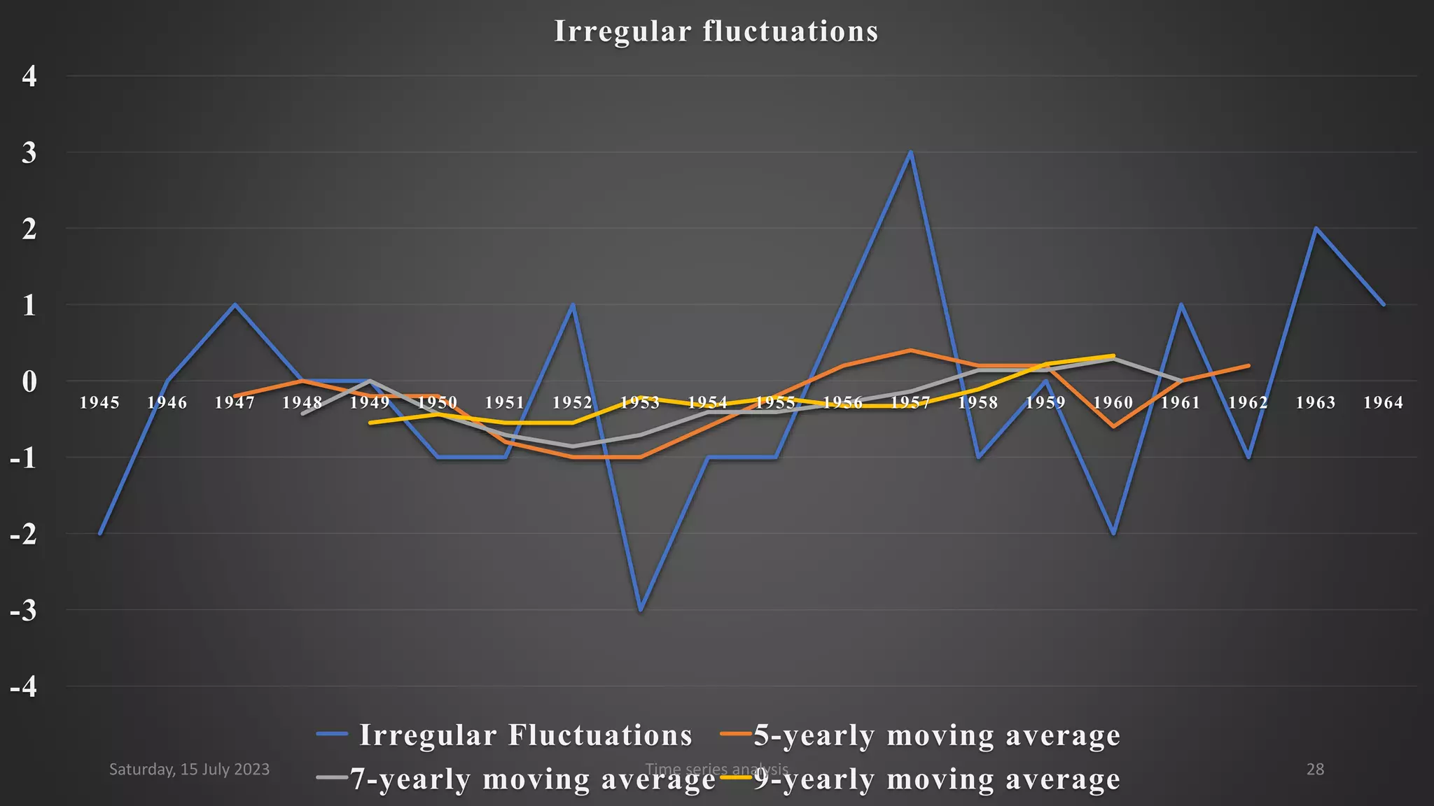
Time series analysis is a statistical methodology used to analyze longitudinal data measured over multiple time points. It can help understand the underlying process driving changes over time or evaluate the effects of interventions. Key components of time series include trends, seasonal variations, cyclical variations, and random variations. Moving average methods are commonly used to calculate trends and reduce other fluctuations in the data. Curve fitting by mathematical equations can also be used when the pattern of changes follows a known function.

1. Time series analysis

2. Time series analysis
• Time series analysis is a statistical methodology appropriate for an important class
of longitudinal research designs.
• Such designs typically involve single subjects or research units (e.g., incidence)
that are measured repeatedly at regular intervals over a large number of
observations.
• A time series analysis can help us to understand the underlying naturalistic
process, the pattern of change over time, or evaluate the effects of either a planned
or unplanned intervention.
Saturday, 15 July 2023 Time series analysis 2

3. Importance of time series analysis
1. Profit of experience
2. Safety from futures
3. Risk analysis and evaluation of changes
4. Utility studies, Budgetary analysis
5. Process and quality control
6. Inventory studies
7. Census analysis
8. Economic forecasting
9. Stock market analysis
Saturday, 15 July 2023 Time series analysis 3

4. Components of a time series
• Trend-values have a tendency to increase or decrease over time.
For example, the annual number of reported episodes of food poisoning has
increased over time.
• Seasonal variation-similar patterns appear in corresponding seasons in successive
years.
For example, hay fever rates show a distinct seasonal pattern.
• Cyclical variation-variation of any other fixed period.
For example, measurements may display a circadian pattern, with levels cycling
over a 24 h period.
• Random variation-variation that does not exhibit any fixed pattern over time
Saturday, 15 July 2023 Time series analysis 4

5. Saturday, 15 July 2023 Time series analysis 5

6. Secular trend
• The increase or decrease in the movements of a time series over a long period of time is
called secular trend.
• A time series data may show upward trend or downward trend for a period of years, and
this may be due to factors like:
1. Increase in population,
2. Change in technological progress,
3. Large scale shift in consumers demands,
for examples,
1. Population increases over a period of time, price increase over a period of years, production of
drugs, medical equipment's on the capital market of the country increases over a period of years.
these are the examples of upward trend.
2. The sales of a commodity may decrease over a period of time because of better products coming to
the market. this is an example of declining trend or downward.
Saturday, 15 July 2023 Time series analysis 6

7. Seasonal variation:
• Seasonal variation are short term fluctuation in a time series which occur
periodically in a year:
• This continues to repeat year after year.
• The major factors that are weather conditions (e.g., temperature, humidity, rainfall,
lifecycle of vectors, overcrowding).
• Seasonal variation in occurrence is a common feature of many diseases, especially
those of infectious origin.
• Studies of seasonal variation contribute to healthcare planning and to the
understanding of the etiology of infections.
Saturday, 15 July 2023 Time series analysis 7

8. Cyclical fluctuation:
• Cyclical variations are recurrent upward or downward movements in a time series,
but the period of cycle is mostly greater than a year.
• These variations are regular
• For example, measles in the pre-vaccination era appeared in cycles with major
peaks every 2-3 years and rubella every 6-9 years. This was due to naturally
occurring variations in herd immunity.
• Influenza pandemics are known to occur at intervals of 7- 10 years, due to
antigenic variations.
Saturday, 15 July 2023 Time series analysis 8

9. Irregular/Random Variation
• Irregular variations are fluctuation in time series that are short in duration, erratic in
nature and follow no regularity in the occurrence pattern.
• These variations are also referred what is left out in a time series after cyclical and
seasonal variations. Irregular fluctuations results due to the occurrence of unforeseen
events like:
1. Floods
2. Earthquakes
3. Wars
4. Famines
Saturday, 15 July 2023 Time series analysis 9

10. Analysing time series data
• We usually have one of two aims when studying time series data.
1. To understand the mechanism that generated the series in order to produce a model
that can be used to predict future values of the series.
2. To assess the impact of some exposure on the series, after taking account of
confounding variables.
• For example, we may wish to assess the impact of air pollution, measurements
which themselves form a time series, on the number of asthma attacks, after taking
account of daily weather conditions.
Saturday, 15 July 2023 Time series analysis 10

11. • If we are concerned with the relationship between two series which show a similar
trend (e.g. a seasonal trend, or a gradual increase over time), then the two series
will be correlated, even if there is no underlying causal relationship between them.
• For the purposes of analysis, we usually reduce our time series to a stationary
time series, in which there is no trend and cyclic variation does not increase or
decrease over time.
Saturday, 15 July 2023 Time series analysis 11

12. Measurement of trend:
• The following methods are used for calculation of trend :
1. Curve fitting by inspection
2. Moving average method
3. Curve fitting by mathematical equations.
Saturday, 15 July 2023 Time series analysis 12

13. Curve Fitting By Inspection
• In this method the data are first plotted on a graph paper and a smoothed curve is
plotted to the data merely by inspection.
• Such curves eliminate other component-regular and irregular fluctuations.
• This is the best method from the point of view of simplicity.
• Main disadvantage of this method is that the trend curve so drawn can be effected
by the bias of the statistician.
Saturday, 15 July 2023 Time series analysis 13

14. Moving Average Method:
• It is one of the most popular method for calculating long term trend.
• Moving average method is a simple device of reducing fluctuations and
obtaining trend values with a fair degree of accuracy.
• This method is also used for ‘Seasonal fluctuation', 'Cyclical fluctuation’ and
‘Irregular fluctuation’.
• In this method we calculate the ‘moving average for certain years.
• Trend values are affected by moving average period.
Saturday, 15 July 2023 Time series analysis 14

15. YEAR
Value of X
variable
3-yearly moving
average
5-yearly moving
average
7-yearly
moving
average
9-yearly moving
average
1955 2
1956 4 4
1957 6 6 6
1958 8 8 8 8
1959 10 10 10 10 10
1960 12 12 12 12 12
1961 14 14 14 14 14
1962 16 16 16 16
1963 18 18 18
1964 20 20
1965 22
Example: A series in which there are no fluctuations. The values of the variable
increase by a constant amount each year.
Saturday, 15 July 2023 Time series analysis 15

16. 0
5
10
15
20
25
1955 1956 1957 1958 1959 1960 1961 1962 1963 1964 1965
Linear trend
Value of X variable 3-yearly moving average 5-yearly moving average
7-yearly moving average 9-yearly moving average
Saturday, 15 July 2023 Time series analysis 16

17. • The above table gives a series in which there are no fluctuations.
• The values of the variable increase be a constant amount each year.
• If a series contains no fluctuations but only general trend, which when plotted on
a graph paper gives a straight line, the moving average will reproduce the series,
such trend is called linear trend.
• If the data were in a reverse order, then also the original series would have been
repeated with different period of moving averages however this time the trend
would have been downwards.
Saturday, 15 July 2023 Time series analysis 17

18. Example: A series in which there are no fluctuations. But The curve of the data is
convex to the base.(convex curve is obtained when the values increasing constantly)
YEAR Value of X variable
3-yearly moving
average
5-yearly moving
average
7-yearly moving
average
1955 2
1956 4 4.3
1957 7 7.3 8
1958 11 11.3 12 13
1959 16 16.3 17 18
1960 22 22.3 23 24
1961 29 29.3 30 31
1962 37 37.3 38 39
1963 46 46.3 47
1964 56 56.3
1965 67
Saturday, 15 July 2023 Time series analysis 18

19. 0
10
20
30
40
50
60
70
80
1955 1956 1957 1958 1959 1960 1961 1962 1963 1964 1965
Curvi-linear trend (convex to the base)
Value of X variable 3-yearly moving average
5-yearly moving average 7-yearly moving average
Saturday, 15 July 2023 Time series analysis 19

20. • Moving average figure have given curves which are parallel to the curve of the
original data, but all these curves are above the original curve.
• Trend value are more than the original values.
• Greater the period of moving average the farther the trend curve is from the curve
of the original data
Saturday, 15 July 2023 Time series analysis 20

21. Example: A series in which there are no fluctuations. But The curve of
the data is concave to the base.
YEAR Value of X variable 3-yearly moving average 5-yearly moving average
1956 19
1957 21 20.6
1958 22 21.6 21
1959 22 21.6 21
1960 21 20.6 20
1961 19 18.6 18
1962 16 15.6 15
1963 12 11.6 11
1964 7 6.6
1965 1
Saturday, 15 July 2023 Time series analysis 21

22. 0
5
10
15
20
25
1956 1957 1958 1959 1960 1961 1962 1963 1964 1965
Curvi-linear trend (concave to the base)
Value of X variable 3-yearly moving average 5-yearly moving average
Saturday, 15 July 2023 Time series analysis 22

23. • These curves are below the curve of the original series indicating that in such
cases trend values are less than the original ones.
• Moving average figure have given curves which are parallel to the curve of the
original data
• Greater the period of moving average the farther the trend curve is from the curve
of the original data
Saturday, 15 July 2023 Time series analysis 23

24. The following table contains a series of regular fluctuations
YEAR regular Fluctuations 5-yearly moving average 7-yearly moving average
9-yearly moving average
1945 2
1946 2
1947 0 0.2
1948 -1 -0.6 0
1949 -2 -0.8 0 0.4
1950 -2 -0.4 0 0.2
1951 1 0.2 0 -0.1
1952 2 0.6 0 -0.3
1953 2 0.8 0 -0.4
1954 0 0.2 0 -0.1
1955 -1 -0.6 0 0.3
1956 -2 -0.8 0 0.4
1957 -2 -0.4 0 0.2
1958 1 0.2 0 -0.1
1959 2 0.6 0 -0.3
1960 2 0.8 0 -0.4
1961 0 0.2 0
1962 -1 -0.6
1963 -2
1964 -2
Saturday, 15 July 2023 Time series analysis 24

25. -2.5
-2
-1.5
-1
-0.5
0
0.5
1
1.5
2
2.5
1945 1946 1947 1948 1949 1950 1951 1952 1953 1954 1955 1956 1957 1958 1959 1960 1961 1962 1963 1964
Cyclical fluctuation and their moving average
fluctuations 5-yearly moving average
7-yearly moving average 9-yearly moving average
Saturday, 15 July 2023 Time series analysis 25

26. • If a series contains cyclical fluctuations a moving average with a period less or
more than the period of the cycle would only reduce the fluctuations, but if the
period of the moving average is the same as the period of the cycle or its multiple
the fluctuations would be completely eliminated.
• Moving average with a period coinciding with the period of cycle in a series or its
multiple eliminates cyclical fluctuations, while moving averages with periods less
than or more than it only reduce them.
Saturday, 15 July 2023 Time series analysis 26

27. The following table contains a series of Irregular fluctuations
YEAR Irregular Fluctuations 5-yearly moving average 7-yearly moving average
9-yearly moving average
1945 -2
1946 0
1947 +1 -0.2
1948 0 0 -0.43
1949 0 -0.2 0 -0.55
1950 -1 -0.2 -0.43 -0.44
1951 -1 -0.8 -0.71 -0.55
1952 +1 -1 -0.86 -0.55
1953 -3 -1 -0.71 -0.22
1954 -1 -0.6 -0.41 -0.33
1955 -1 -0.2 -0.41 -0.22
1956 +1 +0.2 -0.29 -0.33
1957 +3 +0.4 -0.14 -0.33
1958 -1 +0.2 +0.14 -0.11
1959 0 +0.2 +0.14 +0.22
1960 -2 -0.6 +0.29 +0.33
1961 +1 0 0
1962 -1 +0.2
1963 +2
1964 +1
Saturday, 15 July 2023 Time series analysis 27

28. -4
-3
-2
-1
0
1
2
3
4
1945 1946 1947 1948 1949 1950 1951 1952 1953 1954 1955 1956 1957 1958 1959 1960 1961 1962 1963 1964
Irregular fluctuations
Irregular Fluctuations 5-yearly moving average
7-yearly moving average 9-yearly moving average
Saturday, 15 July 2023 Time series analysis 28

29. • Moving average cannot eliminate irregular fluctuations. It only reduces them and
upto certain limit, the longer the period of moving average the greater would be
the reduction, after a certain limit an increase in the period of moving average will
increase the fluctuation also.
Saturday, 15 July 2023 Time series analysis 29

30. Curve fitting by mathematical equations:
• If the increase or decrease in the values of a particular series is of equal absolute
amount year after year, or, if the increase or decrease is always a constant
percentage, as in case of compound interest sums, it is better to establish
mathematical equations of the increase or decrease, and to fit a trend based on the
values obtained by such equations.
• In mathematical curves, it is presumed that there is a definite law which governs
the changes and as such, the trend values so obtained on the equation representing
this law rather than on the data themselves.
Saturday, 15 July 2023 Time series analysis 30

31. • Moving average method is in this case more flexible because if the data change,
the moving average also changes.
• In mathematical case of mathematical curve unless the equation is changed, the
trend values would not change.
• If a series relating to the production of coal conforms to a particular mathematical
equation and if it is found that due to new discoveries in the technique of coal
production that equation no more holds good, a new equation may have to be
established.
Saturday, 15 July 2023 Time series analysis 31

32. Measurement of seasonal fluctuations:
1. Method of monthly averages to compute the seasonal variation index.
2. Method of moving averages to compute seasonal variations and indices of
seasonal variations.
3. Method of link relatives.
Saturday, 15 July 2023 Time series analysis 32

33. Measurement of cyclical and irregular
fluctuations:
• If from the original series trend and seasonal variations are isolated the remainder
consist of cyclical and irregular fluctuations.
• There is no well recognised method of separating irregular and cyclical
fluctuations.
• One method is by finding out the moving average of the series of cyclical irregular
fluctuations. By this fluctuations irregular fluctuations would be reduced, and
cyclical data would become more prominent.
Saturday, 15 July 2023 Time series analysis 33

34. • The more irregular series is, the longer should be the period of moving average so
that irregularities in one direction may be set off against irregularities in another
direction.
• After removing trend, seasonal, cyclical fluctuations from original data whatever
remains continues the irregular fluctuations.
• There is no method to isolate the irregular fluctuations.
Saturday, 15 July 2023 Time series analysis 34

35. Other methods of analysing time series:
1. Fitting straight line trend- method of least squares
2. Fitting a curve of the power series
3. The correlogram
- Autocorrelation
4. The periodogram
5. Autoregressive Integrated Moving Average (ARIMA) models
Saturday, 15 July 2023 Time series analysis 35

36. Reference
1. Fundamentals of statistics
2. Medical statistics at a glance- aviva Petrie & caroline sabin
3. Statistics in medicine
4. Park 26th edition
5. Velicer, W. F., & Fava, J. L. (2003). Time Series Analysis. In J. Schinka & W. F.
Velicer (Eds.), Research Methods in Psychology(581-606). Volume 2, Handbook
of Psychology (I. B. Weiner, Editor-in-Chief.). New York: John Wiley & Sons.
Saturday, 15 July 2023 Time series analysis 36

37. Thank you
37