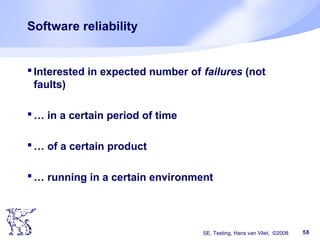
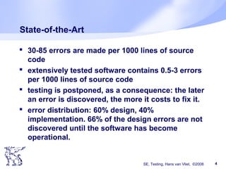
The document discusses software testing techniques. It notes that many errors occur early in the development process but are often discovered late, which makes them costly to fix. Testing should therefore start early. Various testing techniques are discussed, including manual techniques like inspections, as well as coverage-based techniques that aim to cover all statements, branches, and paths in the code. Testing should aim to find as many faults as possible while also increasing confidence that the software works correctly. Starting testing activities early in the development lifecycle can help reduce costs associated with fixing errors.


![SE, Testing, Hans van Vliet, ©2008 16
Example constructive approach
Task: test module that sorts an array A[1..n]. A
contains integers; n < 1000
Solution: take n = 0, 1, 37, 999, 1000. For n = 37,
999, take A as follows:
A contains random integers
A contains increasing integers
A contains decreasing integers
These are equivalence classes: we assume that
one element from such a class suffices
This works if the partition is perfect](https://image.slidesharecdn.com/testingppt-160620201202/85/Testingppt-16-320.jpg)


![SE, Testing, Hans van Vliet, ©2008 30
Example of control-flow coverage
procedure bubble (var a: array [1..n] of integer; n: integer);
var i, j: temp: integer;
begin
for i:= 2 to n do
if a[i] >= a[i-1] then goto next endif;
j:= i;
loop: if j <= 1 then goto next endif;
if a[j] >= a[j-1] then goto next endif;
temp:= a[j]; a[j]:= a[j-1]; a[j-1]:= temp; j:= j-1; goto loop;
next: skip;
enddo
end bubble;
input: n=2, a[1] = 5, a[2] = 3
√
√
√
√
√
√
√
√
√
√
√
√](https://image.slidesharecdn.com/testingppt-160620201202/85/Testingppt-30-320.jpg)
![SE, Testing, Hans van Vliet, ©2008 31
Example of control-flow coverage (cnt’d)
procedure bubble (var a: array [1..n] of integer; n: integer);
var i, j: temp: integer;
begin
for i:= 2 to n do
if a[i] >= a[i-1] then goto next endif;
j:= i;
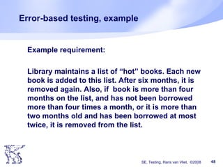
loop: if j <= 1 then goto next endif;
if a[j] >= a[j-1] then goto next endif;
temp:= a[j]; a[j]:= a[j-1]; a[j-1]:= temp; j:= j-1; goto loop;
next: skip;
enddo
end bubble;
input: n=2, a[1] = 5, a[2] = 3
√
√
√
√
√
√
√
√
√
√
√
√
a[i]=a[i-1]](https://image.slidesharecdn.com/testingppt-160620201202/85/Testingppt-31-320.jpg)


![SE, Testing, Hans van Vliet, ©2008 40
Mutation testing
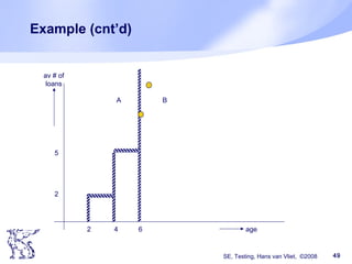
procedure insert(a, b, n, x);
begin bool found:= false;
for i:= 1 to n do
if a[i] = x
then found:= true; goto leave endif
enddo;
leave:
if found
then b[i]:= b[i] + 1
else n:= n+1; a[n]:= x; b[n]:= 1
endif
end insert;
2
-
n-1](https://image.slidesharecdn.com/testingppt-160620201202/85/Testingppt-40-320.jpg)
![SE, Testing, Hans van Vliet, ©2008 41
Mutation testing (cnt’d)
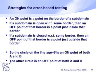
procedure insert(a, b, n, x);
begin bool found:= false;
for i:= 1 to n do
if a[i] = x
then found:= true; goto leave endif
enddo;
leave:
if found
then b[i]:= b[i] + 1
else n:= n+1; a[n]:= x; b[n]:= 1
endif
end insert;
n-1](https://image.slidesharecdn.com/testingppt-160620201202/85/Testingppt-41-320.jpg)
![SE, Testing, Hans van Vliet, ©2008 42
How tests are treated by mutants
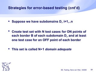
Let P be the original, and P’ the mutant
Suppose we have two tests:
T1 is a test, which inserts an element that equals a[k] with
k<n
T2 is another test, which inserts an element that does not
equal an element a[k] with k<n
Now P and P’ will behave the same on T1, while
they differ for T2
In some sense, T2 is a “better” test, since it in a
way tests this upper bound of the for-loop, which
T1 does not](https://image.slidesharecdn.com/testingppt-160620201202/85/Testingppt-42-320.jpg)