1 Null andAlternative Hypotheses
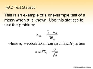
2 Test Statistic
3 P-Value
4 Significance Level
5 One-Sample z Test
6 Power and Sample Size
3.
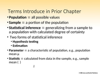
Terms Introduce inPrior Chapter
•Population all possible values
•Sample a portion of the population
•Statistical inference generalizing from a sample to
a population with calculated degree of certainty
• Two forms of statistical inference
• Hypothesis testing
• Estimation
• Parameter a characteristic of population, e.g., population
mean µ
• Statistic calculated from data in the sample, e.g., sample
mean ( )
x
4.
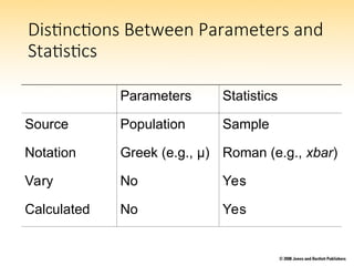
Distinctions Between Parametersand
Statistics
Parameters Statistics
Source Population Sample
Notation Greek (e.g., μ) Roman (e.g., xbar)
Vary No Yes
Calculated No Yes
6.
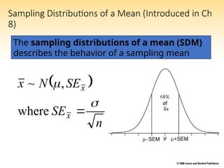
Sampling Distributions ofa Mean (Introduced in Ch
8)
n
SE
SE
N
x
x
x
where
,
~
The sampling distributions of a mean (SDM)
describes the behavior of a sampling mean
7.
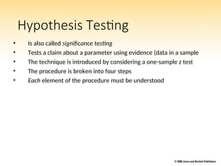
Hypothesis Testing
• Isalso called significance testing
• Tests a claim about a parameter using evidence (data in a sample
• The technique is introduced by considering a one-sample z test
• The procedure is broken into four steps
• Each element of the procedure must be understood
8.
Hypothesis Testing Steps
A.Null and alternative hypotheses
B. Test statistic
C. P-value and interpretation
D. Significance level (optional)
9.
§9.1 Null andAlternative Hypotheses
• Convert the research question to null and alternative hypotheses
• The null hypothesis (H0) is a claim of “no difference in the population”
• The alternative hypothesis (Ha) claims “H0 is false”
• Collect data and seek evidence against H0 as a way of bolstering Ha
(deduction)
10.
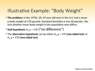
Illustrative Example: “BodyWeight”
• The problem: In the 1970s, 20–29 year old men in the U.S. had a mean
μ body weight of 170 pounds. Standard deviation σ was 40 pounds. We
test whether mean body weight in the population now differs.
• Null hypothesis H0: μ = 170 (“no difference”)
• The alternative hypothesis can be either Ha: μ > 170 (one-sided test) or
Ha: μ ≠ 170 (two-sided test)
Illustrative Example: zstatistic
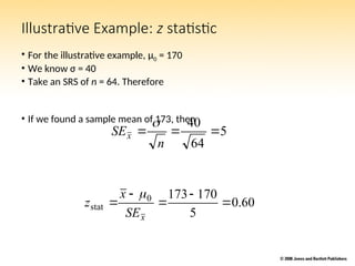
• For the illustrative example, μ0 = 170
• We know σ = 40
• Take an SRS of n = 64. Therefore
• If we found a sample mean of 173, then
5
64
40
n
SEx
60
.
0
5
170
173
0
stat
x
SE
x
z
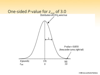
13.
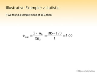
Illustrative Example: zstatistic
If we found a sample mean of 185, then
00
.
3
5
170
185
0
stat
x
SE
x
z
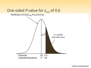
§9.3 P-value
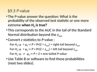
•The P-valueanswer the question: What is the
probability of the observed test statistic or one more
extreme when H0 is true?
•This corresponds to the AUC in the tail of the Standard
Normal distribution beyond the zstat.
•Convert z statistics to P-value :
For Ha: μ> μ0 P = Pr(Z > zstat) = right-tail beyond zstat
For Ha: μ< μ0 P = Pr(Z < zstat) = left tail beyond zstat
For Ha: μμ0 P = 2 × one-tailed P-value
•Use Table B or software to find these probabilities
(next two slides).
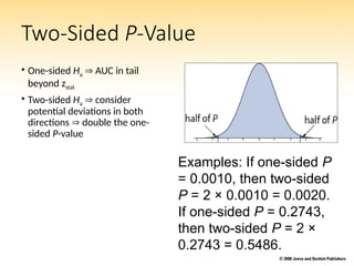
Two-Sided P-Value
• One-sidedHa AUC in tail
beyond zstat
• Two-sided Ha consider
potential deviations in both
directions double the one-
sided P-value
Examples: If one-sided P
= 0.0010, then two-sided
P = 2 × 0.0010 = 0.0020.
If one-sided P = 0.2743,
then two-sided P = 2 ×
0.2743 = 0.5486.
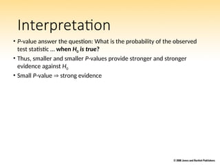
19.
Interpretation
• P-value answerthe question: What is the probability of the observed
test statistic … when H0 is true?
• Thus, smaller and smaller P-values provide stronger and stronger
evidence against H0
• Small P-value strong evidence
20.
Interpretation
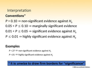
Conventions*
P > 0.10 non-significant evidence against H0
0.05 < P 0.10 marginally significant evidence
0.01 < P 0.05 significant evidence against H0
P 0.01 highly significant evidence against H0
Examples
P =.27 non-significant evidence against H0
P =.01 highly significant evidence against H0
* It is unwise to draw firm borders for “significance”
21.
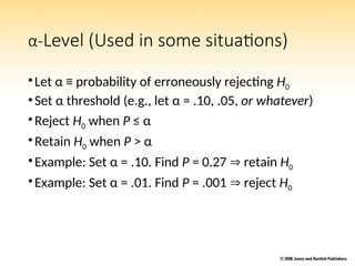
α-Level (Used insome situations)
•Let α ≡ probability of erroneously rejecting H0
•Set α threshold (e.g., let α = .10, .05, or whatever)
•Reject H0 when P ≤ α
•Retain H0 when P > α
•Example: Set α = .10. Find P = 0.27 retain H0
•Example: Set α = .01. Find P = .001 reject H0
22.
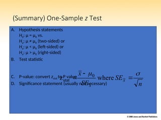
(Summary) One-Sample zTest
A. Hypothesis statements
H0: µ = µ0 vs.
Ha: µ ≠ µ0 (two-sided) or
Ha: µ < µ0 (left-sided) or
Ha: µ > µ0 (right-sided)
B. Test statistic
C. P-value: convert zstat to P value
D. Significance statement (usually not necessary) n
SE
SE
x
x
x
where
z 0
stat
23.
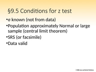
§9.5 Conditions forz test
•σ known (not from data)
•Population approximately Normal or large
sample (central limit theorem)
•SRS (or facsimile)
•Data valid
24.
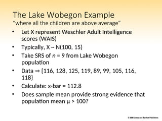
The Lake WobegonExample
“where all the children are above average”
• Let X represent Weschler Adult Intelligence
scores (WAIS)
• Typically, X ~ N(100, 15)
• Take SRS of n = 9 from Lake Wobegon
population
• Data {116, 128, 125, 119, 89, 99, 105, 116,
118}
• Calculate: x-bar = 112.8
• Does sample mean provide strong evidence that
population mean μ > 100?
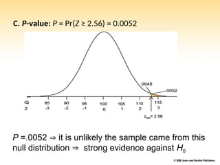
C. P-value: P= Pr(Z ≥ 2.56) = 0.0052
P =.0052 it is unlikely the sample came from this
null distribution strong evidence against H0
27.
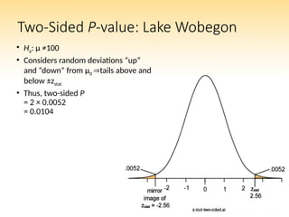
Two-Sided P-value: LakeWobegon
• Ha: µ ≠100
• Considers random deviations “up”
and “down” from μ0 tails above and
below ±zstat
• Thus, two-sided P
= 2 × 0.0052
= 0.0104
28.
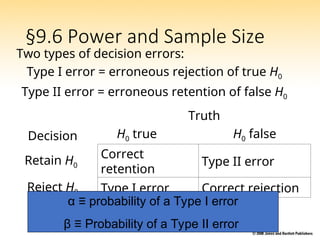
§9.6 Power andSample Size
Truth
Decision H0 true H0 false
Retain H0
Correct
retention
Type II error
Reject H0 Type I error Correct rejection
α ≡ probability of a Type I error
β ≡ Probability of a Type II error
Two types of decision errors:
Type I error = erroneous rejection of true H0
Type II error = erroneous retention of false H0
29.
Power
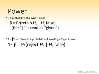
• β ≡probability of a Type II error
β = Pr(retain H0 | H0 false)
(the “|” is read as “given”)
• 1 – β “Power” ≡ probability of avoiding a Type II error
1– β = Pr(reject H0 | H0 false)
30.
Power of az test
where
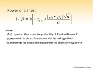
• Φ(z) represent the cumulative probability of Standard Normal Z
• μ0 represent the population mean under the null hypothesis
• μa represents the population mean under the alternative hypothesis
n
z a |
|
1 0
1 2
31.
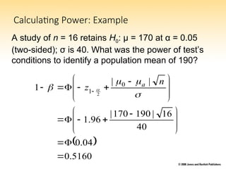
Calculating Power: Example
Astudy of n = 16 retains H0: μ = 170 at α = 0.05
(two-sided); σ is 40. What was the power of test’s
conditions to identify a population mean of 190?
5160
.
0
04
.
0
40
16
|
190
170
|
96
.
1
|
|
1 0
1 2
n
z a
32.
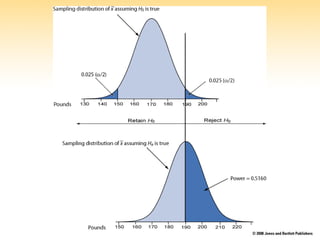
Reasoning Behind Power
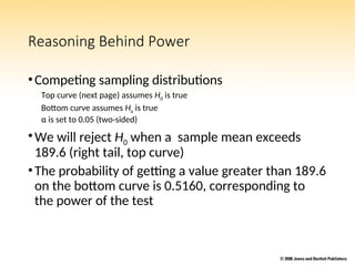
•Competingsampling distributions
Top curve (next page) assumes H0 is true
Bottom curve assumes Ha is true
α is set to 0.05 (two-sided)
•We will reject H0 when a sample mean exceeds
189.6 (right tail, top curve)
•The probability of getting a value greater than 189.6
on the bottom curve is 0.5160, corresponding to
the power of the test
34.
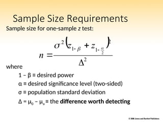
Sample Size Requirements
Samplesize for one-sample z test:
where
1 – β ≡ desired power
α ≡ desired significance level (two-sided)
σ ≡ population standard deviation
Δ = μ0 – μa ≡ the difference worth detecting
2
2
1
1
2
2
z
z
n
35.
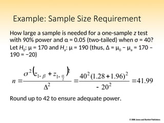
Example: Sample SizeRequirement
How large a sample is needed for a one-sample z test
with 90% power and α = 0.05 (two-tailed) when σ = 40?
Let H0: μ = 170 and Ha: μ = 190 (thus, Δ = μ0 − μa = 170 –
190 = −20)
Round up to 42 to ensure adequate power.
99
.
41
20
)
96
.
1
28
.
1
(
40
2
2
2
2
2
1
1
2
2
z
z
n
#3 Hypothesis testing is one of the two common forms of statistical inference. This slide reviews some of the terms that form the basis of statistical inference, as introduced in the prior chapter. Make certain you understand these basics before proceeding.
#4 This slide address an other foundation of statistical inference: the difference between parameters and statistics. Parameters and statistics are related, but are not the same thing.
Over the years teaching statistics, I have derived a hypothesis that explains why some students have difficulty with statistical inference: they fail to distinguish between statistics and parameter. When a student calculates a statistic such as a sample mean, it seems so tangible and real that they view it as a constant. I think they would be better off if they recognized a statistic as merely one example of what might have been had they done the study or experiment at a different time.
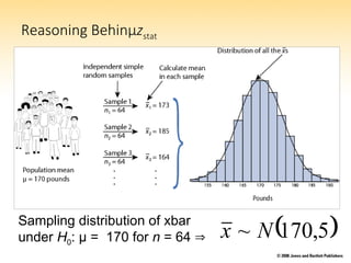
#6 This slide summarize what we’ve learned about the sampling distribution of a mean from a large sample. It is based no three important sampling postulates: the central limit theorem, the law of large numbers (unbiased nature of the sample mean), and square root law. Based on these well established statistical theorems we can say that means based on large samples (and means based in Normal populations) will have a Normal sampling distribution with an expectation equal to the population mean with a standard deviation equal to the standard deviation of the population divided by the square root of the sample size n.
#7 Hypothesis testing (also called significance testing) uses a quasi-deductive procedure to judge claims about parameters. Before testing a statistical hypothesis it is important to clearly state the nature of the claim to be tested. We are then going to use a four step procedure (as outlined in the last bullet) to test the claim.
#9 The first step in the procedure is to state the hypotheses null and alternative forms. The null hypothesis (abbreviate “H naught”) is a statement of no difference. The alternative hypothesis (“H sub a”) is a statement of difference. Seek evidence against the claim of H0 as a way of bolstering Ha.
The next slide offers an illustrative example on setting up the hypotheses.
#10 In the late 1970s, the weight of U.S. men between 20- and 29-years of age had a log-normal distribution with a mean of 170 pounds and standard deviation of 40 pounds. As you know, the overweight and obese conditions seems to be more prevalent today, constituting a major public health problem. To illustrate the hypothesis testing procedure, we ask if body weight in this group has increased since 1970. Under the null hypothesis there is no difference in the mean body weight between then and now, in which case μ would still equal 170 pounds.
Under the alternative hypothesis, the mean weight has increased Therefore, Ha: μ > 170. This statement of the alternative hypothesis is one-sided. That is, it looks only for values larger than stated under the null hypothesis.
There is another way to state the alternative hypothesis. We could state it in a “two-sided” manner, looking for values that are either higher- or lower-than expected. For the current illustrative example, the two-sided alternative is Ha: μ ≠ 170. Although for the current illustrative example, this seems unnecessary, two-sided alternative offers several advantages and are much more common in practice.