Download as PDF, PPTX


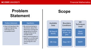
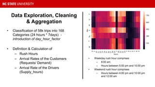
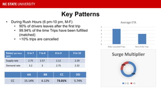
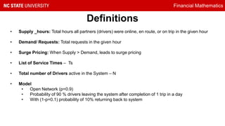
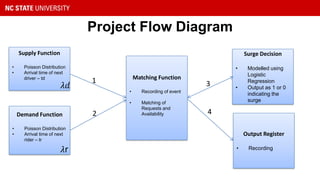
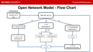
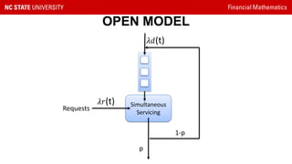
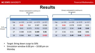
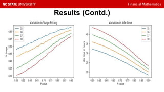


This document presents a study on reducing surge pricing for cab hailing services during rush hours. It analyzes data from 58,000 taxi trips over 28 days to identify rush hour periods between 6-10pm Monday through Friday with high demand. An open network Poisson model is used to simulate driver and rider arrival rates. The model shows communicating rush hour timing and locations to drivers can decrease surge pricing by up to 10% by motivating more drivers to continue working during these periods. However, the assumptions require validation and driver psychology was not fully considered. Future work could focus on demand-supply equilibrium and behavioral factors.


