Statistics and its measures with Python

1. Doing Stats with Python Way
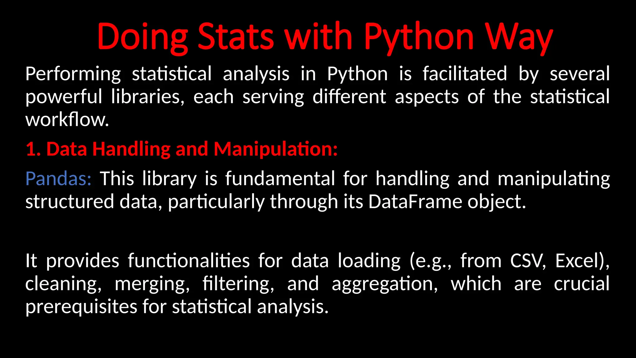
Performing statistical analysis in Python is facilitated by several
powerful libraries, each serving different aspects of the statistical
workflow.
1. Data Handling and Manipulation:
Pandas: This library is fundamental for handling and manipulating
structured data, particularly through its DataFrame object.
It provides functionalities for data loading (e.g., from CSV, Excel),
cleaning, merging, filtering, and aggregation, which are crucial
prerequisites for statistical analysis.

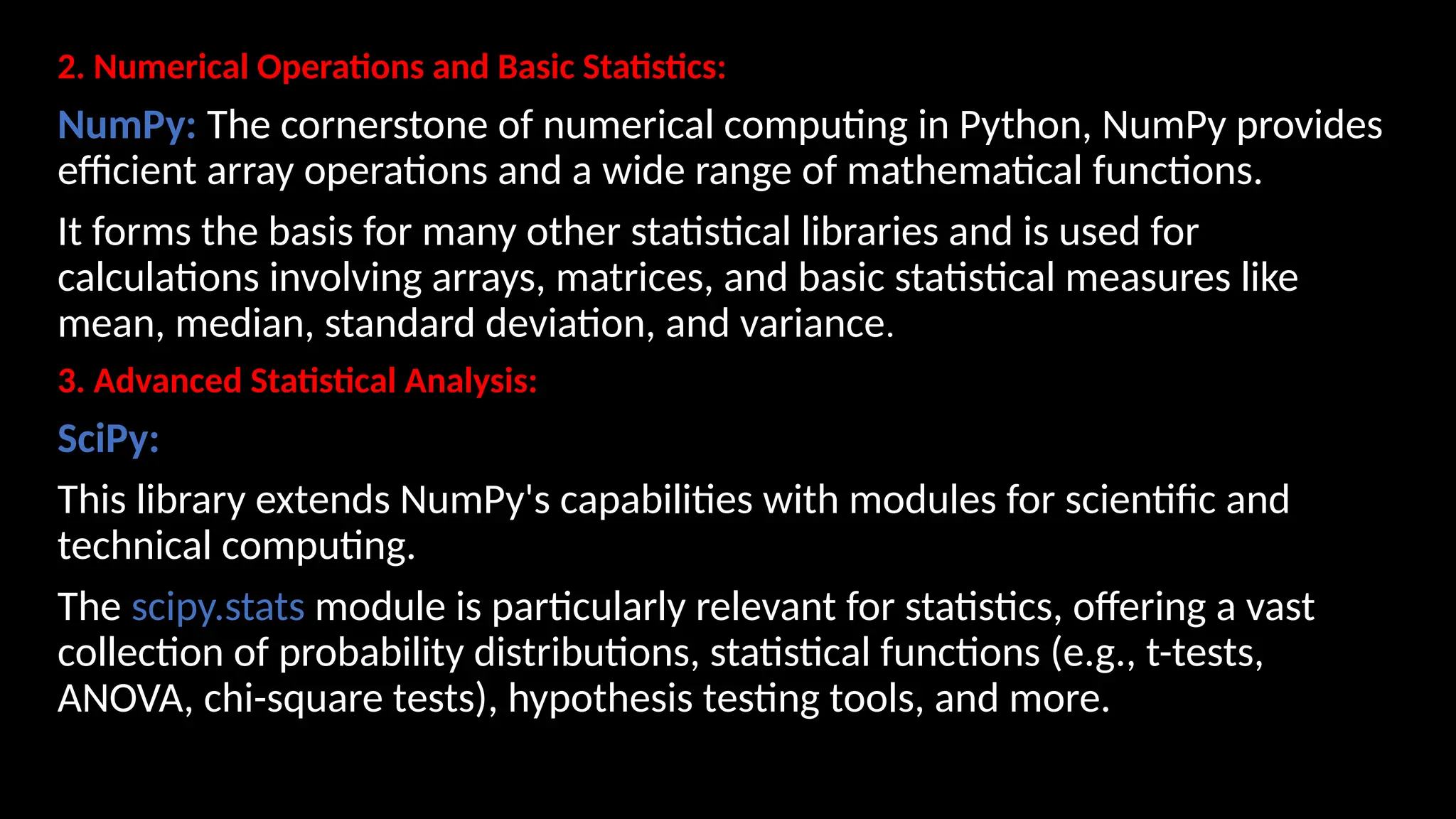
2. 2. Numerical Operations and Basic Statistics:
NumPy: The cornerstone of numerical computing in Python, NumPy provides
efficient array operations and a wide range of mathematical functions.
It forms the basis for many other statistical libraries and is used for
calculations involving arrays, matrices, and basic statistical measures like
mean, median, standard deviation, and variance.
3. Advanced Statistical Analysis:
SciPy:
This library extends NumPy's capabilities with modules for scientific and
technical computing.
The scipy.stats module is particularly relevant for statistics, offering a vast
collection of probability distributions, statistical functions (e.g., t-tests,
ANOVA, chi-square tests), hypothesis testing tools, and more.

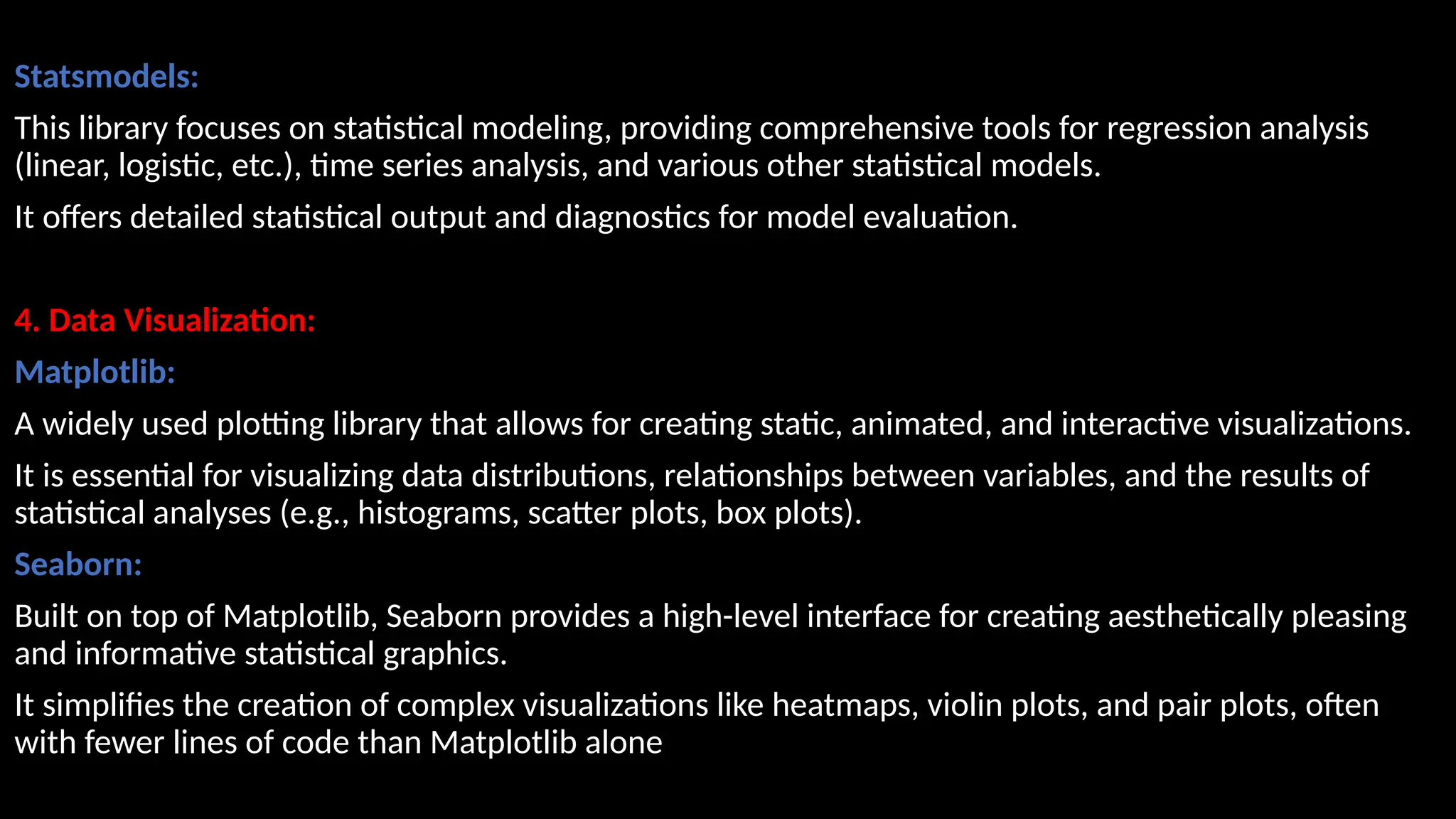
3. Statsmodels:
This library focuses on statistical modeling, providing comprehensive tools for regression analysis
(linear, logistic, etc.), time series analysis, and various other statistical models.
It offers detailed statistical output and diagnostics for model evaluation.
4. Data Visualization:
Matplotlib:
A widely used plotting library that allows for creating static, animated, and interactive visualizations.
It is essential for visualizing data distributions, relationships between variables, and the results of
statistical analyses (e.g., histograms, scatter plots, box plots).
Seaborn:
Built on top of Matplotlib, Seaborn provides a high-level interface for creating aesthetically pleasing
and informative statistical graphics.
It simplifies the creation of complex visualizations like heatmaps, violin plots, and pair plots, often
with fewer lines of code than Matplotlib alone

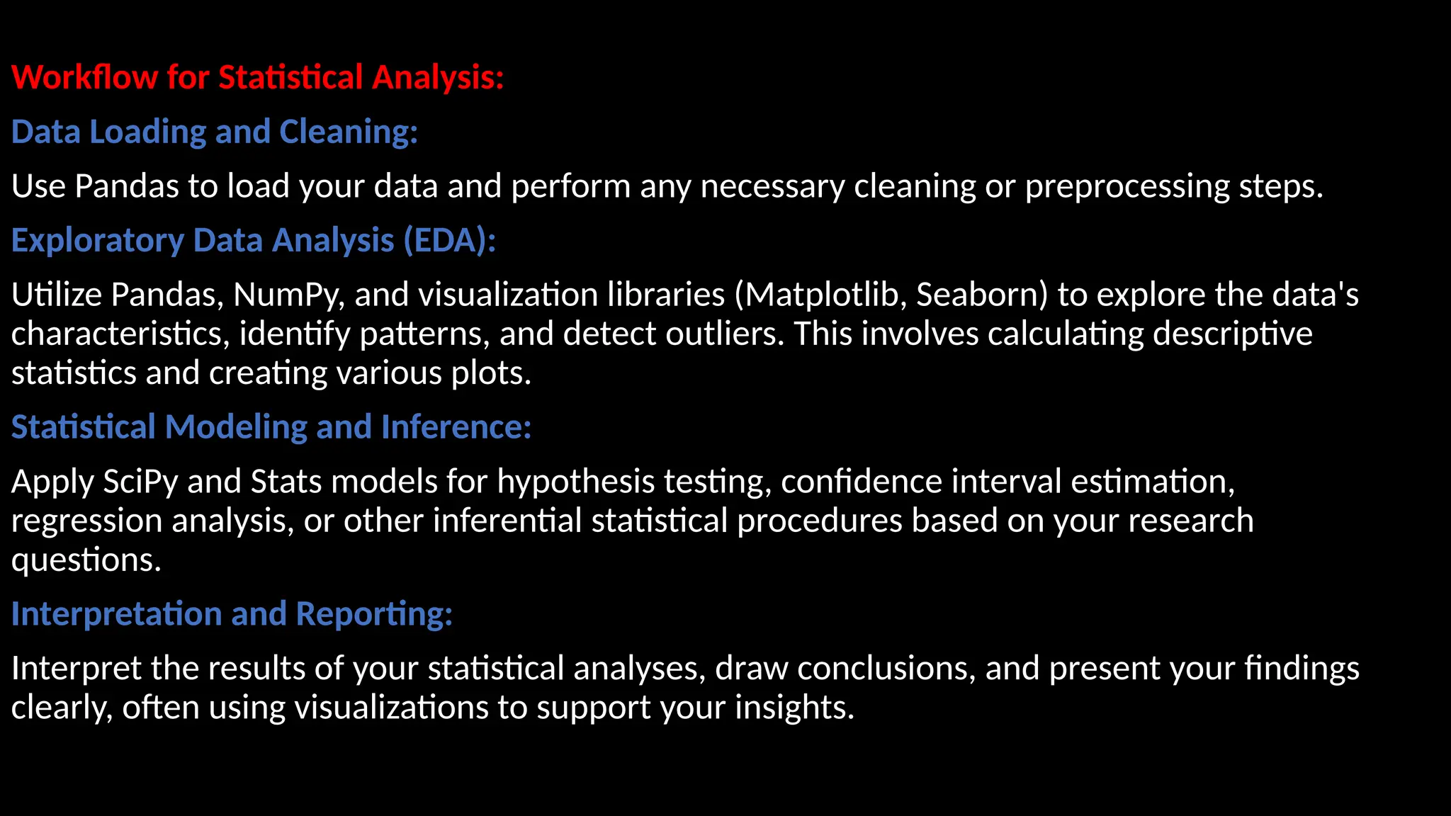
4. Workflow for Statistical Analysis:
Data Loading and Cleaning:
Use Pandas to load your data and perform any necessary cleaning or preprocessing steps.
Exploratory Data Analysis (EDA):
Utilize Pandas, NumPy, and visualization libraries (Matplotlib, Seaborn) to explore the data's
characteristics, identify patterns, and detect outliers. This involves calculating descriptive
statistics and creating various plots.
Statistical Modeling and Inference:
Apply SciPy and Stats models for hypothesis testing, confidence interval estimation,
regression analysis, or other inferential statistical procedures based on your research
questions.
Interpretation and Reporting:
Interpret the results of your statistical analyses, draw conclusions, and present your findings
clearly, often using visualizations to support your insights.

5. # Python code to demonstrate the working of mean()
# Python code to demonstrate the working of mean()
# importing statistics to handle statistical operations
import statistics
#initializing list
li = [1, 2, 3, 3, 2, 2, 2, 1]
# using mean() to calculate average of list
print ("The average of list values is : ",end="")
print (statistics.mean(li))
from statistics import median
data1 = (2, 3.5, 4, 5, 7, 9)
print("Median of data-set 1 is % s" % (median(data1)))
print("Low Median of the set is % s "
%(statistics.median_low(data1)))

6. Median_High:
set1 = [1, 3, 3, 4, 5, 7]
print("Median of the set is %s"
% (statistics.median(set1)))
# Print high median of the data-set
print("High Median of the set is %s "
% (statistics.median_high(set1)))

7. Mode
It is the value that has the highest frequency in the given data set.
The data set may have no mode if the frequency of all data points is the same.
Also, we can have more than one mode if we encounter two or more data points having
the same frequency.
The mode() function returns the number with the maximum number of occurrences. If the
passed argument is empty, StatisticsError is raised.

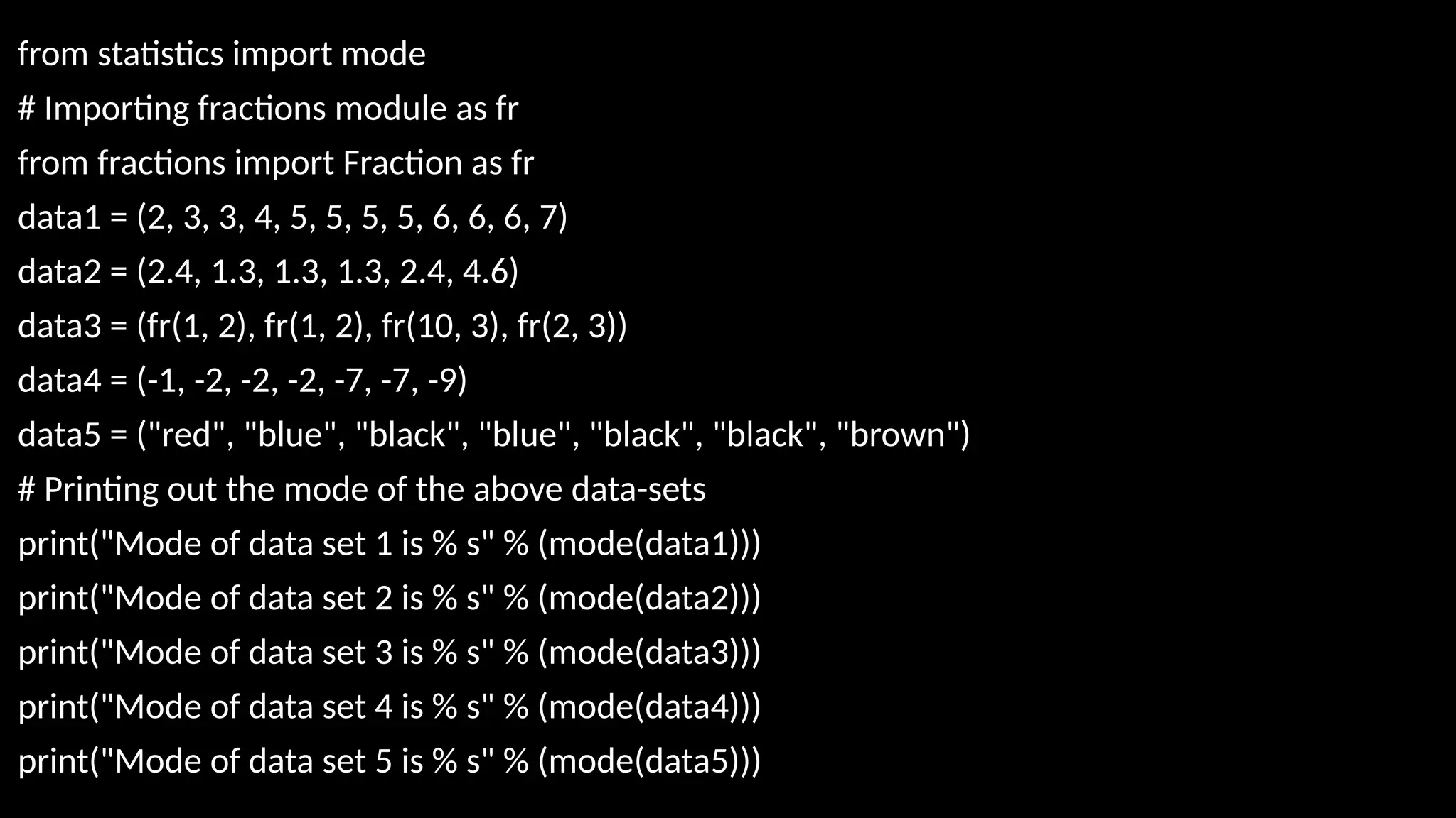
8. from statistics import mode
# Importing fractions module as fr
from fractions import Fraction as fr
data1 = (2, 3, 3, 4, 5, 5, 5, 5, 6, 6, 6, 7)
data2 = (2.4, 1.3, 1.3, 1.3, 2.4, 4.6)
data3 = (fr(1, 2), fr(1, 2), fr(10, 3), fr(2, 3))
data4 = (-1, -2, -2, -2, -7, -7, -9)
data5 = ("red", "blue", "black", "blue", "black", "black", "brown")
# Printing out the mode of the above data-sets
print("Mode of data set 1 is % s" % (mode(data1)))
print("Mode of data set 2 is % s" % (mode(data2)))
print("Mode of data set 3 is % s" % (mode(data3)))
print("Mode of data set 4 is % s" % (mode(data4)))
print("Mode of data set 5 is % s" % (mode(data5)))

9. The measure of variability is known as the spread of data or how well our data is distributed.
The most common variability measures are:
Range,Variance,Standard deviation
Range
The difference between the largest and smallest data point in our data set is known as the
range.
Range = Largest data value – smallest data value
arr = [1, 2, 3, 4, 5]
Maximum = max(arr)
# Finding Min
Minimum = min(arr)
# Difference Of Max and Min
Range = Maximum-Minimum
print("Maximum = {}, Minimum = {} and Range = {}".format(
Maximum, Minimum, Range))

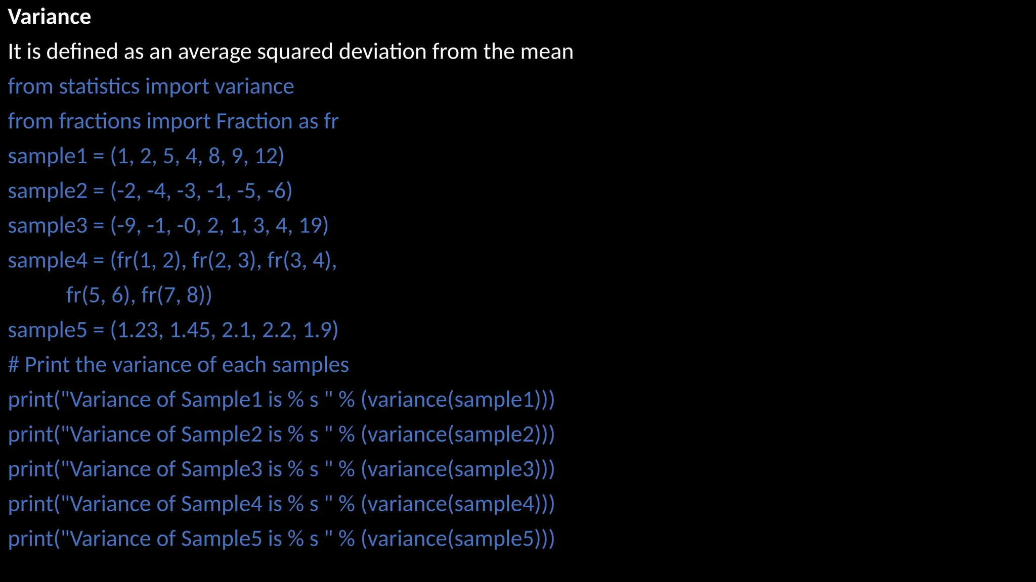
10. Variance
It is defined as an average squared deviation from the mean
from statistics import variance
from fractions import Fraction as fr
sample1 = (1, 2, 5, 4, 8, 9, 12)
sample2 = (-2, -4, -3, -1, -5, -6)
sample3 = (-9, -1, -0, 2, 1, 3, 4, 19)
sample4 = (fr(1, 2), fr(2, 3), fr(3, 4),
fr(5, 6), fr(7, 8))
sample5 = (1.23, 1.45, 2.1, 2.2, 1.9)
# Print the variance of each samples
print("Variance of Sample1 is % s " % (variance(sample1)))
print("Variance of Sample2 is % s " % (variance(sample2)))
print("Variance of Sample3 is % s " % (variance(sample3)))
print("Variance of Sample4 is % s " % (variance(sample4)))
print("Variance of Sample5 is % s " % (variance(sample5)))

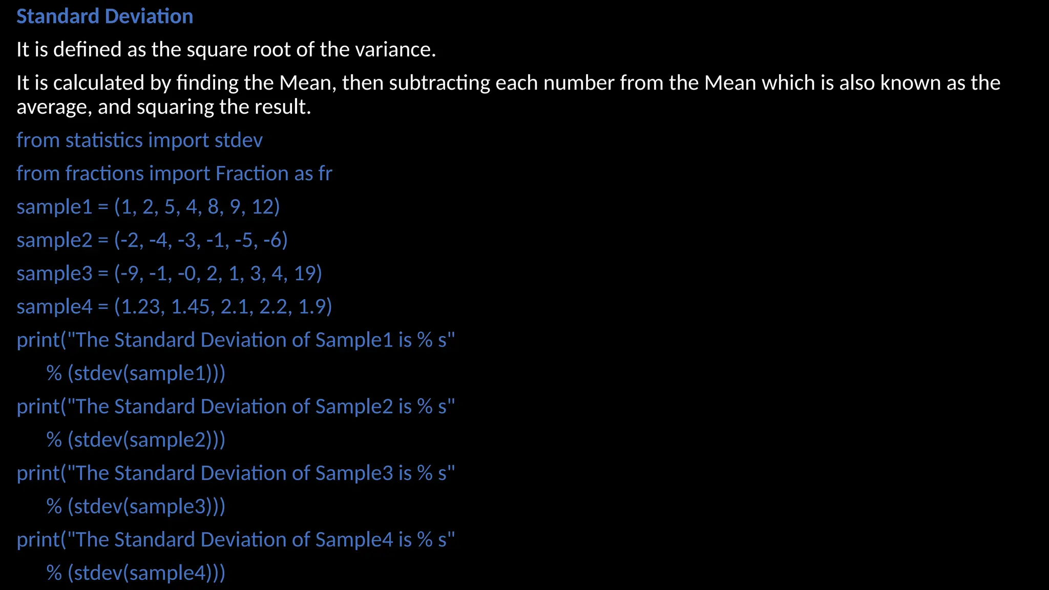
11. Standard Deviation
It is defined as the square root of the variance.
It is calculated by finding the Mean, then subtracting each number from the Mean which is also known as the
average, and squaring the result.
from statistics import stdev
from fractions import Fraction as fr
sample1 = (1, 2, 5, 4, 8, 9, 12)
sample2 = (-2, -4, -3, -1, -5, -6)
sample3 = (-9, -1, -0, 2, 1, 3, 4, 19)
sample4 = (1.23, 1.45, 2.1, 2.2, 1.9)
print("The Standard Deviation of Sample1 is % s"
% (stdev(sample1)))
print("The Standard Deviation of Sample2 is % s"
% (stdev(sample2)))
print("The Standard Deviation of Sample3 is % s"
% (stdev(sample3)))
print("The Standard Deviation of Sample4 is % s"
% (stdev(sample4)))

12. import numpy as np
import pandas as pd
from scipy import stats
#Load Example dataset
data = [10, 12, 9, 15, 14, 13, 12, 11, 10, 15]
# Or with pandas DataFrame
df = pd.DataFrame({
'Scores': [10, 12, 9, 15, 14, 13, 12, 11, 10, 15]
})
#Descriptive Statistics
# Mean, Median, Standard Deviation
mean_val = np.mean(data)
median_val = np.median(data)
std_val = np.std(data, ddof=1) # ddof=1 for sample std
print("Mean:", mean_val)
print("Median:", median_val)
print("Standard Deviation:", std_val)
# Using pandas (quicker)
print(df['Scores'].describe()) # count, mean, std, min, quartiles, max

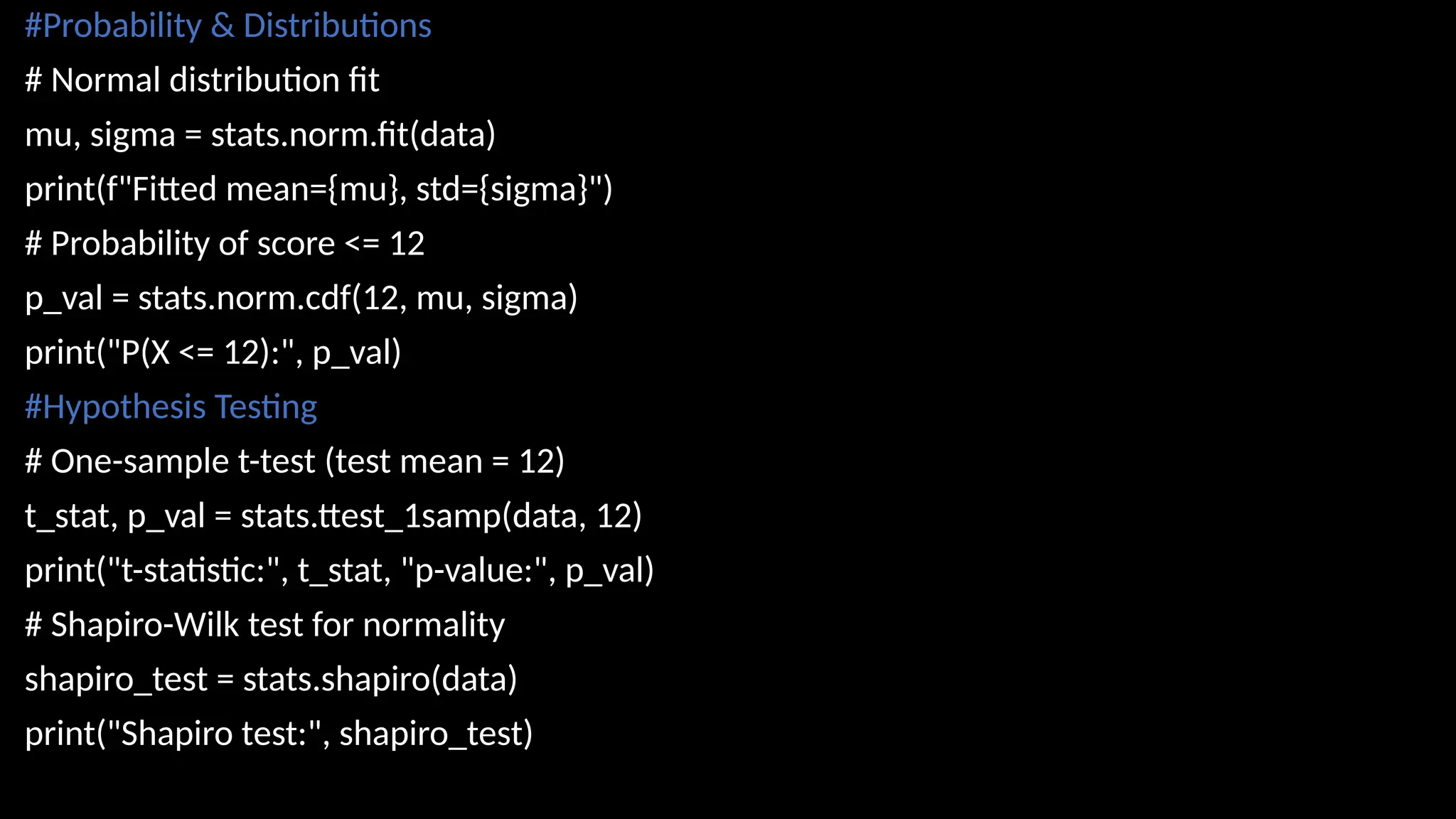
13. #Probability & Distributions
# Normal distribution fit
mu, sigma = stats.norm.fit(data)
print(f"Fitted mean={mu}, std={sigma}")
# Probability of score <= 12
p_val = stats.norm.cdf(12, mu, sigma)
print("P(X <= 12):", p_val)
#Hypothesis Testing
# One-sample t-test (test mean = 12)
t_stat, p_val = stats.ttest_1samp(data, 12)
print("t-statistic:", t_stat, "p-value:", p_val)
# Shapiro-Wilk test for normality
shapiro_test = stats.shapiro(data)
print("Shapiro test:", shapiro_test)

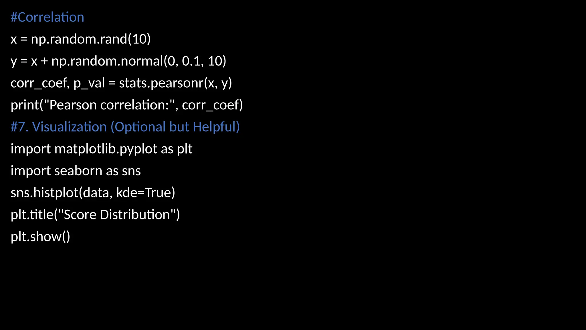
14. #Correlation
x = np.random.rand(10)
y = x + np.random.normal(0, 0.1, 10)
corr_coef, p_val = stats.pearsonr(x, y)
print("Pearson correlation:", corr_coef)
#7. Visualization (Optional but Helpful)
import matplotlib.pyplot as plt
import seaborn as sns
sns.histplot(data, kde=True)
plt.title("Score Distribution")
plt.show()

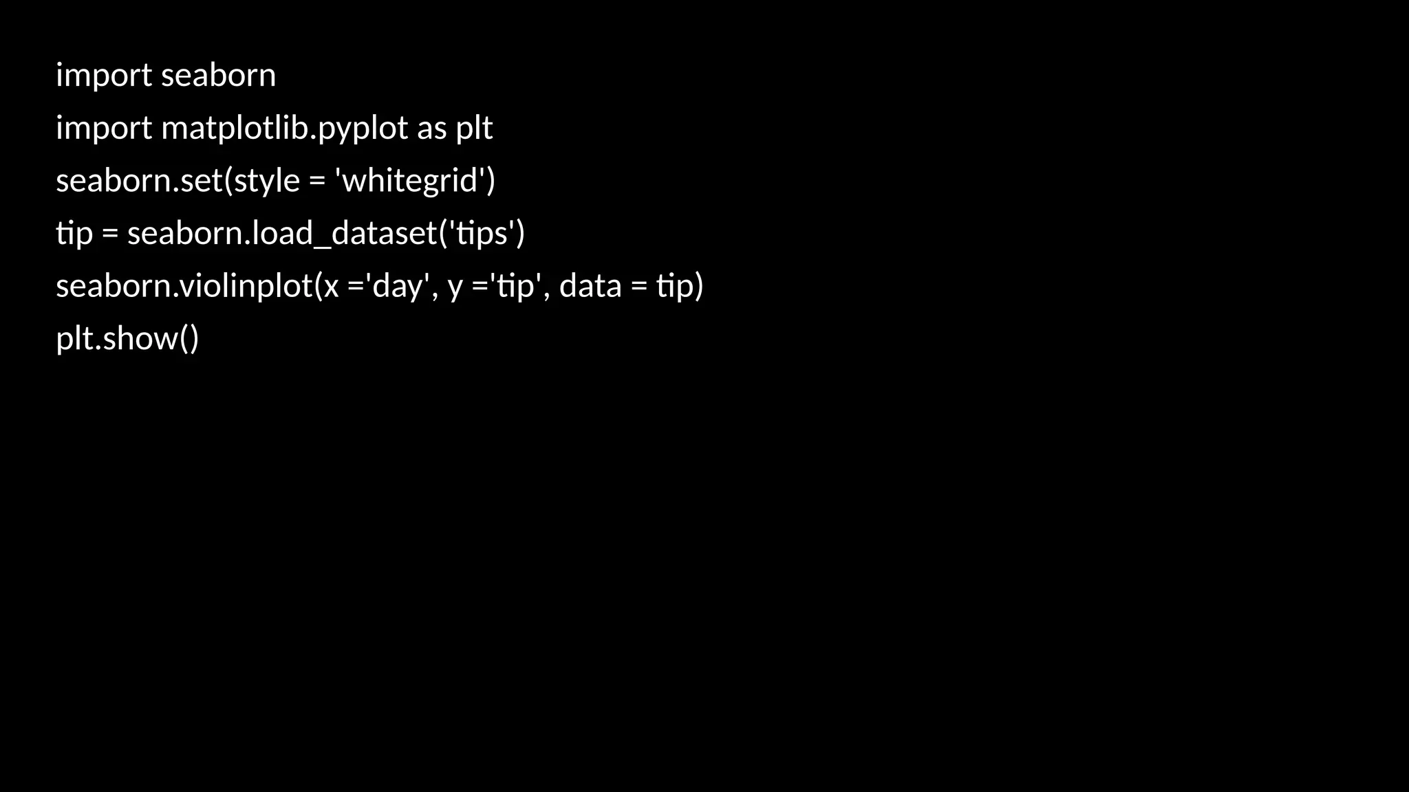
15. import seaborn
import matplotlib.pyplot as plt
seaborn.set(style = 'whitegrid')
tip = seaborn.load_dataset('tips')
seaborn.violinplot(x ='day', y ='tip', data = tip)
plt.show()

16. Stripped plots:
# Stripplot using inbuilt data-set
import matplotlib.pyplot as plt
import seaborn as sns
sns.set(style="whitegrid")
# loading data-set
iris = sns.load_dataset('iris')
# plotting strip plot with seaborn
# deciding the attributes of dataset on
# which plot should be made
ax = sns.stripplot(x='species', y='sepal_length', data=iris)
# giving title to the plot
plt.title('Graph')
# function to show plot
plt.show()

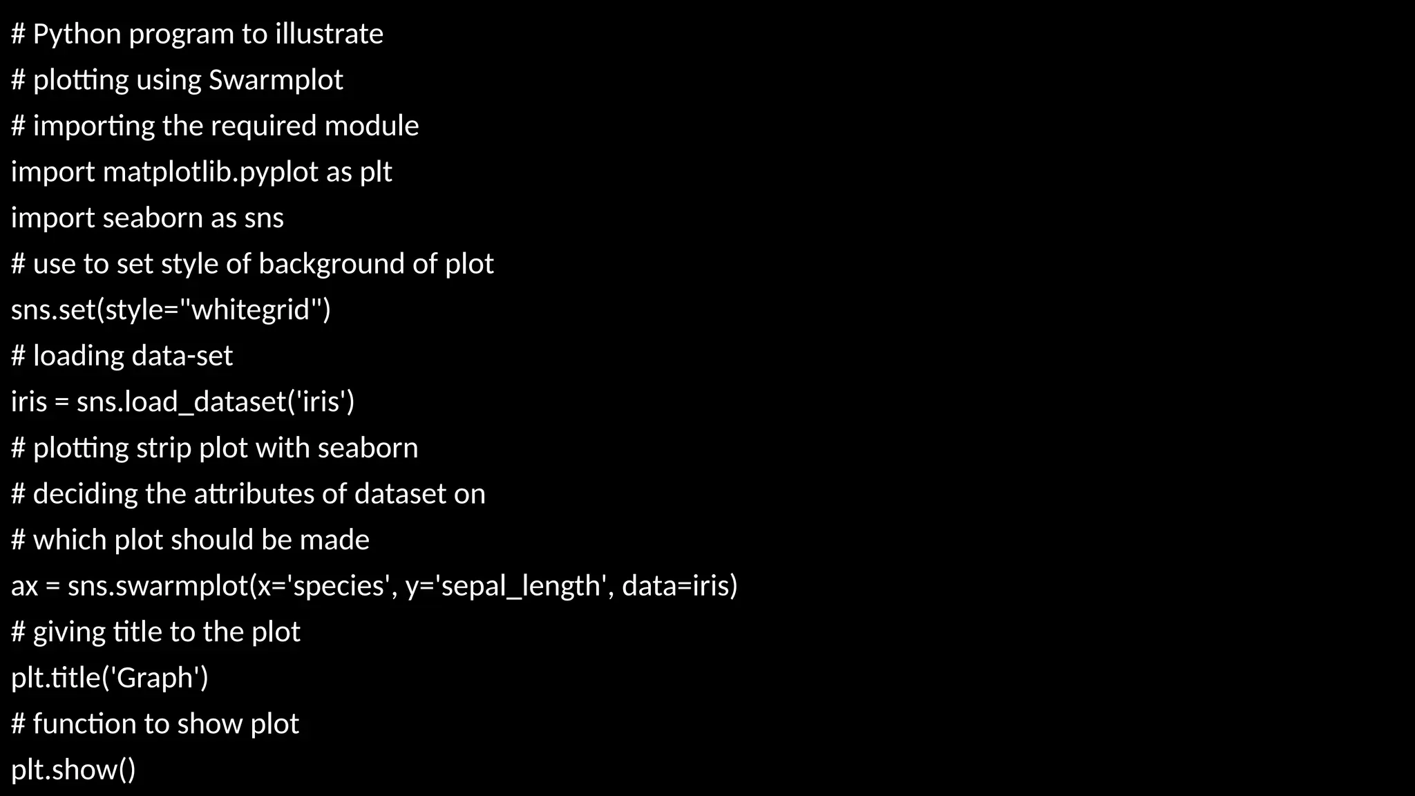
17. # Python program to illustrate
# plotting using Swarmplot
# importing the required module
import matplotlib.pyplot as plt
import seaborn as sns
# use to set style of background of plot
sns.set(style="whitegrid")
# loading data-set
iris = sns.load_dataset('iris')
# plotting strip plot with seaborn
# deciding the attributes of dataset on
# which plot should be made
ax = sns.swarmplot(x='species', y='sepal_length', data=iris)
# giving title to the plot
plt.title('Graph')
# function to show plot
plt.show()