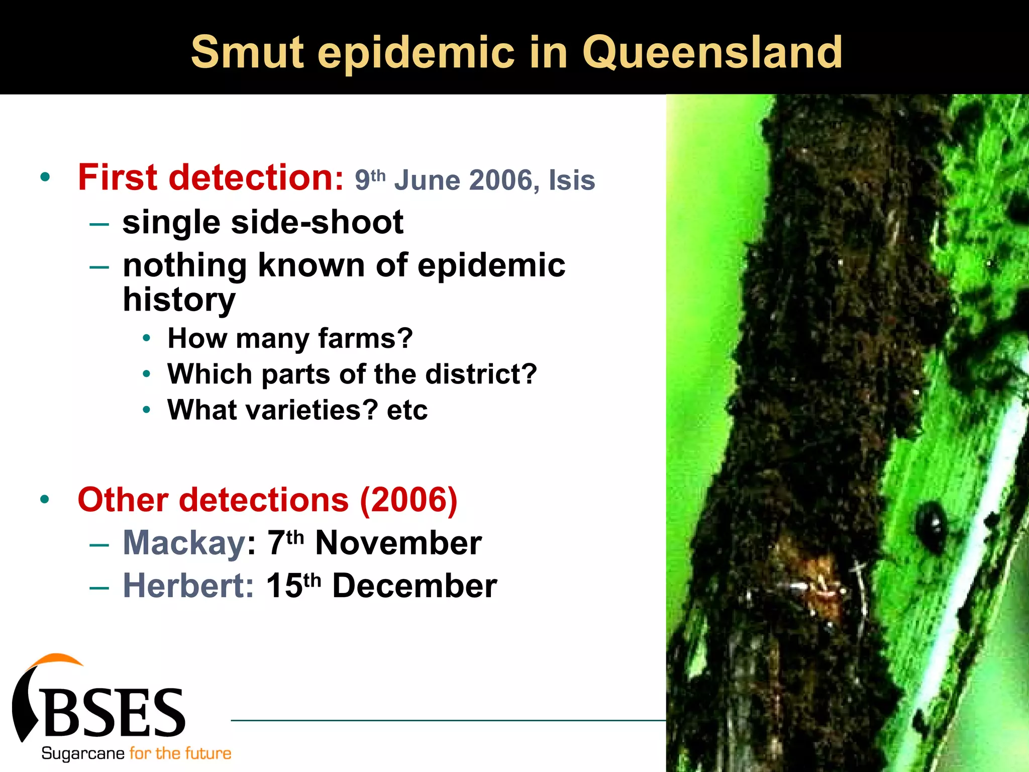
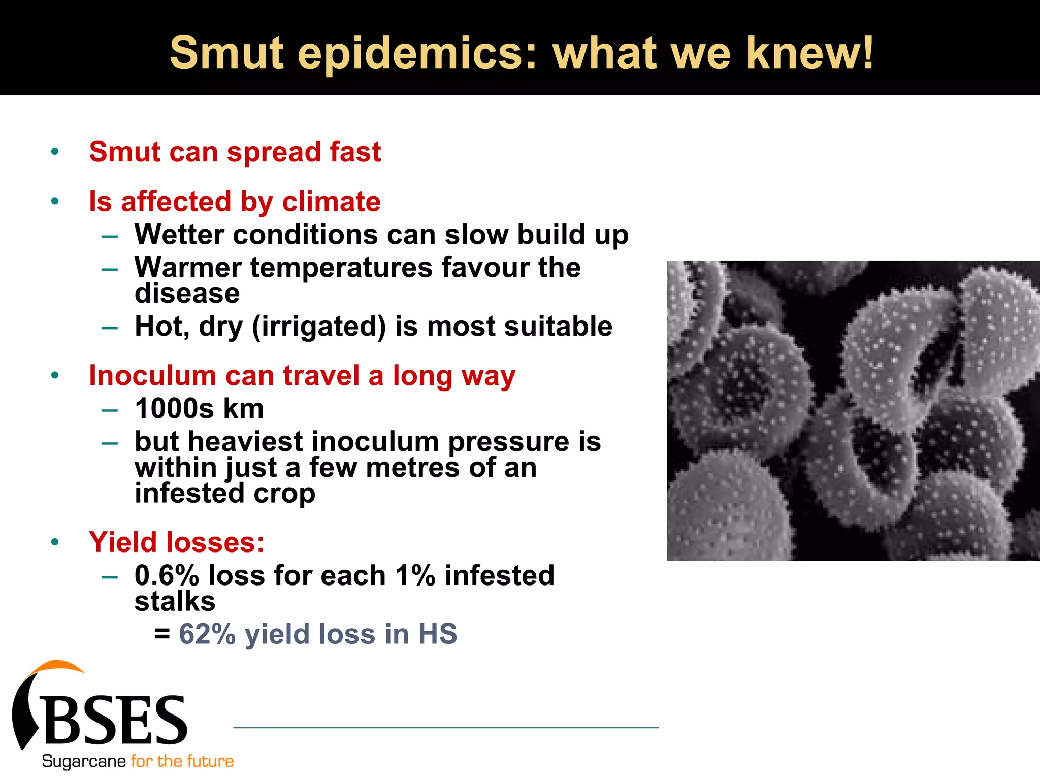
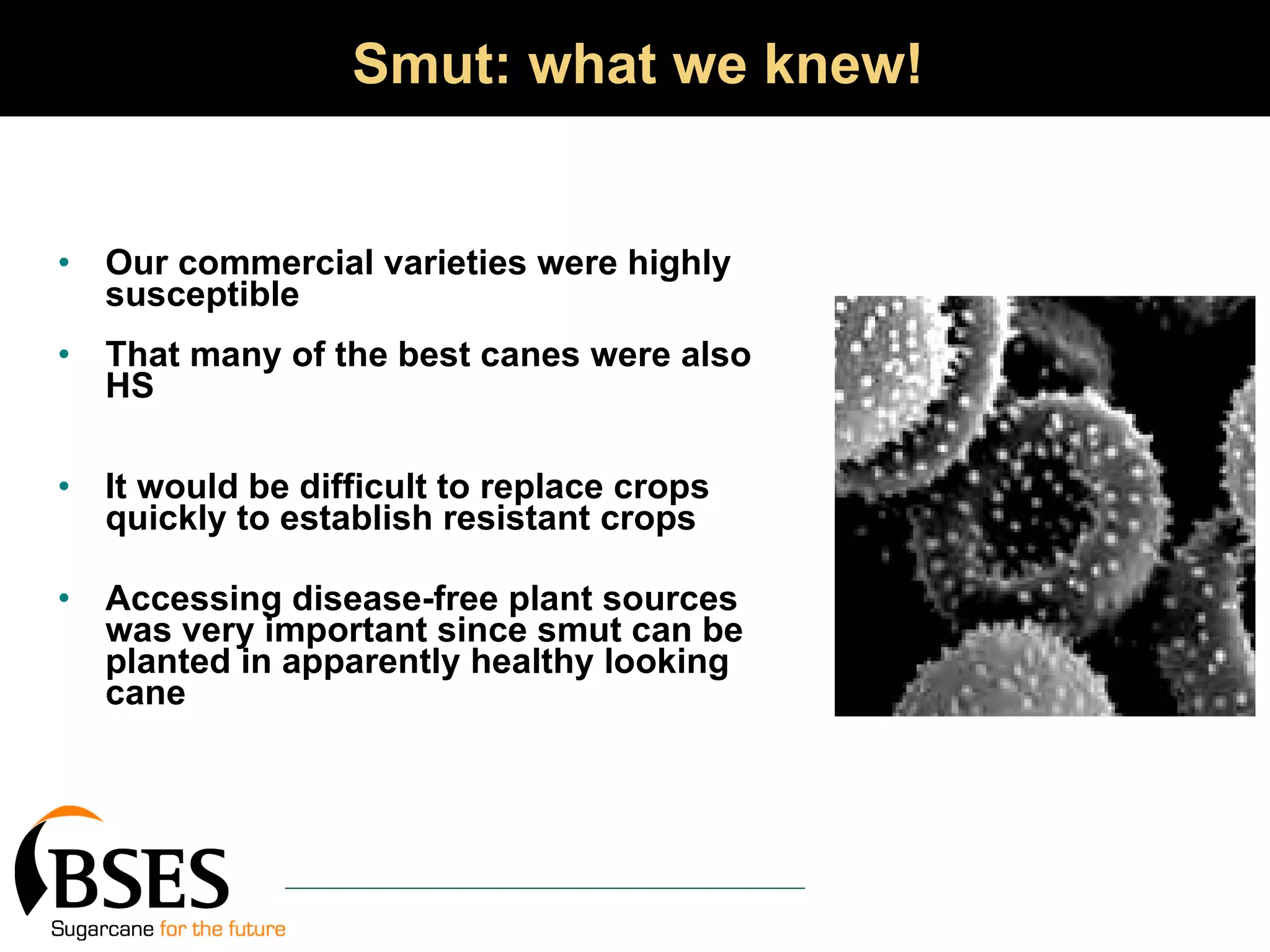
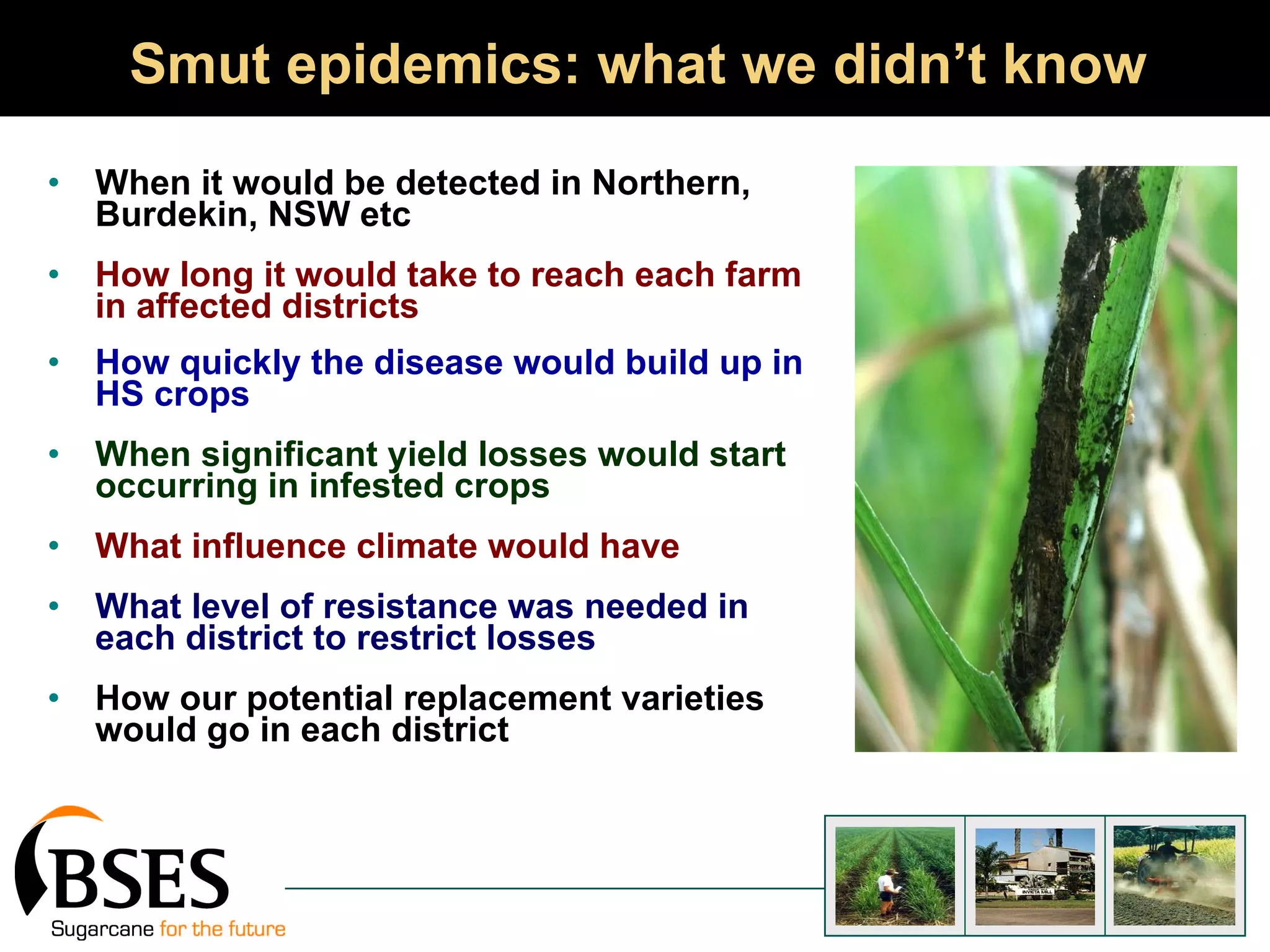
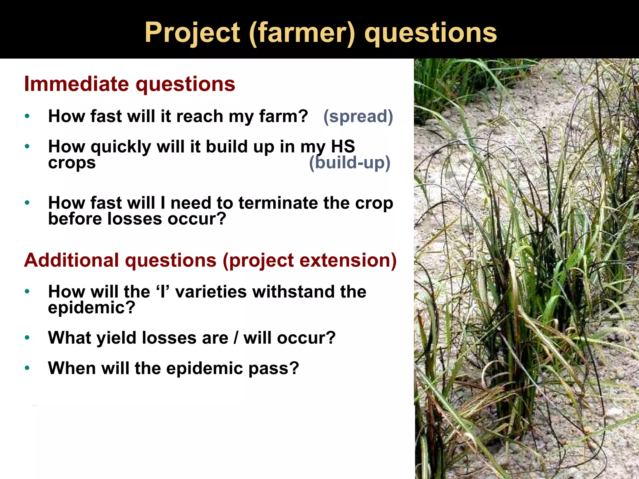
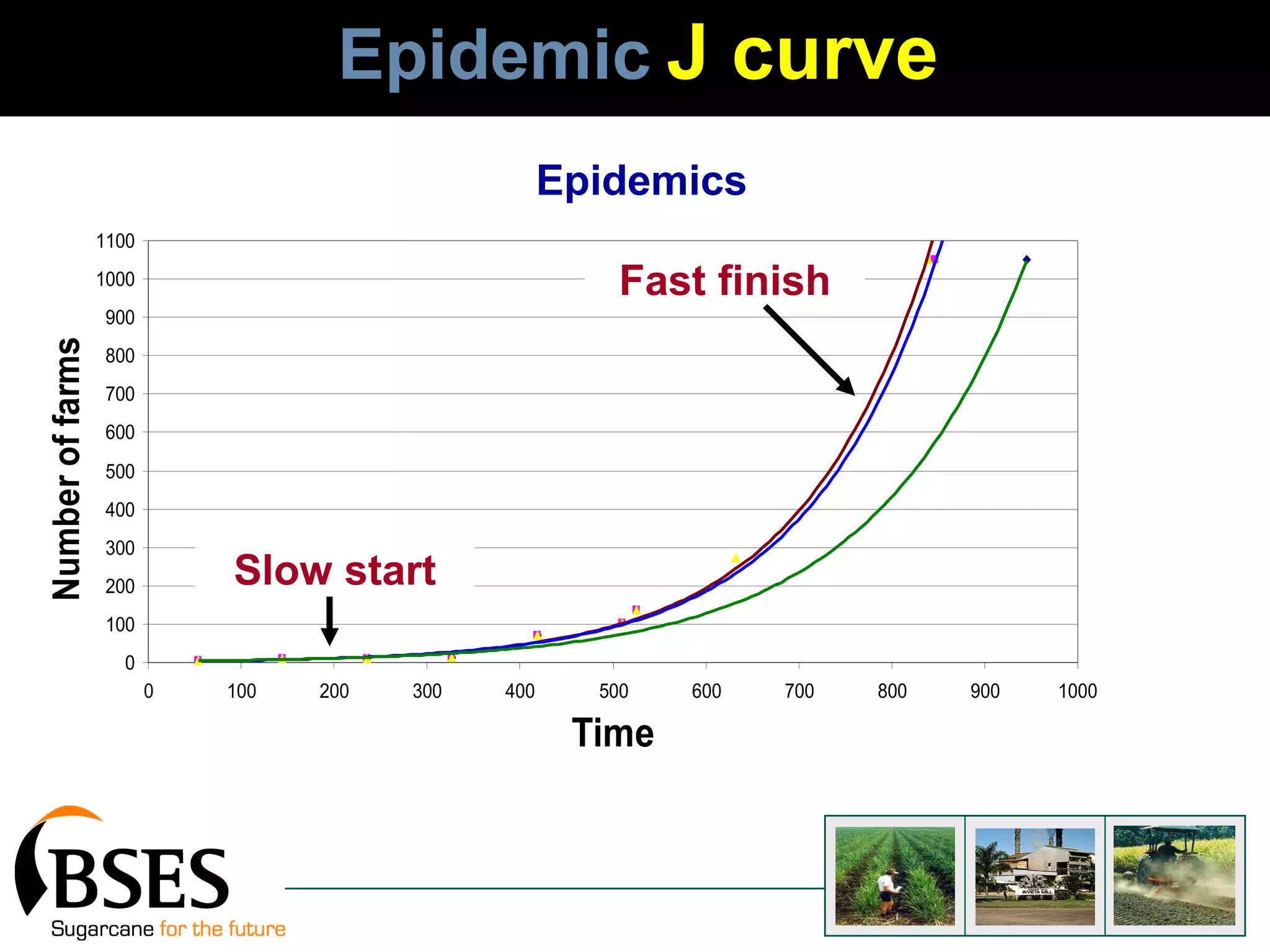
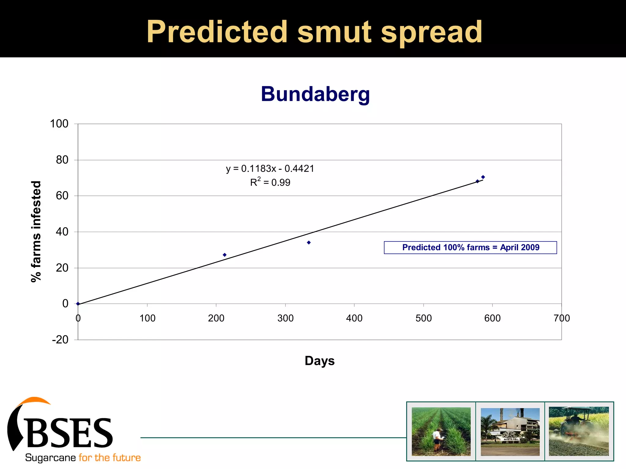
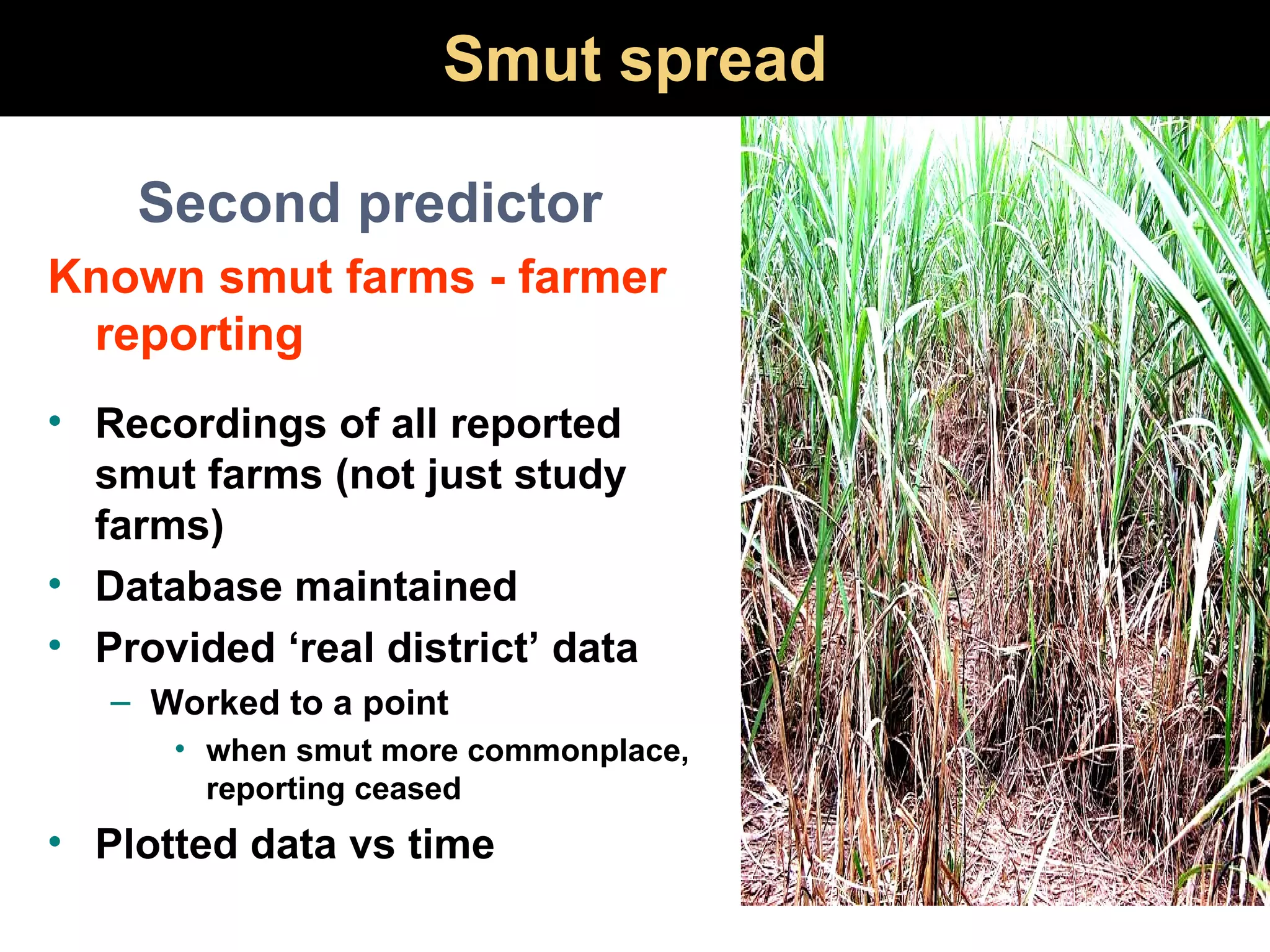
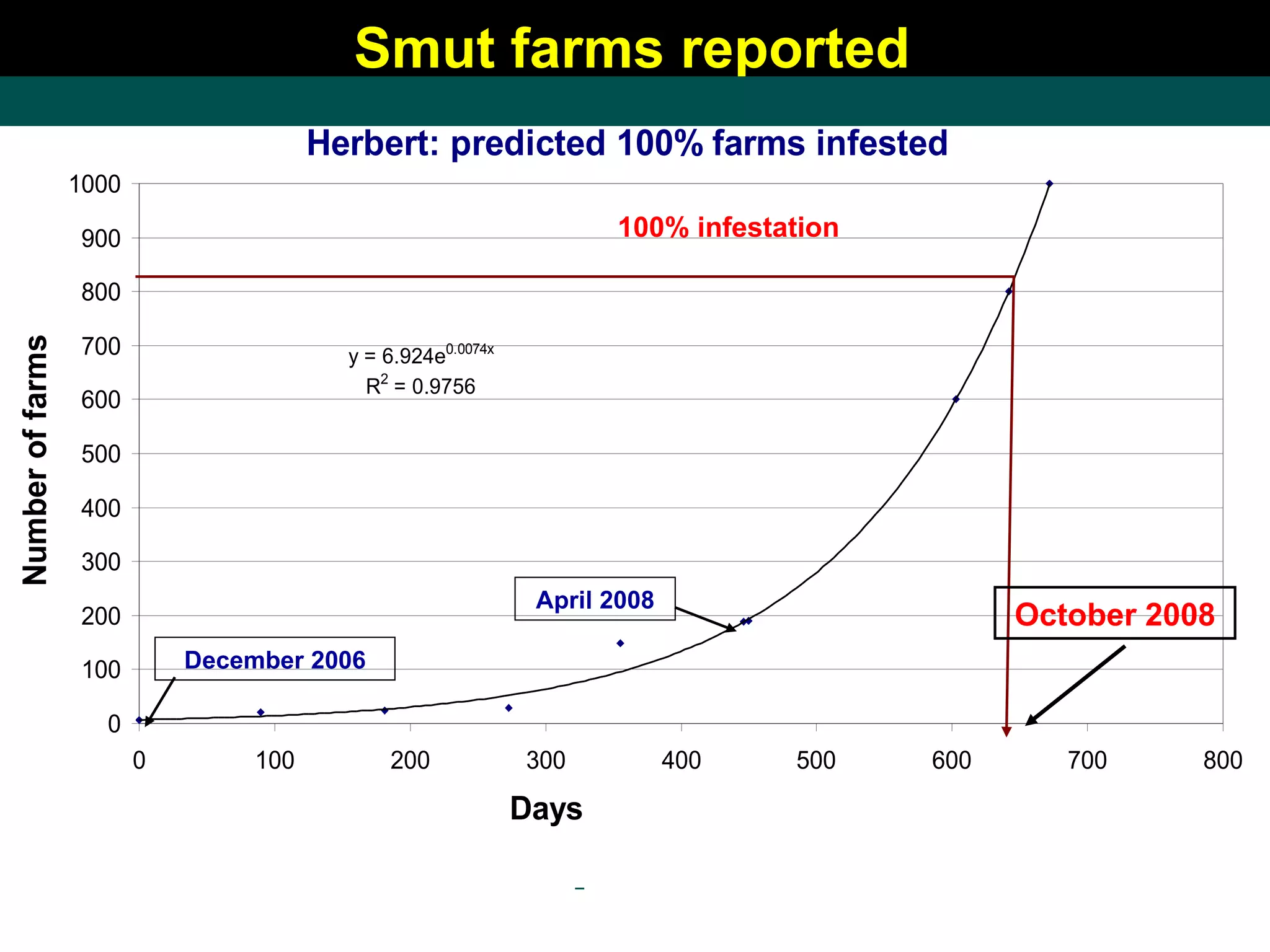
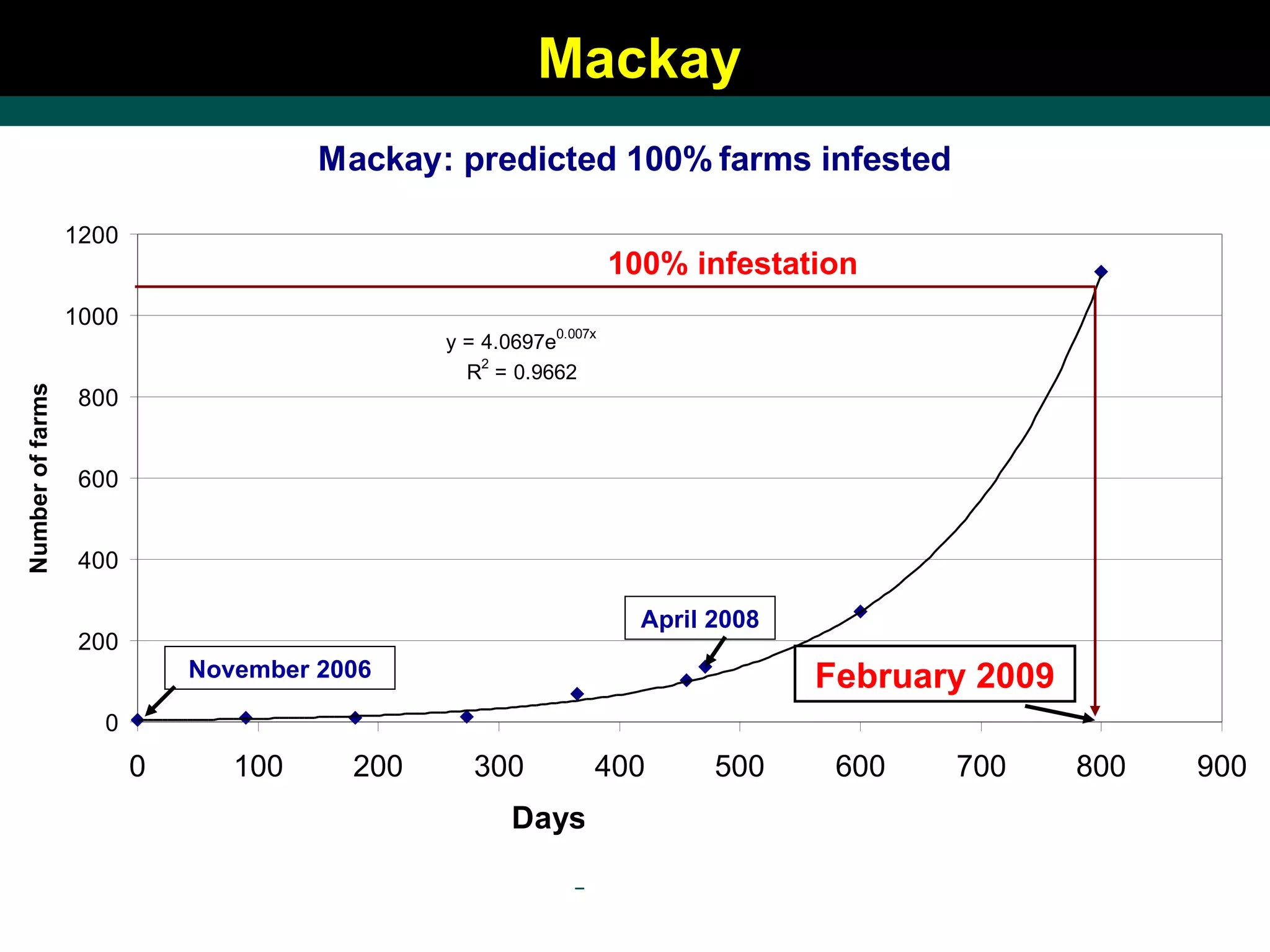
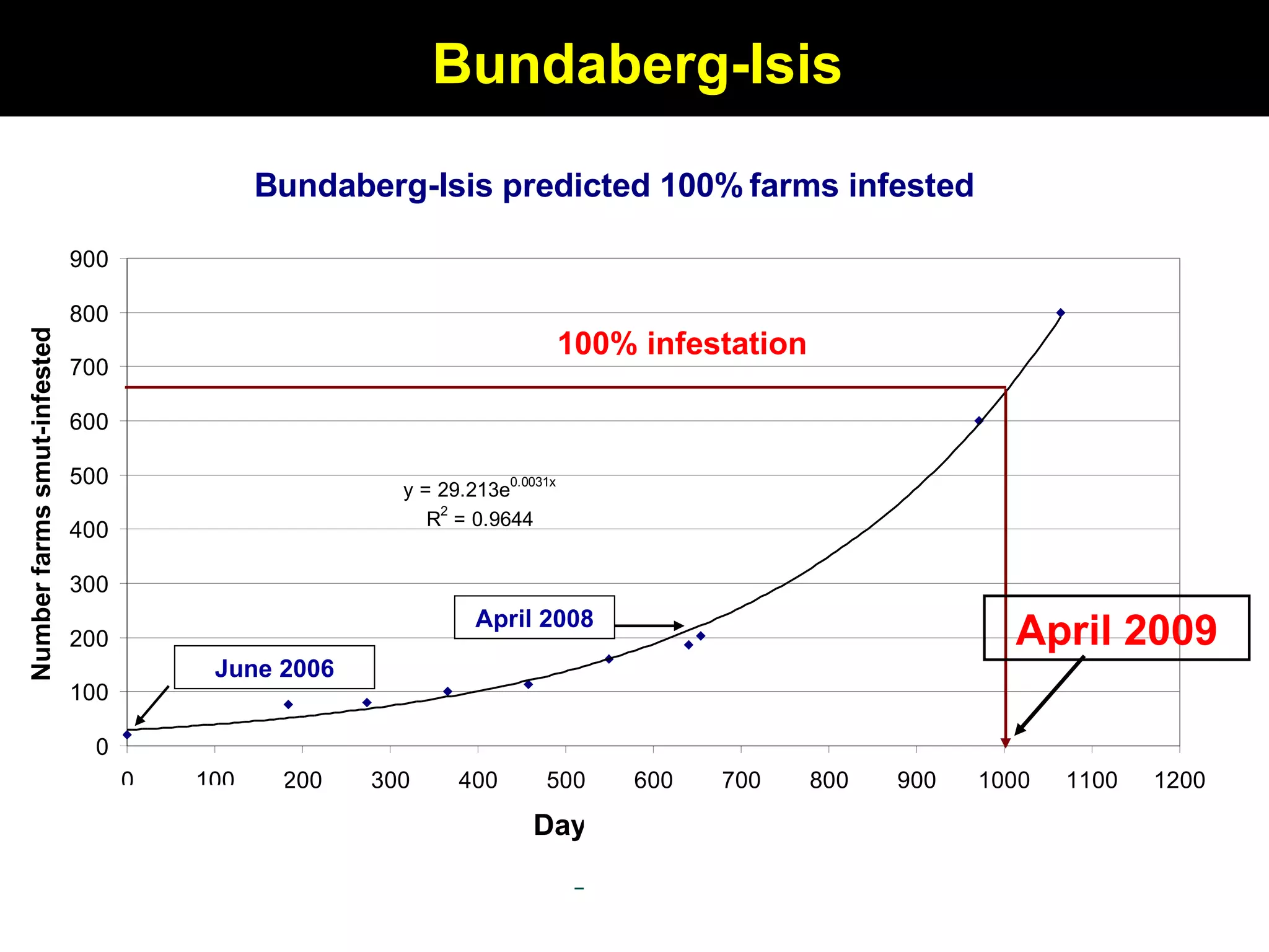
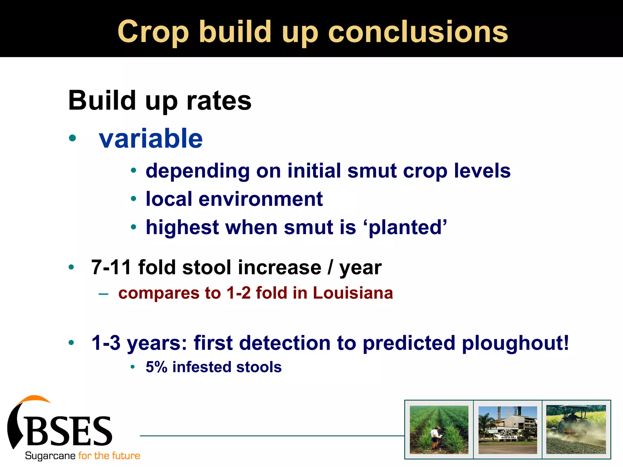
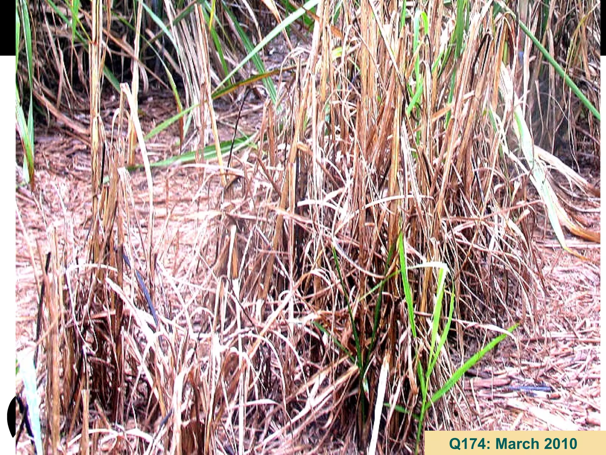
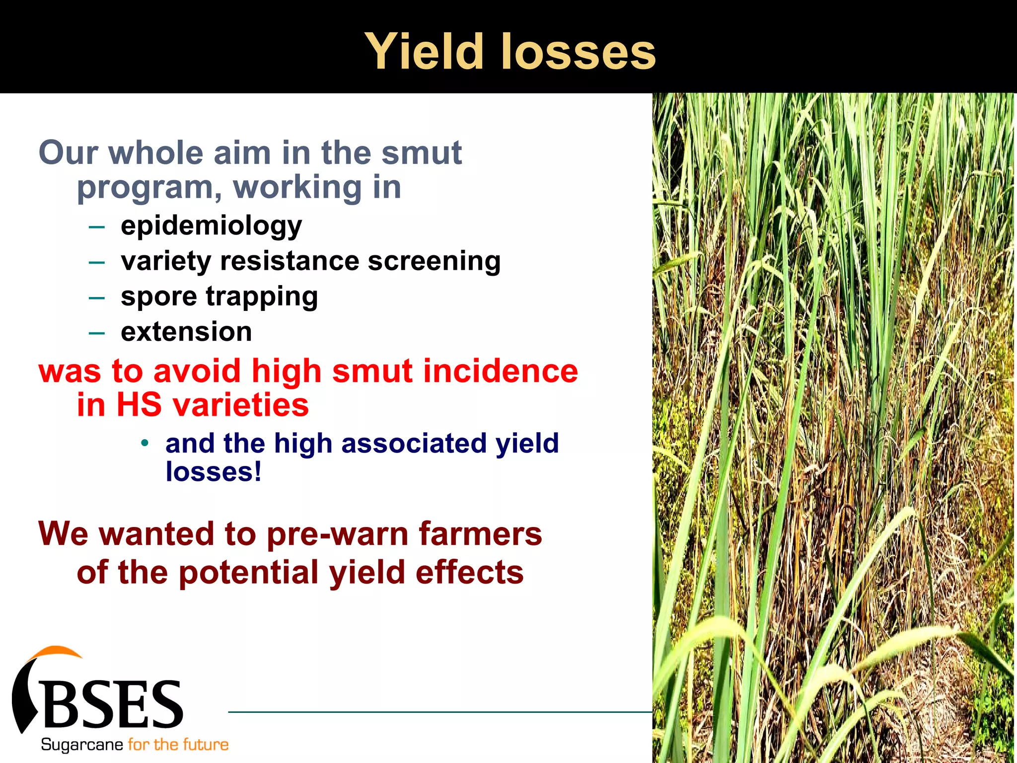
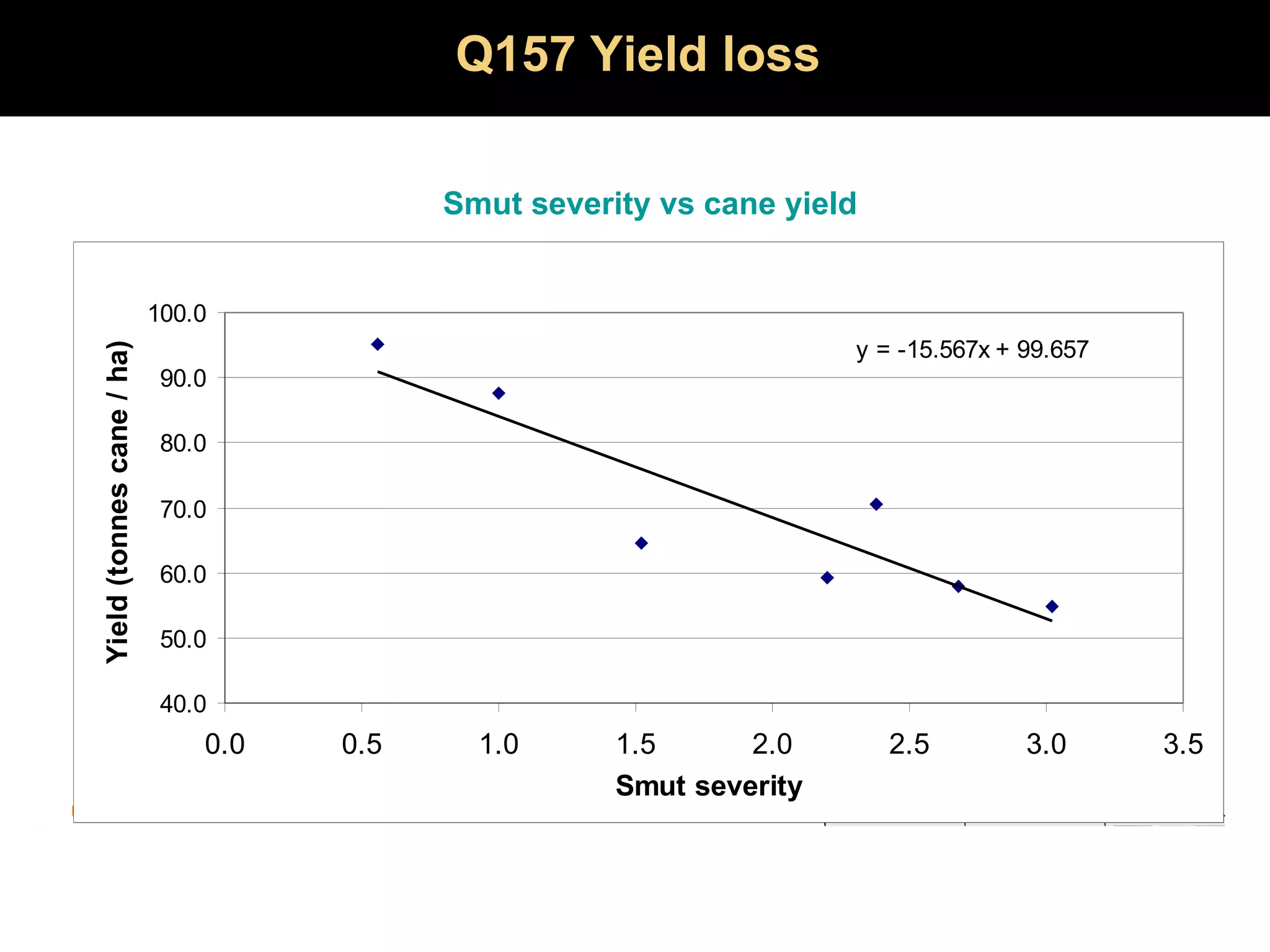
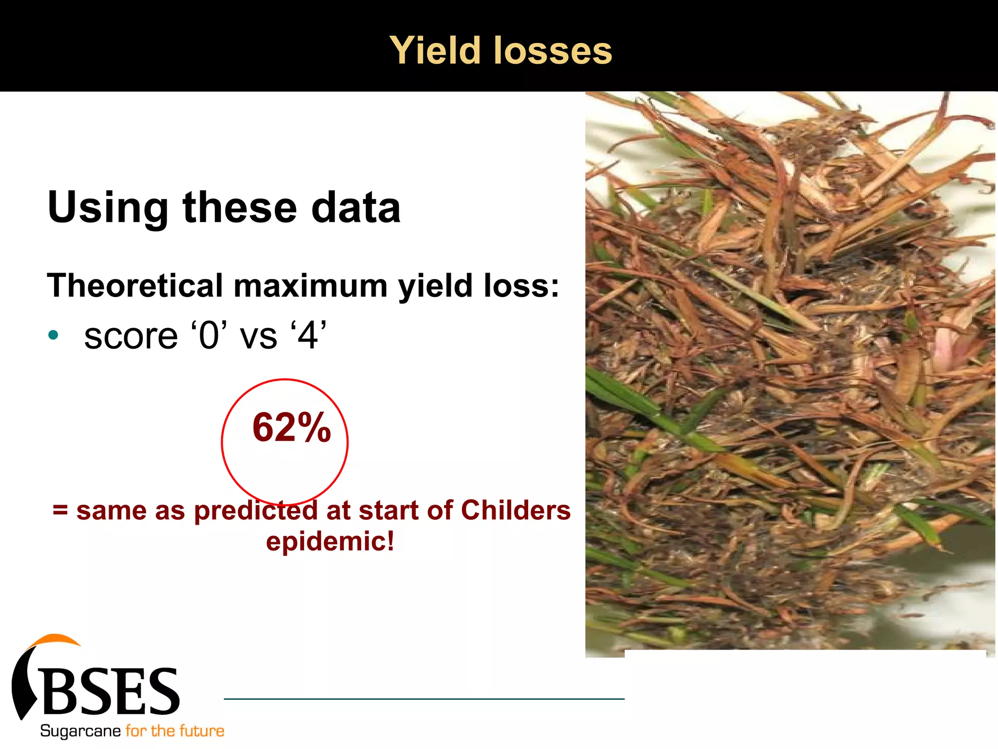
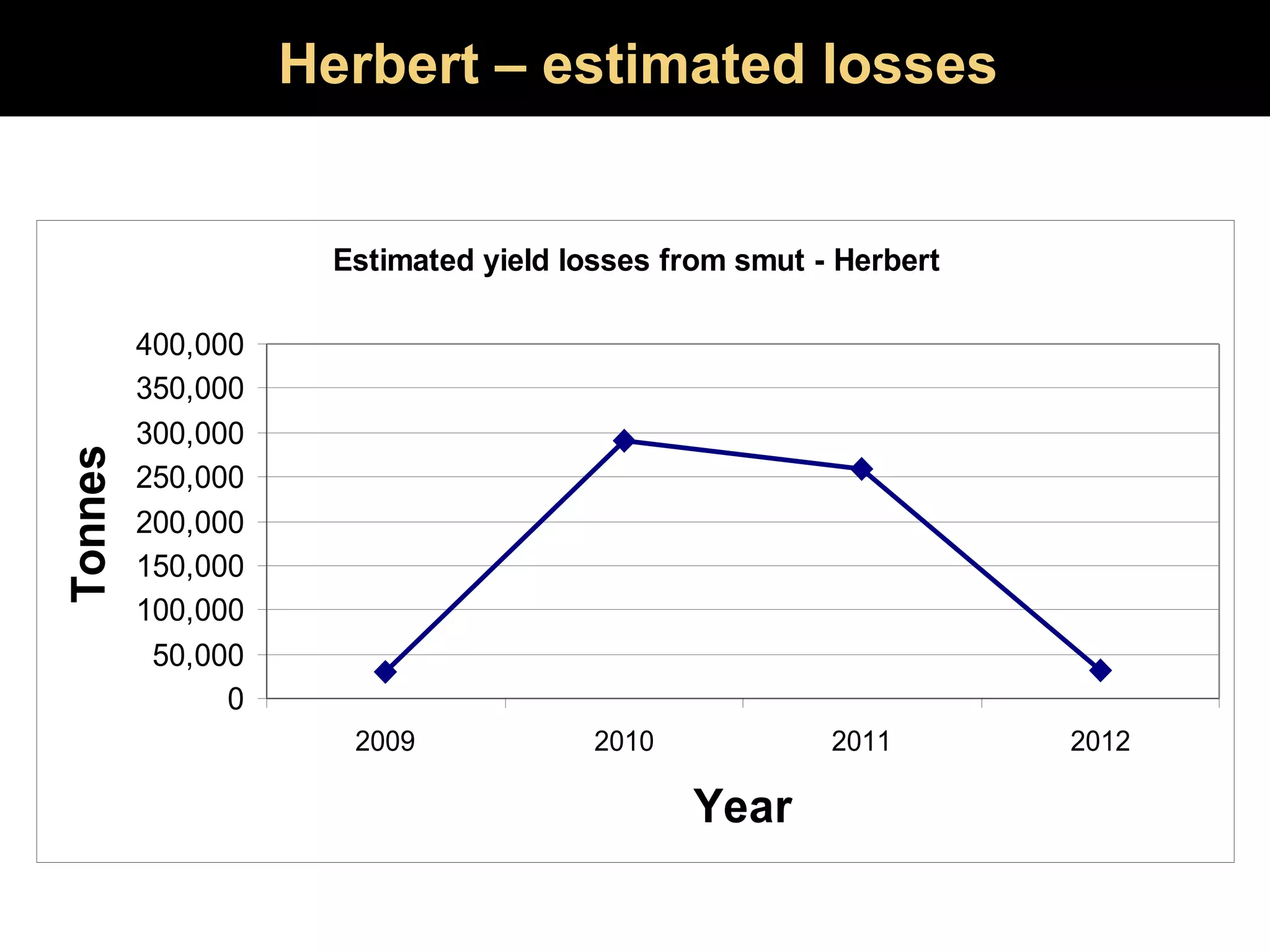
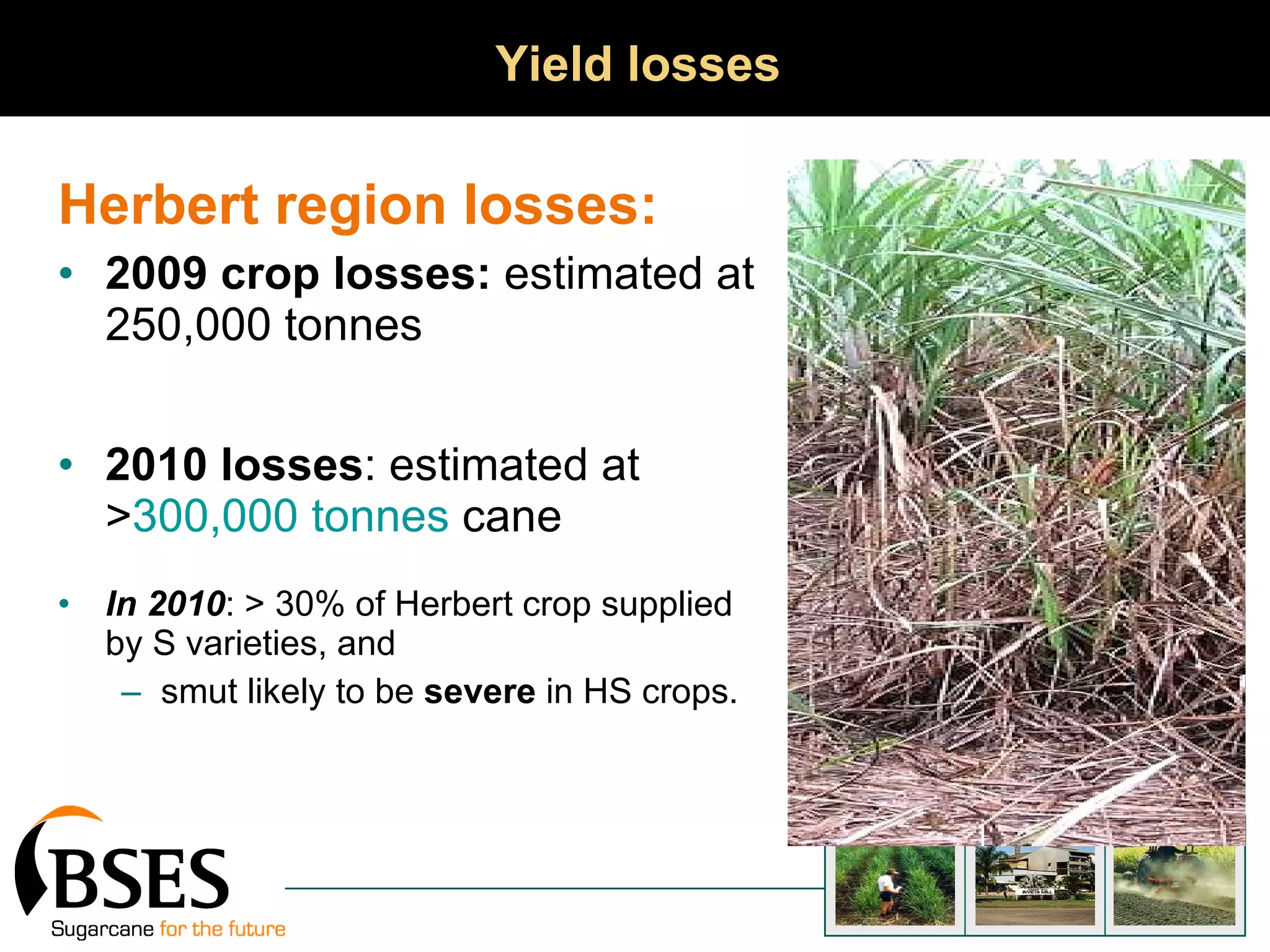
SMUT EPIDEMIOLOGY   SRDC-funded project Rob Magarey BSES Limited, Tully
Epidemiology  Definition Study of the spread, build up and effect of an epidemic
Smut epidemic in Queensland First detection :  9 th  June 2006, Isis single side-shoot nothing known of epidemic history How many farms? Which parts of the district? What varieties? etc Other detections (2006) Mackay : 7 th  November  Herbert:  15 th  December
Smut epidemics: what we knew! Smut can spread fast Is affected by climate Wetter conditions can slow build up Warmer temperatures favour the disease Hot, dry (irrigated) is most suitable Inoculum can travel a long way 1000s km but heaviest inoculum pressure is within just a few metres of an infested crop  Yield losses:  0.6% loss for each 1% infested stalks  =  62% yield loss in HS
Smut: what we knew! Our commercial varieties were highly susceptible That many of the best canes were also HS It would be difficult to replace crops quickly to establish resistant crops Accessing disease-free plant sources was very important since smut can be planted in apparently healthy looking cane
Smut epidemics: what we didn’t know When it would be detected in Northern, Burdekin, NSW etc How long it would take to reach each farm in affected districts How quickly the disease would build up in HS crops When significant yield losses would start occurring in infested crops What influence climate would have What level of resistance was needed in each district to restrict losses How our potential replacement varieties would go in each district
Project (farmer) questions Immediate questions How fast will it reach my farm?  (spread) How quickly will it build up in my HS crops    (build-up) How fast will I need to terminate the crop before losses occur? Additional questions (project extension) How will the ‘I’ varieties withstand the epidemic? What yield losses are / will occur? When will the epidemic pass?
Epidemic   J curve Slow start Fast finish Epidemics
Epidemiology methods Two initial focus areas Smut  spread  Monitoring a non-diseased farm network Smut  build up   increase in % stools in example susceptible crops
Smut spread
Smut spread Two strategies Smut-free farm network Farmer reporting Smut-free network Un-infested farms were selected Networks in each of Bundaberg, Mackay, Herbert Inspected regularly for smut Speed of spread monitored
Predicted smut spread Bundaberg
Smut spread Second predictor Known smut farms - farmer reporting Recordings of all reported smut farms (not just study farms) Database maintained Provided ‘real district’ data Worked to a point when smut more commonplace, reporting ceased Plotted data vs time
Smut farms reported   December 2006 April 2008 100% infestation October 2008
Mackay November 2006 April 2008 February 2009 100% infestation
Bundaberg-Isis 100% infestation April 2009 April 2008 June 2006


Smut build-up
Smut build up ‘in-crop’ Example HS crops selected Individual stools monitored (+ or – smut) Data recorded using GPS Stools mapped Increase in smut calculated Escalation rates determined
Q205 Bundaberg
Q205 Bundaberg
Q205 Bundaberg
Q205 Bundaberg
Q205 Bundaberg
Q205 Bundaberg
Crop build up conclusions Build up rates variable depending on initial smut crop levels local environment highest when smut is ‘planted’ 7-11 fold stool increase / year compares to 1-2 fold in Louisiana 1-3 years: first detection to predicted ploughout! 5% infested stools
Smut yield losses
Q174: March 2010
Yield losses Our whole aim in the smut program, working in epidemiology variety resistance screening spore trapping extension was to avoid high smut incidence in HS varieties and the high associated yield losses! We wanted to pre-warn farmers of the potential yield effects
Quantifying losses Strategy:  choose 7 plots in a crop with varying smut levels Assess yield in each plot Relate smut severity to yield Identified a badly-affected 2009 crop in the Herbert (Abergowrie) Highly susceptible Q157
Yield losses Selected 7 plots :  2 rows x 7m applied smut severity scores to all stools  0  = no smut 1  = a few primary whips only 2  = moderate number of whips but no grassiness 3  = 50-75% primary whips and some grassiness 4  = >75% primary whips and most of the stool grassy Calculated average severity / plot Cut / weighed all cane in plots quantified weight cane / plot Graphed yield vs severity
Q157 Yield loss Smut severity vs cane yield
Yield losses Using these data   Theoretical maximum yield loss: score ‘0’ vs ‘4’  62% = same as predicted at start of Childers epidemic!
Yield losses What losses did the farmer suffer in that crop (whole crop)? Depends on average crop severity Selected 20 plots scattered randomly through the crop (10m length) Scored all stools in all plots Found average severity = average whole crop severity Related yield loss estimate x severity to estimate total crop losses in that particular crop
Average severity across whole crop 20 plots  Mean severity score  =  1.6  (0 to 4 severity scale) Related to yield   using the previous graph The average smut-induced yield loss for that whole crop  =  26%. Yield losses
Variety effects Field
Strong field variety effects Herbert Variety # crops Variety # crops Q158 154 Q220 3 Q174 151 Q233 3 Q157 67 Q115 3 Q204 18 Q152 3 Q186 14 Q164 3 Q194 14 Q216 3 Q162 13 Q172 2 Q166 10 Q127 2 Q195 10 Q138 2 Q200 5 Q99 1 Argos 5 KQ228 1 Q179 5 Q219 1 Q190 3 Q183 1
What level of resistance is needed? Natural spread trial planted in Mackay Varieties varying in resistance  Included important ‘replacement’ canes Planted ‘clean’ Monitored disease buildup vs HS canes Worst affected farm in Mackay
Mackay natural spread – April 2009
Highly susceptible canes   Severe smut very quickly Disaster! Susceptible (7-8) Not so fast Intermediate canes pretty good especially Q183, Q135, Q208 Resistant canes No problem Field resistance
Q208: a major variety! Some have expressed concern about disease levels In Mackay – some significant disease (around 1.5% disease) Herbert – one report of 9% infested stools But following crops have had low smut levels this also seen in the Ord   No problem with this variety!
When will the epidemic pass? Epidemic modelling
Epidemic modelling Based on weighted parameter % S, I and R crops: district x year plus estimated smut severity  Calculated parameter: ‘relative smut’  - smut indicator  Models: guide to when the maximum smut stress on ‘I’ varieties
Herbert district
Epidemic modelling RISE   of the epidemic principally about smut spread escalation  in HS crops (plenty around) FALL   of the epidemic almost wholly to do with: - elimination of HS crops
Bundaberg-Childers
Epidemic modelling Bundaberg-Childers Similar pattern to the Herbert Peak in 2009 (a little earlier) More rapid replacement of susceptibles Peak smaller than Herbert
Smut comparison x district
Herbert – estimated losses
Yield losses Herbert region losses:   2009 crop losses:  estimated at 250,000 tonnes 2010 losses : estimated at  > 300,000 tonnes  cane In 2010 : > 30% of Herbert crop supplied by S varieties, and  smut likely to be  severe  in HS crops.
Important management points Maintain transition to resistant varieties   if too slow, there will be high direct losses, and  maximum inoculum pressure on intermediates Industry needs to make common sense decisions on which crops to terminate
Conclusions This is ‘crunch’ time - yield loss phase Losses will be significant in Herbert, Mackay and Bundaberg in 2010 and 2011 Largely confined to the HS varieties Urgent need to transition out of HS to avoid yield losses!
Overall conclusions Smut: 2-3 years to spread to all farms in district Significant losses: within 3 years from first finding of smut in a crop (susceptible) 10-fold stool increase each year Some intermediates will be OK Smut losses: a little slower to occur than anticipated

SRDC seminar

  • 1.
    SMUT EPIDEMIOLOGY SRDC-funded project Rob Magarey BSES Limited, Tully
  • 2.
    Epidemiology DefinitionStudy of the spread, build up and effect of an epidemic
  • 3.
    Smut epidemic inQueensland First detection : 9 th June 2006, Isis single side-shoot nothing known of epidemic history How many farms? Which parts of the district? What varieties? etc Other detections (2006) Mackay : 7 th November Herbert: 15 th December
  • 4.
    Smut epidemics: whatwe knew! Smut can spread fast Is affected by climate Wetter conditions can slow build up Warmer temperatures favour the disease Hot, dry (irrigated) is most suitable Inoculum can travel a long way 1000s km but heaviest inoculum pressure is within just a few metres of an infested crop Yield losses: 0.6% loss for each 1% infested stalks = 62% yield loss in HS
  • 5.
    Smut: what weknew! Our commercial varieties were highly susceptible That many of the best canes were also HS It would be difficult to replace crops quickly to establish resistant crops Accessing disease-free plant sources was very important since smut can be planted in apparently healthy looking cane
  • 6.
    Smut epidemics: whatwe didn’t know When it would be detected in Northern, Burdekin, NSW etc How long it would take to reach each farm in affected districts How quickly the disease would build up in HS crops When significant yield losses would start occurring in infested crops What influence climate would have What level of resistance was needed in each district to restrict losses How our potential replacement varieties would go in each district
  • 7.
    Project (farmer) questionsImmediate questions How fast will it reach my farm? (spread) How quickly will it build up in my HS crops (build-up) How fast will I need to terminate the crop before losses occur? Additional questions (project extension) How will the ‘I’ varieties withstand the epidemic? What yield losses are / will occur? When will the epidemic pass?
  • 8.
    Epidemic J curve Slow start Fast finish Epidemics
  • 9.
    Epidemiology methods Twoinitial focus areas Smut spread Monitoring a non-diseased farm network Smut build up increase in % stools in example susceptible crops
  • 10.
  • 11.
    Smut spread Twostrategies Smut-free farm network Farmer reporting Smut-free network Un-infested farms were selected Networks in each of Bundaberg, Mackay, Herbert Inspected regularly for smut Speed of spread monitored
  • 12.
  • 13.
    Smut spread Secondpredictor Known smut farms - farmer reporting Recordings of all reported smut farms (not just study farms) Database maintained Provided ‘real district’ data Worked to a point when smut more commonplace, reporting ceased Plotted data vs time
  • 14.
    Smut farms reported December 2006 April 2008 100% infestation October 2008
  • 15.
    Mackay November 2006April 2008 February 2009 100% infestation
  • 16.
    Bundaberg-Isis 100% infestationApril 2009 April 2008 June 2006
  • 17.
  • 18.
  • 19.
  • 20.
  • 21.
    Smut build up‘in-crop’ Example HS crops selected Individual stools monitored (+ or – smut) Data recorded using GPS Stools mapped Increase in smut calculated Escalation rates determined
  • 22.
  • 23.
  • 24.
  • 25.
  • 26.
  • 27.
  • 28.
    Crop build upconclusions Build up rates variable depending on initial smut crop levels local environment highest when smut is ‘planted’ 7-11 fold stool increase / year compares to 1-2 fold in Louisiana 1-3 years: first detection to predicted ploughout! 5% infested stools
  • 29.
  • 30.
  • 31.
    Yield losses Ourwhole aim in the smut program, working in epidemiology variety resistance screening spore trapping extension was to avoid high smut incidence in HS varieties and the high associated yield losses! We wanted to pre-warn farmers of the potential yield effects
  • 32.
    Quantifying losses Strategy: choose 7 plots in a crop with varying smut levels Assess yield in each plot Relate smut severity to yield Identified a badly-affected 2009 crop in the Herbert (Abergowrie) Highly susceptible Q157
  • 33.
    Yield losses Selected7 plots : 2 rows x 7m applied smut severity scores to all stools 0 = no smut 1 = a few primary whips only 2 = moderate number of whips but no grassiness 3 = 50-75% primary whips and some grassiness 4 = >75% primary whips and most of the stool grassy Calculated average severity / plot Cut / weighed all cane in plots quantified weight cane / plot Graphed yield vs severity
  • 34.
    Q157 Yield lossSmut severity vs cane yield
  • 35.
    Yield losses Usingthese data Theoretical maximum yield loss: score ‘0’ vs ‘4’ 62% = same as predicted at start of Childers epidemic!
  • 36.
    Yield losses Whatlosses did the farmer suffer in that crop (whole crop)? Depends on average crop severity Selected 20 plots scattered randomly through the crop (10m length) Scored all stools in all plots Found average severity = average whole crop severity Related yield loss estimate x severity to estimate total crop losses in that particular crop
  • 37.
    Average severity acrosswhole crop 20 plots Mean severity score = 1.6 (0 to 4 severity scale) Related to yield using the previous graph The average smut-induced yield loss for that whole crop = 26%. Yield losses
  • 38.
  • 39.
    Strong field varietyeffects Herbert Variety # crops Variety # crops Q158 154 Q220 3 Q174 151 Q233 3 Q157 67 Q115 3 Q204 18 Q152 3 Q186 14 Q164 3 Q194 14 Q216 3 Q162 13 Q172 2 Q166 10 Q127 2 Q195 10 Q138 2 Q200 5 Q99 1 Argos 5 KQ228 1 Q179 5 Q219 1 Q190 3 Q183 1
  • 40.
    What level ofresistance is needed? Natural spread trial planted in Mackay Varieties varying in resistance Included important ‘replacement’ canes Planted ‘clean’ Monitored disease buildup vs HS canes Worst affected farm in Mackay
  • 41.
    Mackay natural spread– April 2009
  • 42.
    Highly susceptible canes Severe smut very quickly Disaster! Susceptible (7-8) Not so fast Intermediate canes pretty good especially Q183, Q135, Q208 Resistant canes No problem Field resistance
  • 43.
    Q208: a majorvariety! Some have expressed concern about disease levels In Mackay – some significant disease (around 1.5% disease) Herbert – one report of 9% infested stools But following crops have had low smut levels this also seen in the Ord No problem with this variety!
  • 44.
    When will theepidemic pass? Epidemic modelling
  • 45.
    Epidemic modelling Basedon weighted parameter % S, I and R crops: district x year plus estimated smut severity Calculated parameter: ‘relative smut’ - smut indicator Models: guide to when the maximum smut stress on ‘I’ varieties
  • 46.
  • 47.
    Epidemic modelling RISE of the epidemic principally about smut spread escalation in HS crops (plenty around) FALL of the epidemic almost wholly to do with: - elimination of HS crops
  • 48.
  • 49.
    Epidemic modelling Bundaberg-ChildersSimilar pattern to the Herbert Peak in 2009 (a little earlier) More rapid replacement of susceptibles Peak smaller than Herbert
  • 50.
  • 51.
  • 52.
    Yield losses Herbertregion losses: 2009 crop losses: estimated at 250,000 tonnes 2010 losses : estimated at > 300,000 tonnes cane In 2010 : > 30% of Herbert crop supplied by S varieties, and smut likely to be severe in HS crops.
  • 53.
    Important management pointsMaintain transition to resistant varieties if too slow, there will be high direct losses, and maximum inoculum pressure on intermediates Industry needs to make common sense decisions on which crops to terminate
  • 54.
    Conclusions This is‘crunch’ time - yield loss phase Losses will be significant in Herbert, Mackay and Bundaberg in 2010 and 2011 Largely confined to the HS varieties Urgent need to transition out of HS to avoid yield losses!
  • 55.
    Overall conclusions Smut:2-3 years to spread to all farms in district Significant losses: within 3 years from first finding of smut in a crop (susceptible) 10-fold stool increase each year Some intermediates will be OK Smut losses: a little slower to occur than anticipated