Downloaded 617 times
![Algorithms L18.4
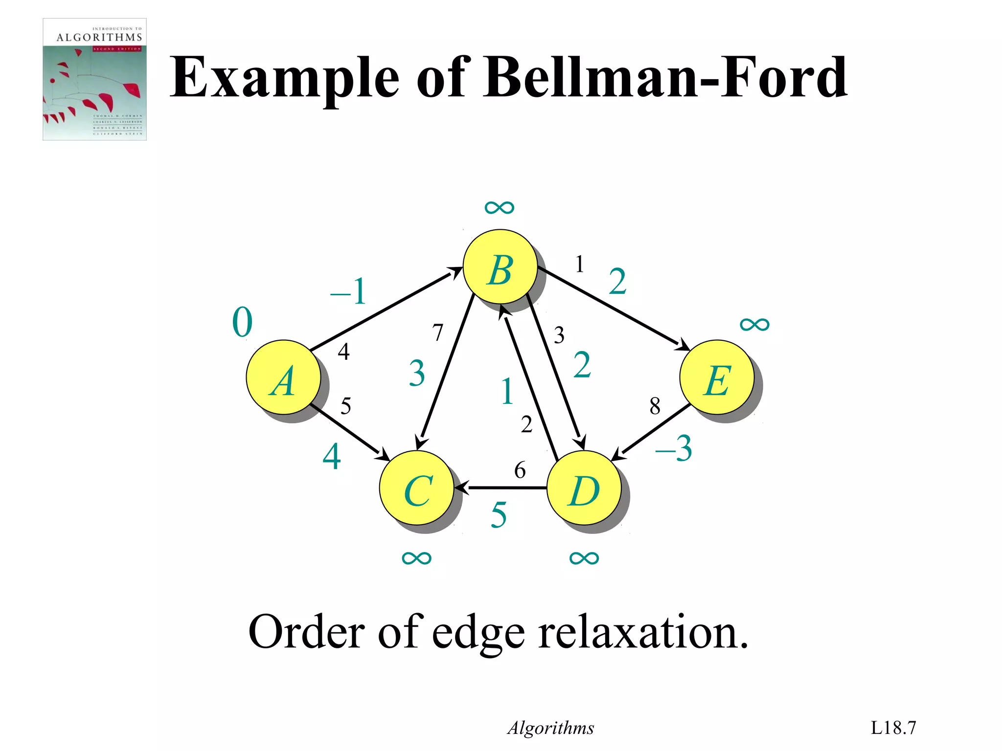
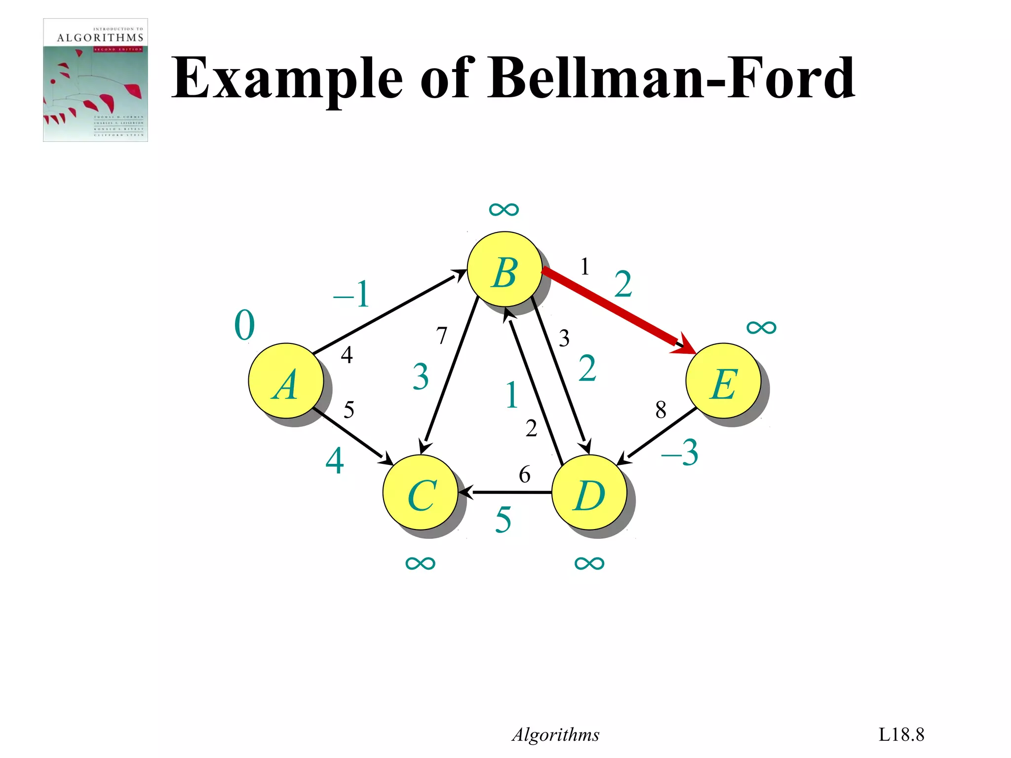
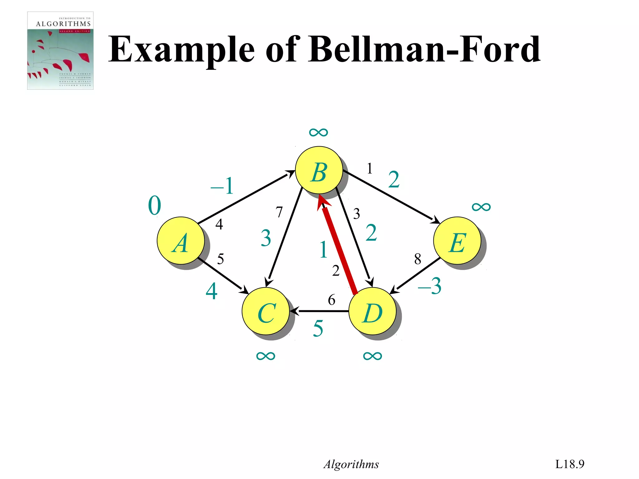
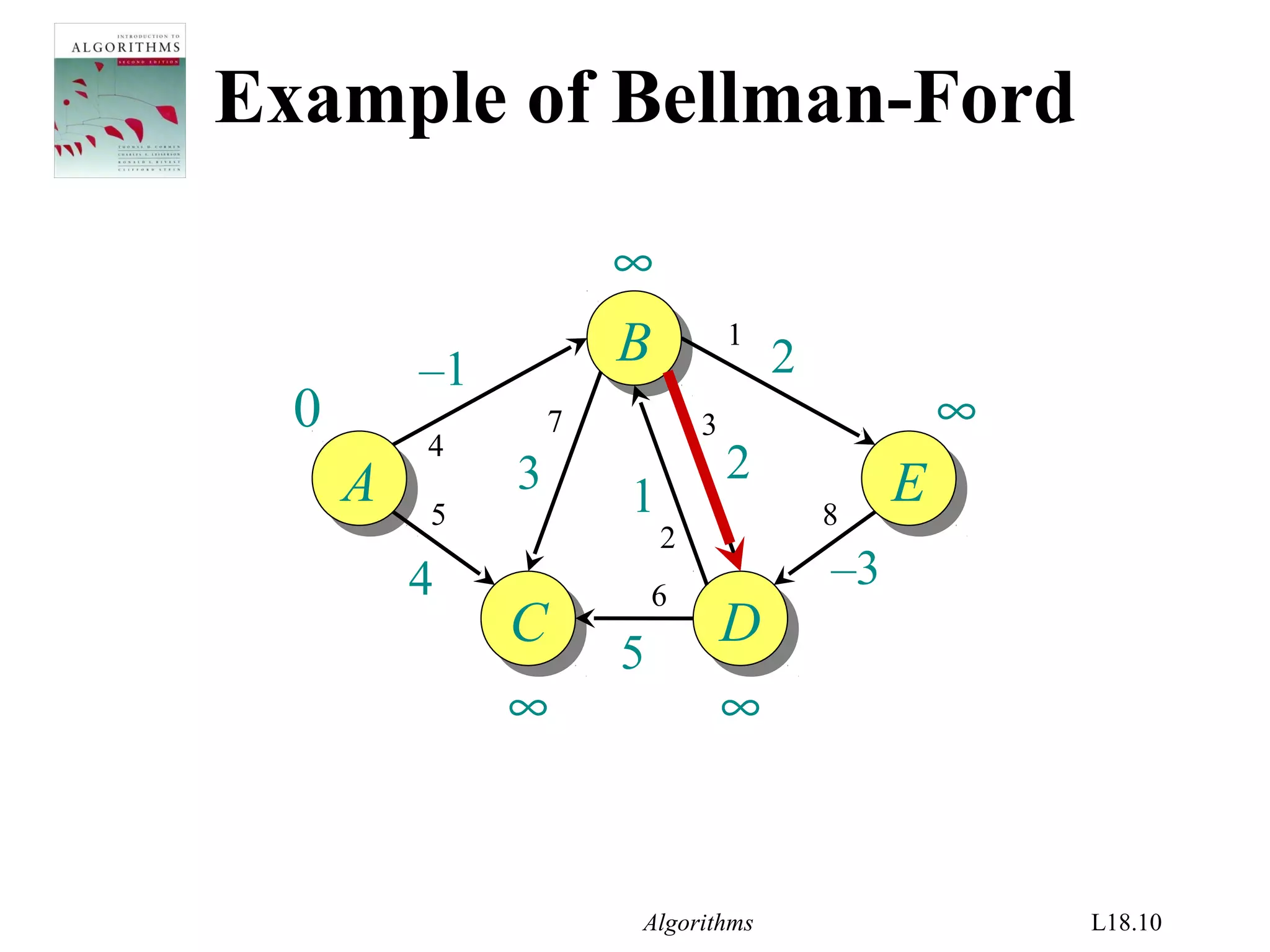
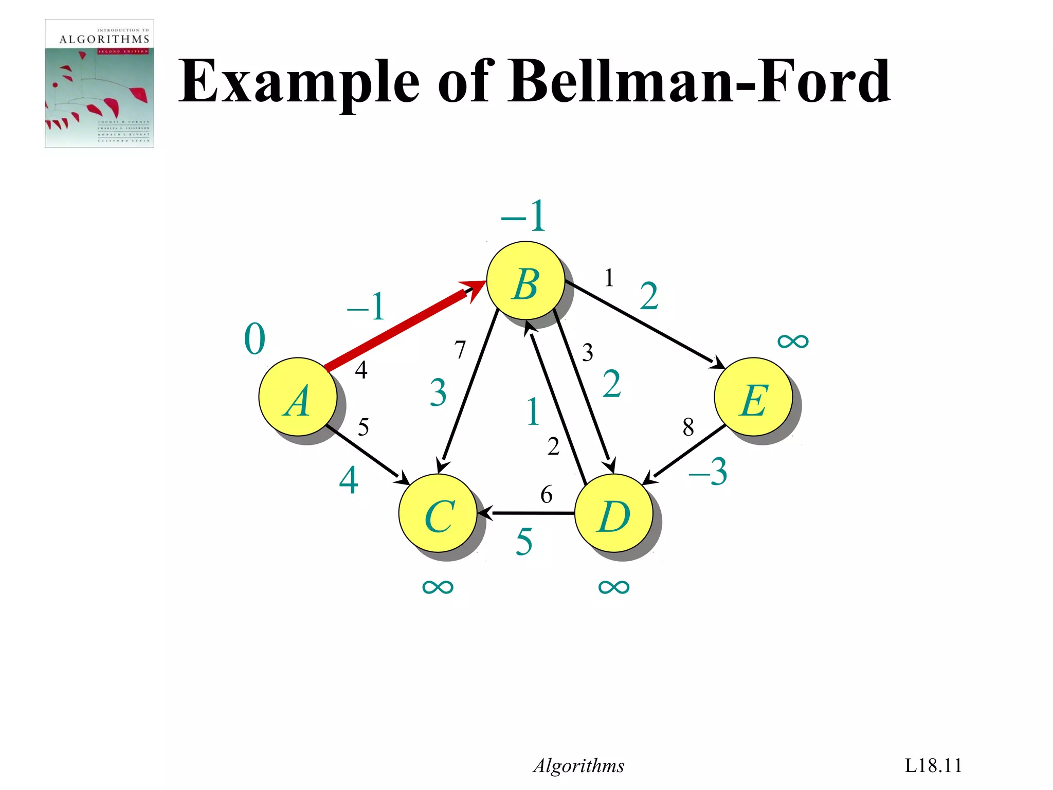
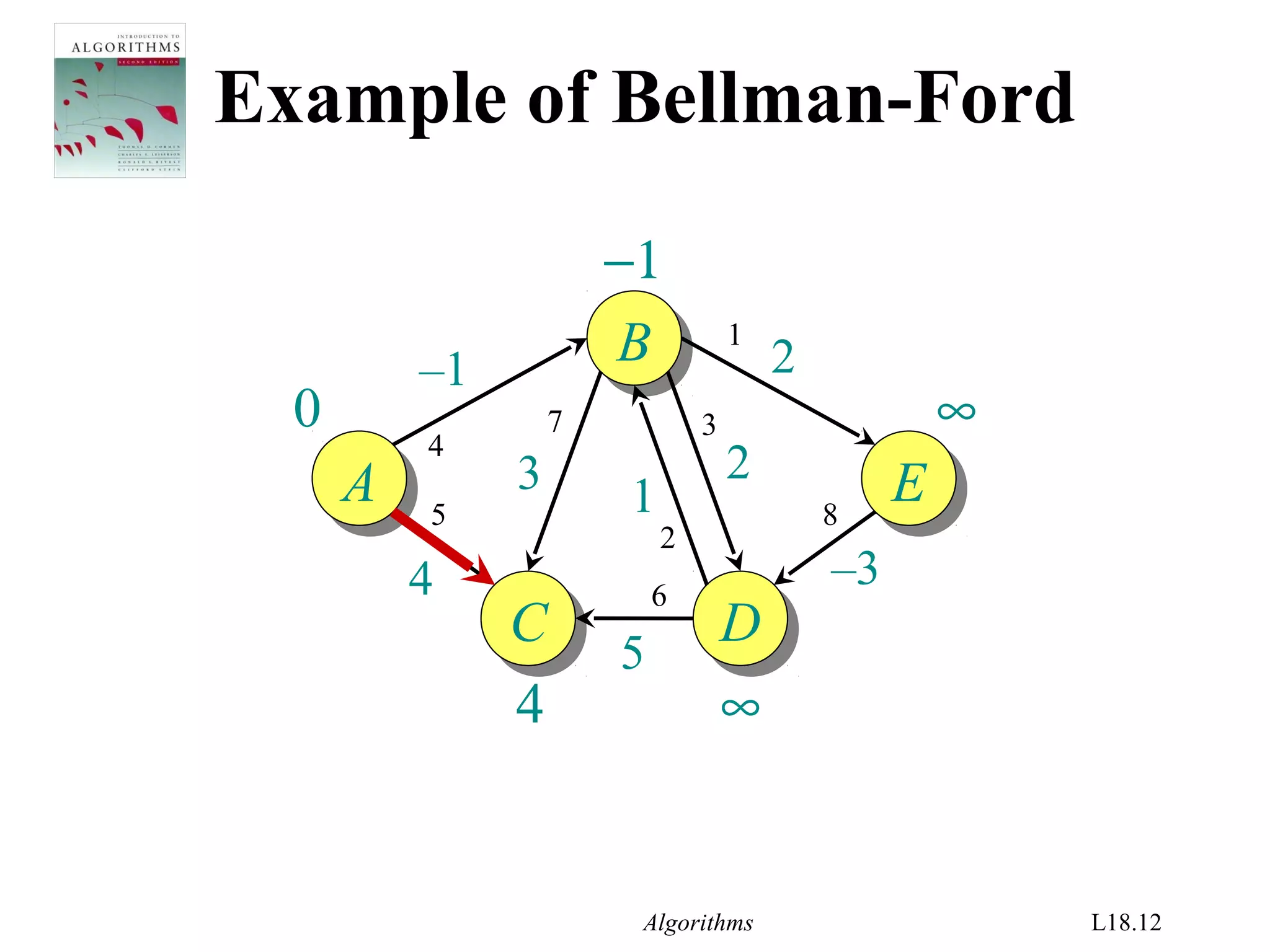
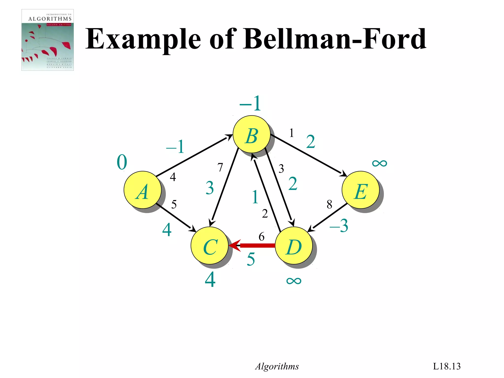
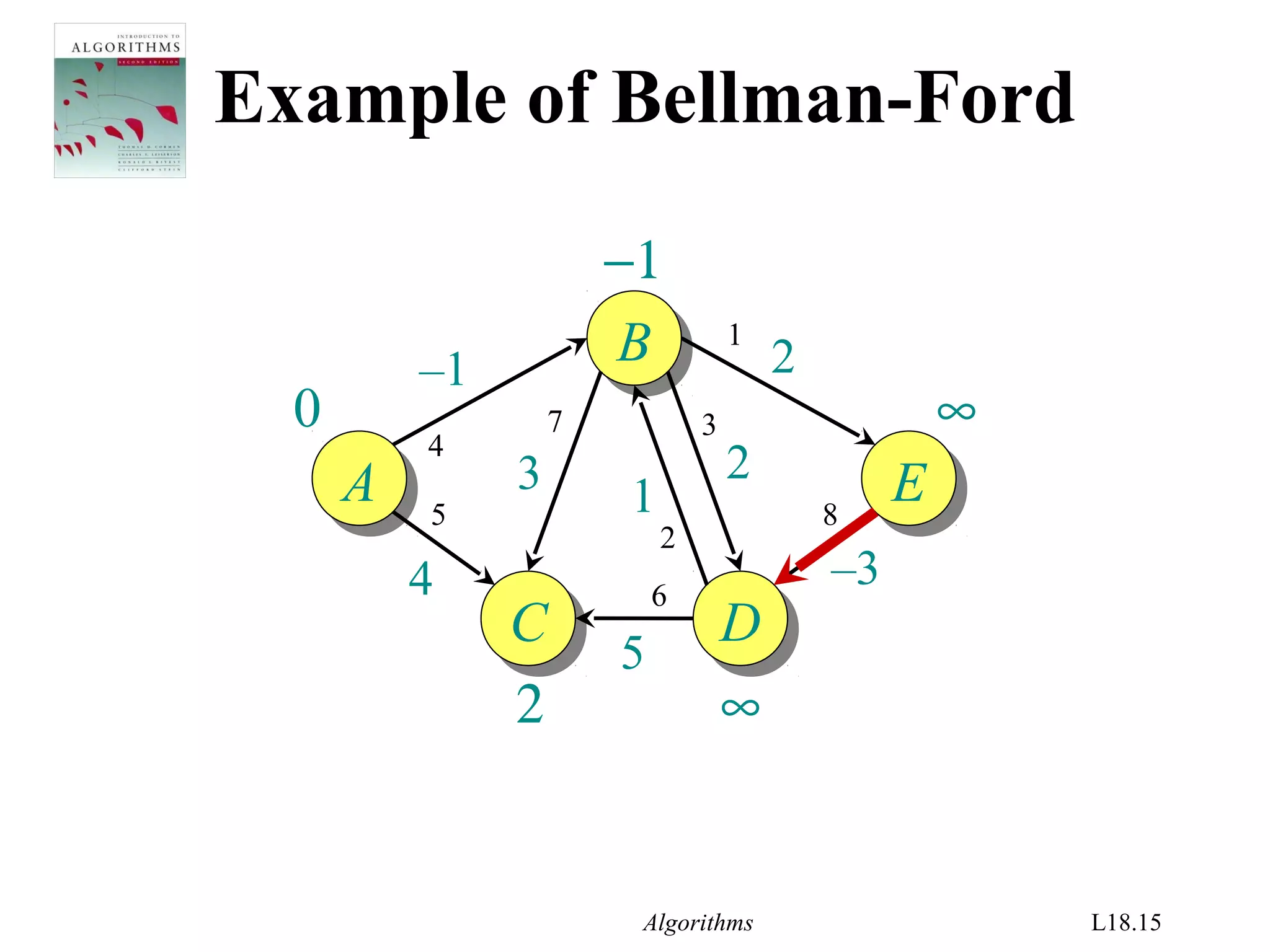
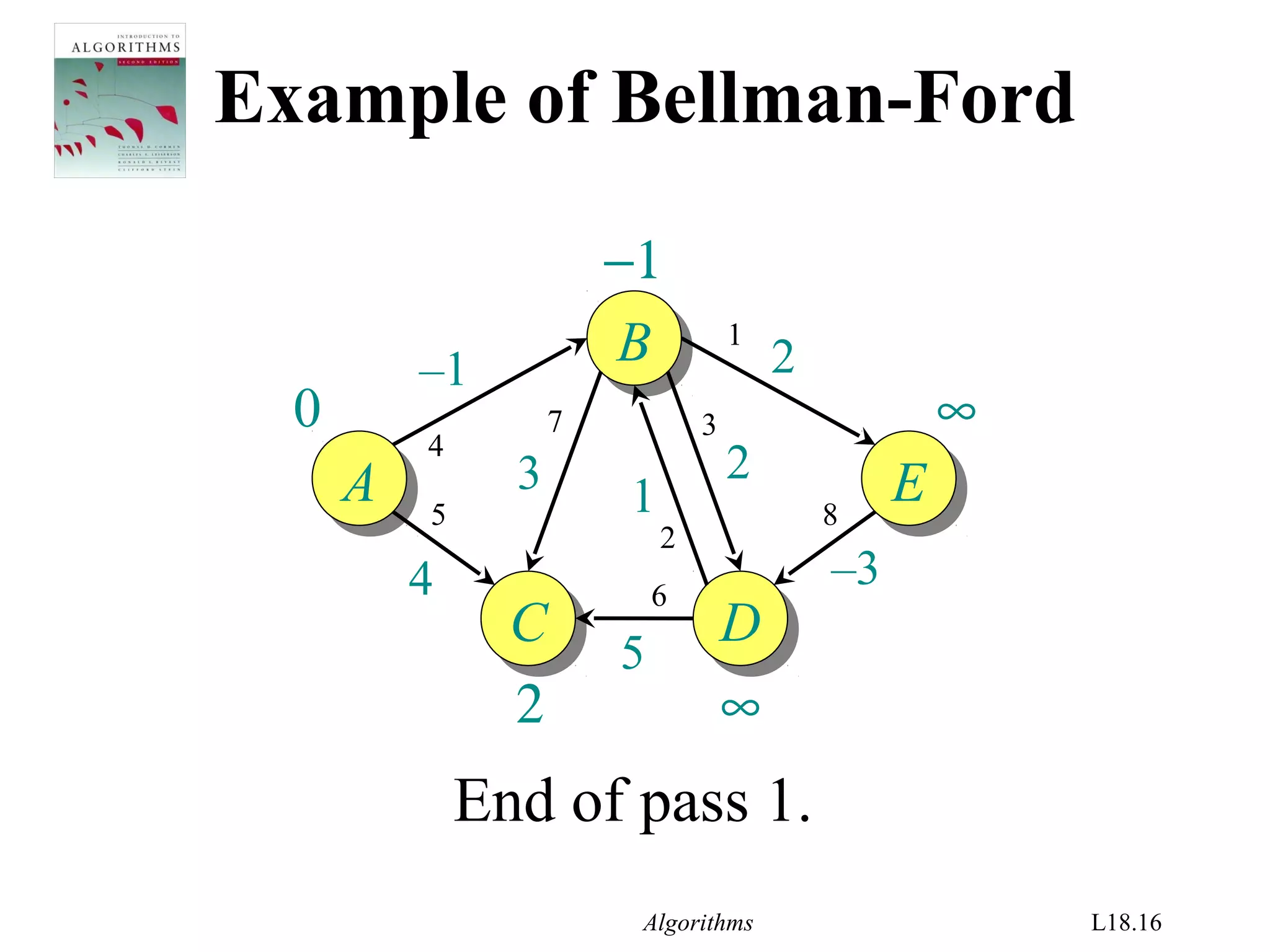
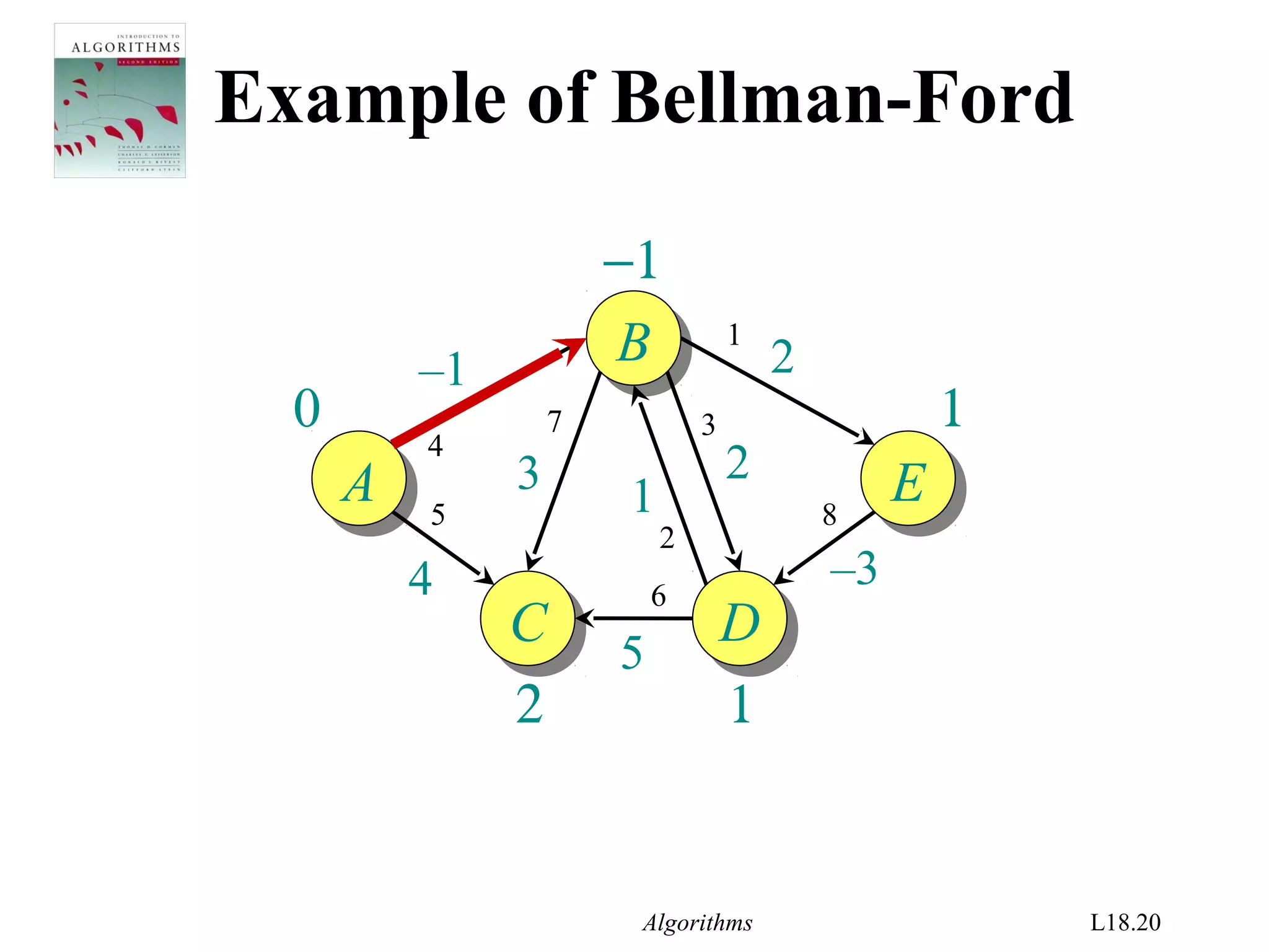
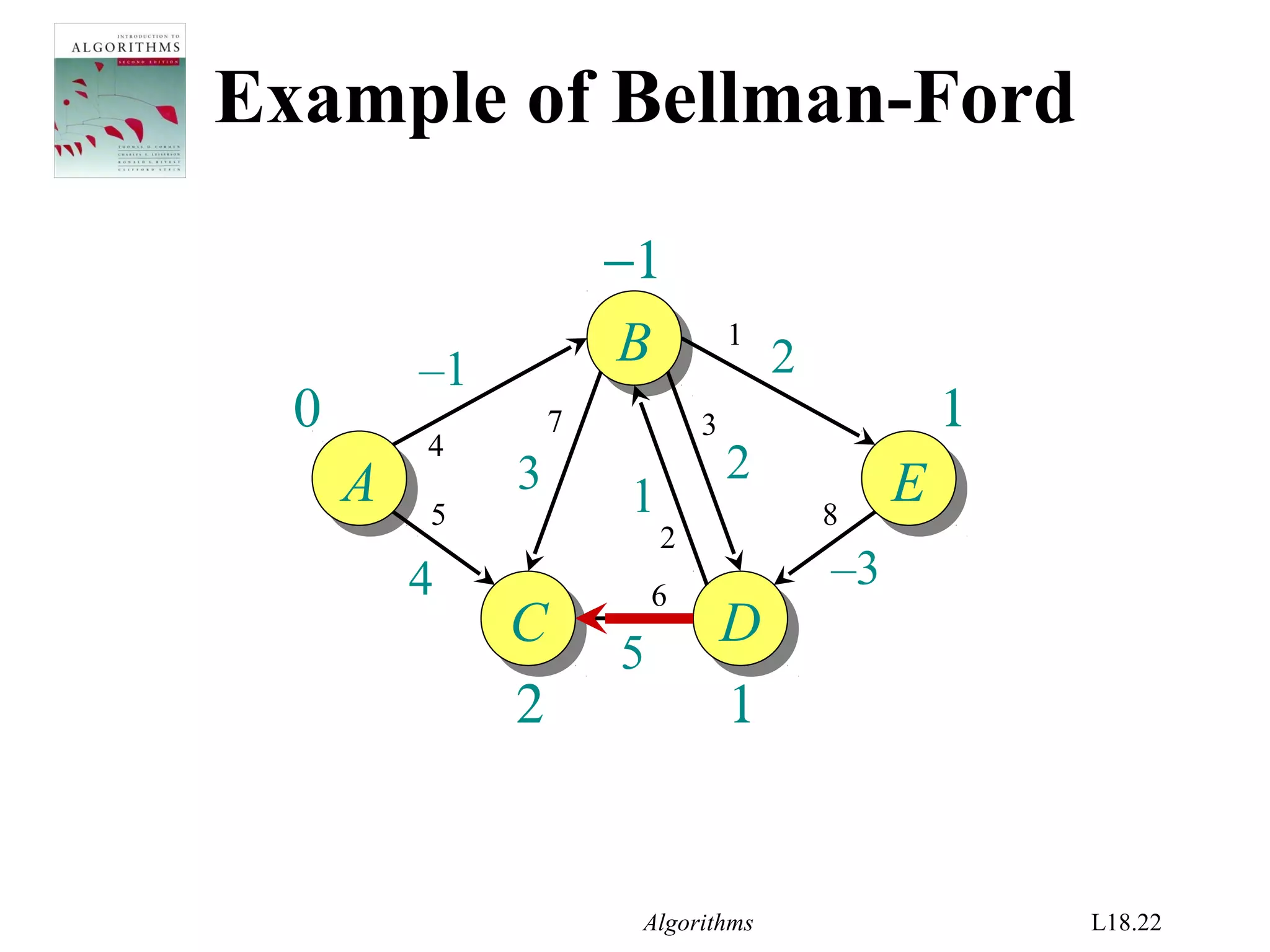
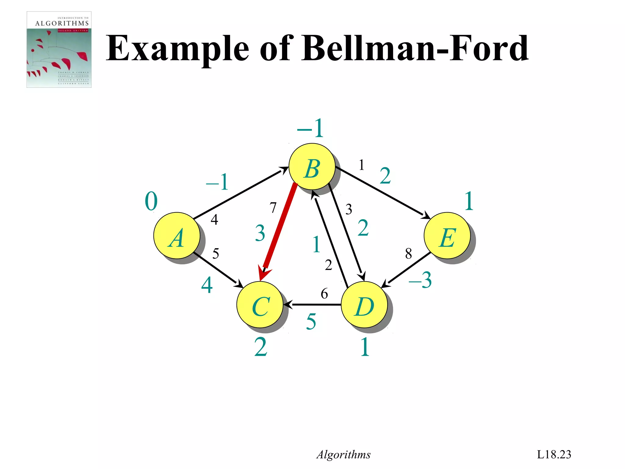
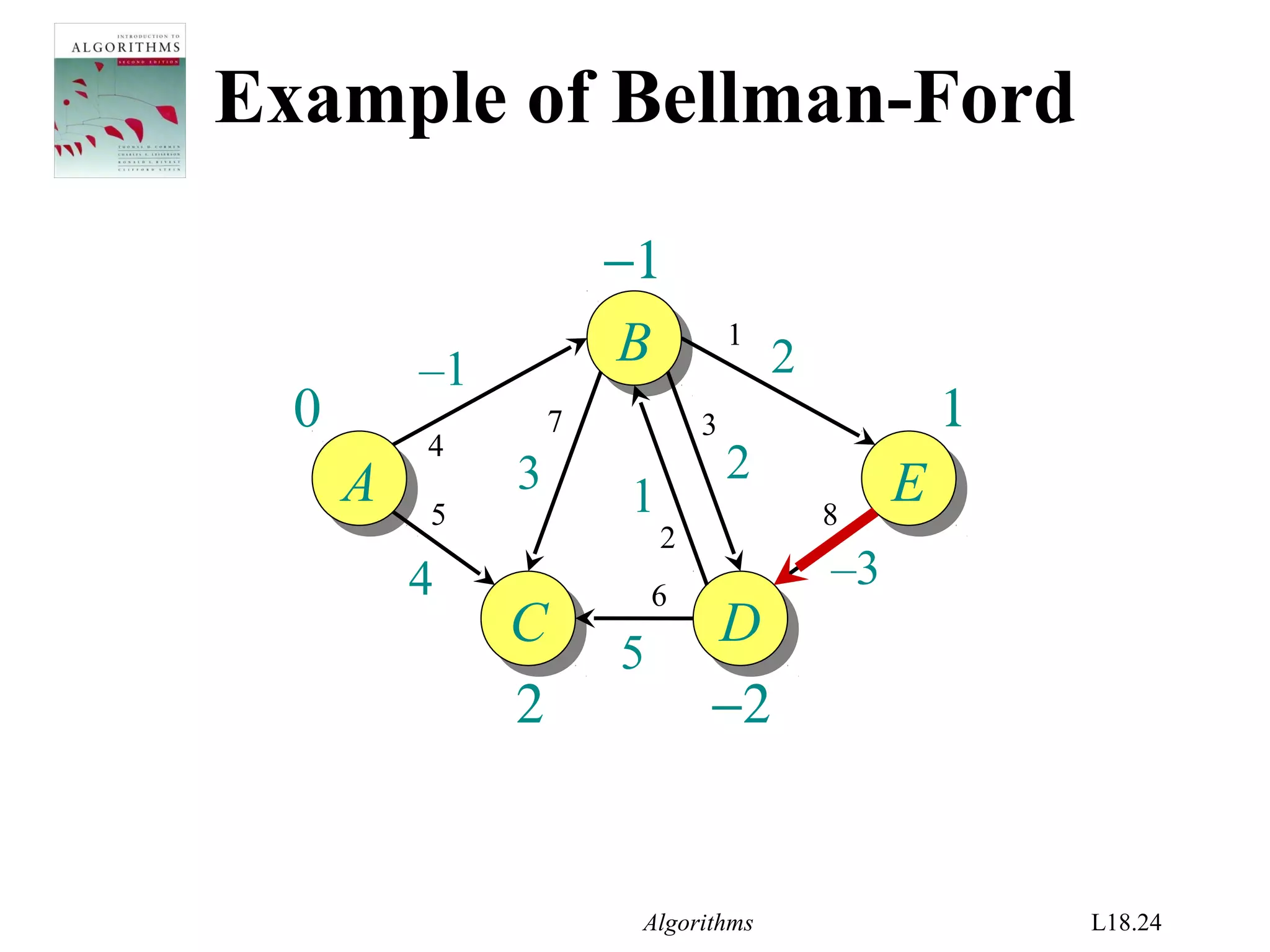
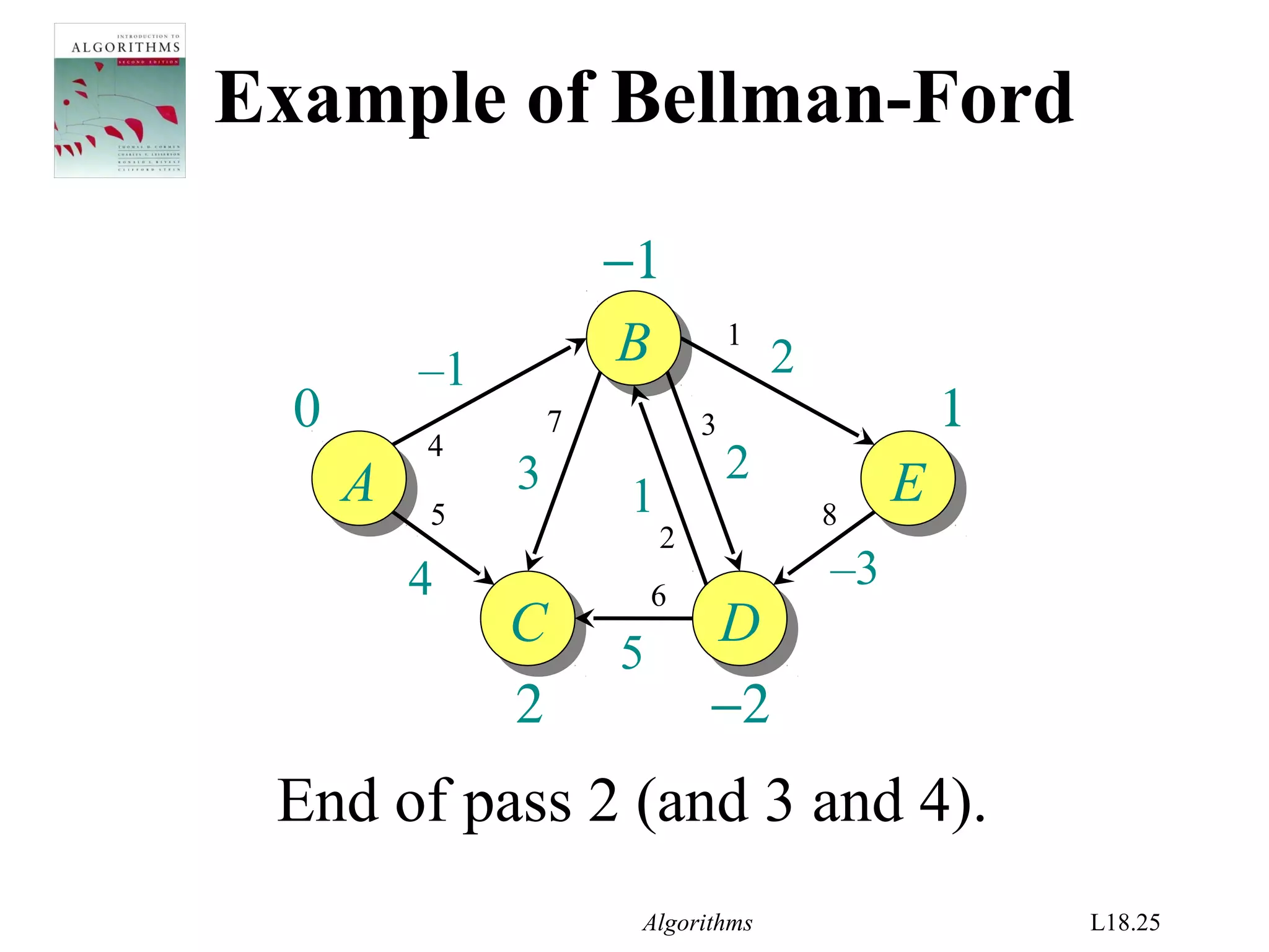
Bellman-Ford algorithm
d[s] ← 0
for each v ∈ V – {s}
do d[v] ← ∞
for i ← 1 to |V| – 1
do for each edge (u, v) ∈ E
do if d[v] > d[u] + w(u, v)
then d[v] ← d[u] + w(u, v)
for each edge (u, v) ∈ E
do if d[v] > d[u] + w(u, v)
then report that a negative-weight cycle exists
initialization
At the end, d[v] = δ(s, v), if no negative-weight cycles.
Time = O(VE).
relaxation
step](https://image.slidesharecdn.com/shortest-paths-bf-140416091424-phpapp02/75/Bellman-Ford-s-Algorithm-4-2048.jpg)


![Algorithms L18.26
Correctness
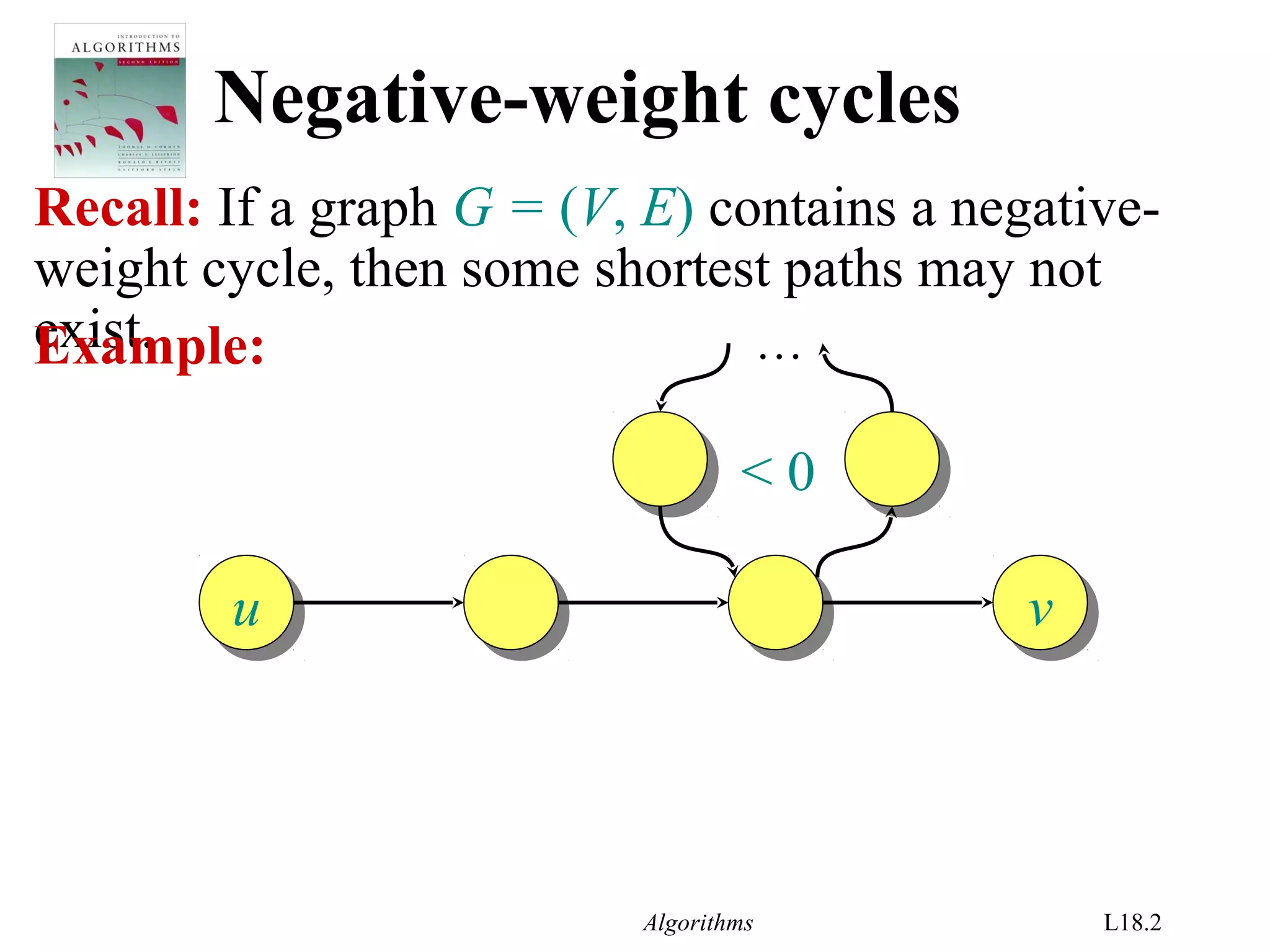
Theorem. If G = (V, E) contains no negative-
weight cycles, then after the Bellman-Ford
algorithm executes, d[v] = δ(s, v) for all v ∈ V.](https://image.slidesharecdn.com/shortest-paths-bf-140416091424-phpapp02/75/Bellman-Ford-s-Algorithm-26-2048.jpg)
![Algorithms L18.27
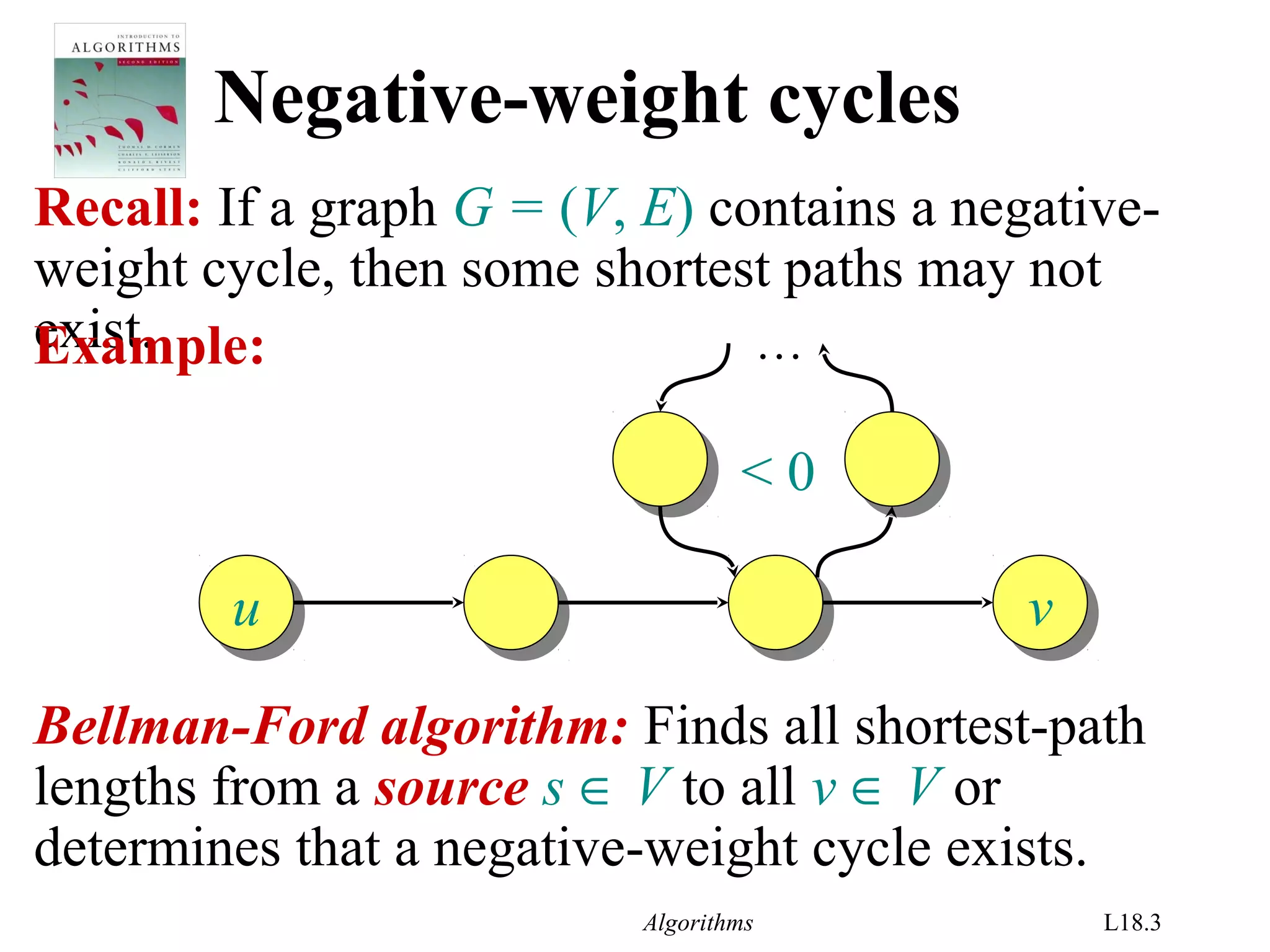
Correctness
Theorem. If G = (V, E) contains no negative-
weight cycles, then after the Bellman-Ford
algorithm executes, d[v] = δ(s, v) for all v ∈ V.
Proof. Let v ∈ V be any vertex, and consider a shortest
path p from s to v with the minimum number of edges.
v1
v1
v2
v2
v3
v3 vk
vk
v0
v0
…
s
v
p:
Since p is a shortest path, we have
δ(s, vi) = δ(s, vi–1) + w(vi–1, vi) .](https://image.slidesharecdn.com/shortest-paths-bf-140416091424-phpapp02/75/Bellman-Ford-s-Algorithm-27-2048.jpg)
![Algorithms L18.28
Correctness (continued)
v1
v1
v2
v2
v3
v3 vk
vk
v0
v0
…
s
v
p:
Initially, d[v0] = 0 = δ(s, v0), and d[v0] is unchanged by
subsequent relaxations (because of the lemma from
Lecture 14 that d[v] ≥ δ(s, v)).
• After 1 pass through E, we have d[v1] = δ(s, v1).
• After 2 passes through E, we have d[v2] = δ(s, v2).
• After k passes through E, we have d[vk] = δ(s, vk).
Since G contains no negative-weight cycles, p is simple.
Longest simple path has ≤ |V| – 1 edges.](https://image.slidesharecdn.com/shortest-paths-bf-140416091424-phpapp02/75/Bellman-Ford-s-Algorithm-28-2048.jpg)
![Algorithms L18.29
Detection of negative-weight
cycles
Corollary. If a value d[v] fails to converge after
|V| – 1 passes, there exists a negative-weight
cycle in G reachable from s.](https://image.slidesharecdn.com/shortest-paths-bf-140416091424-phpapp02/75/Bellman-Ford-s-Algorithm-29-2048.jpg)

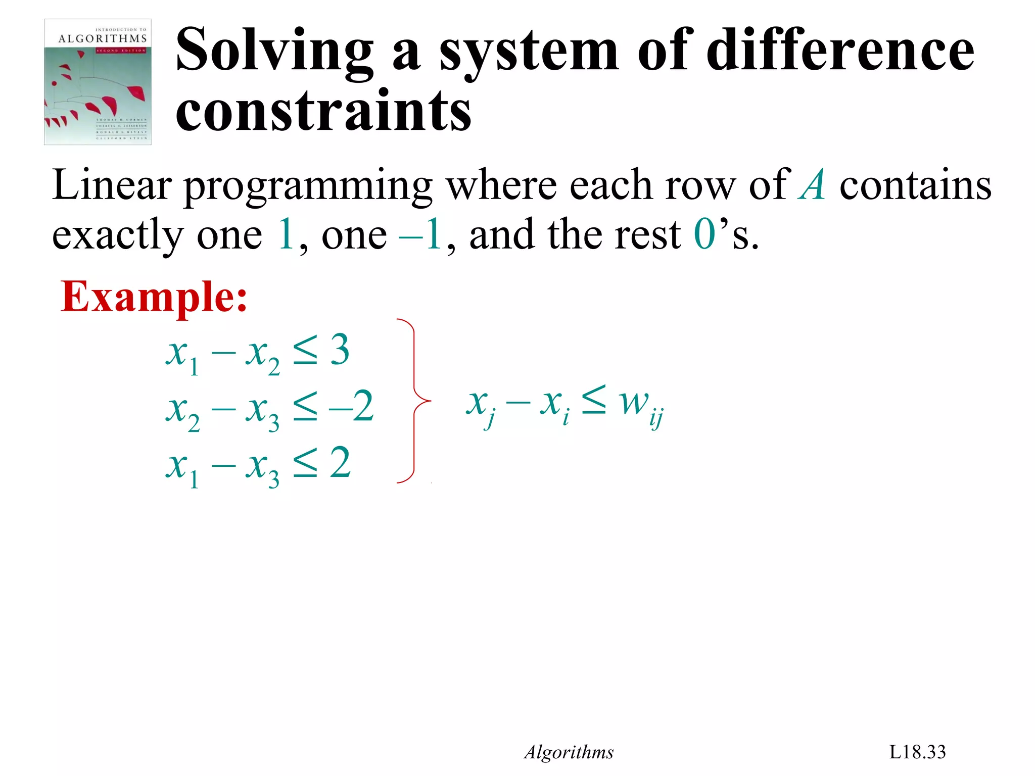
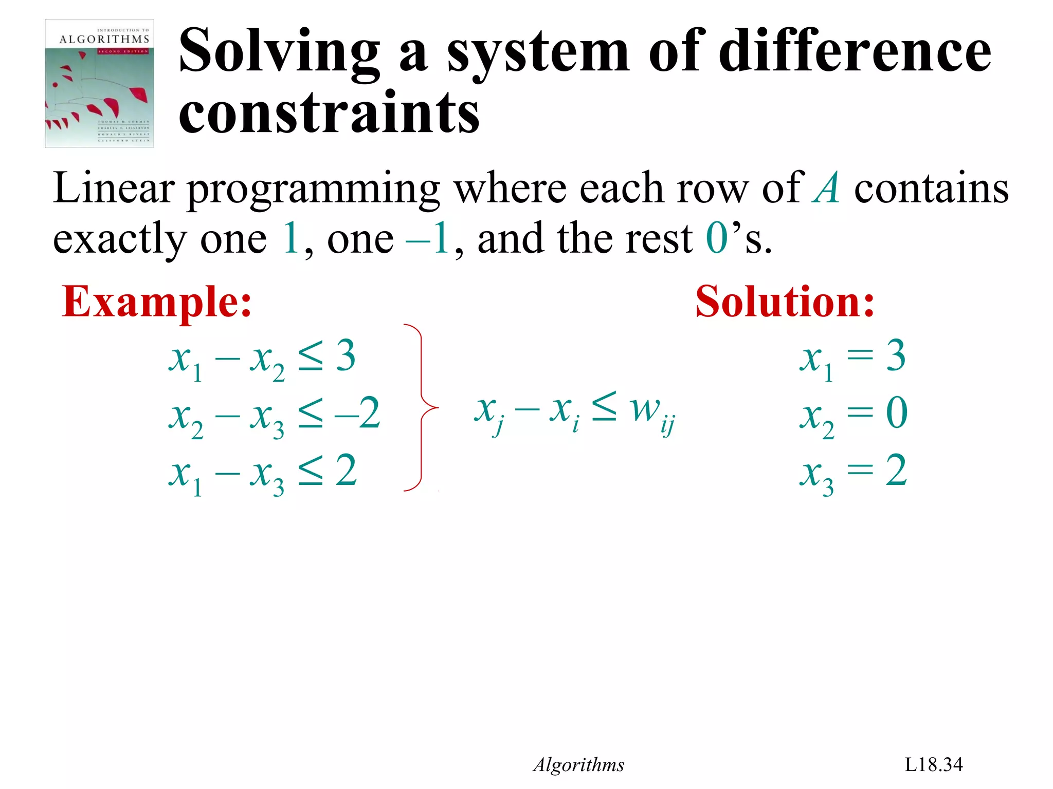
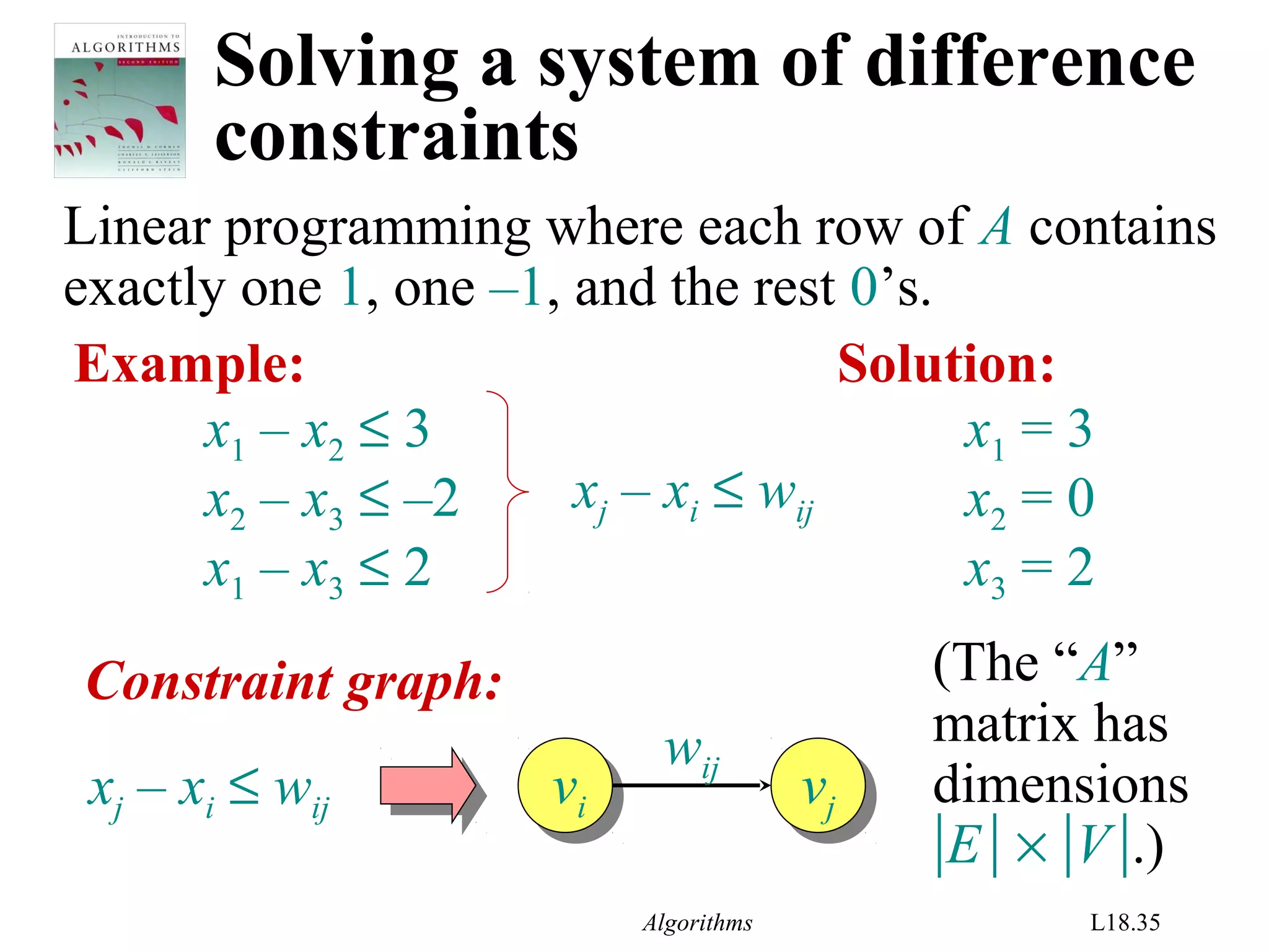
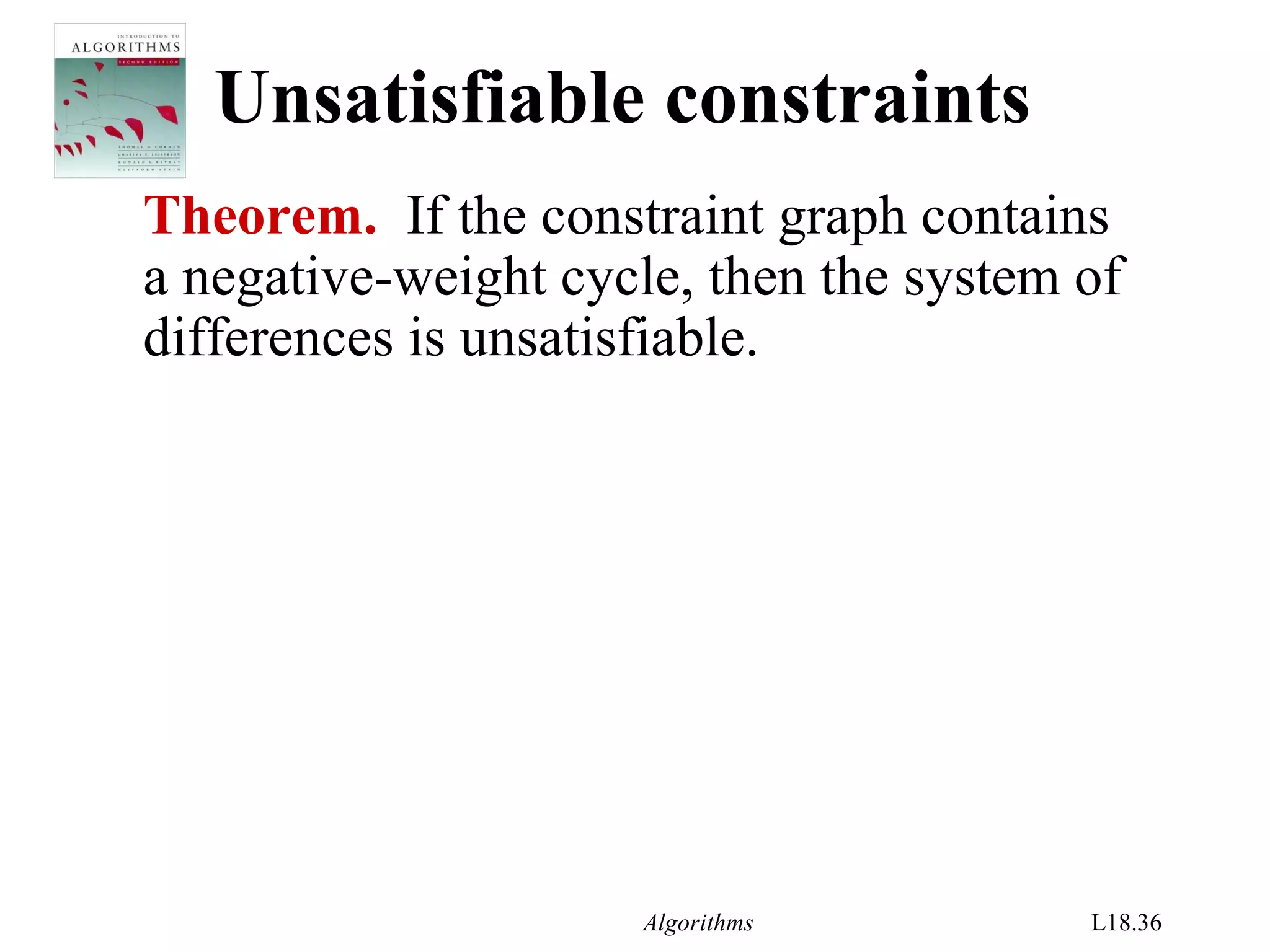
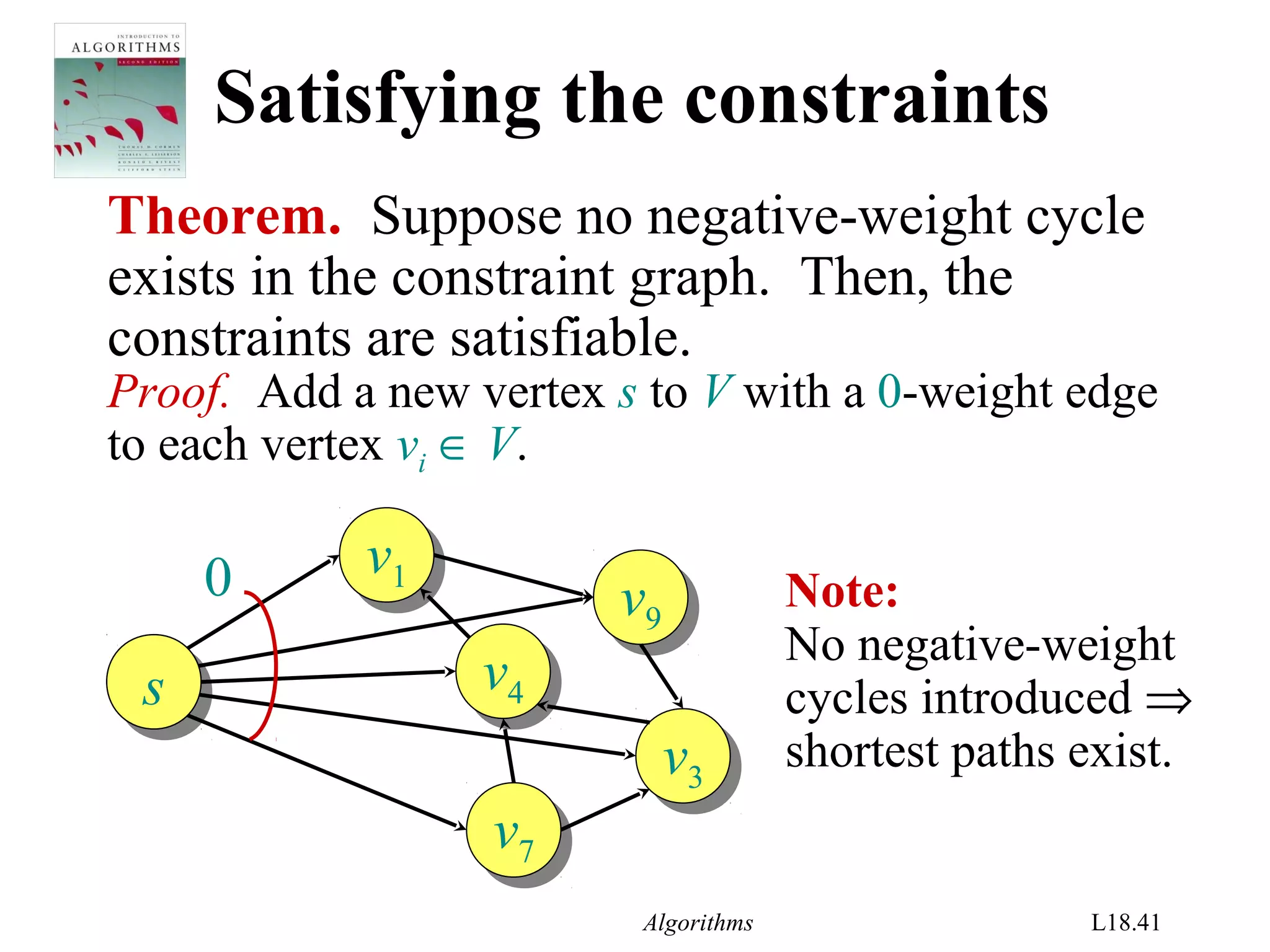
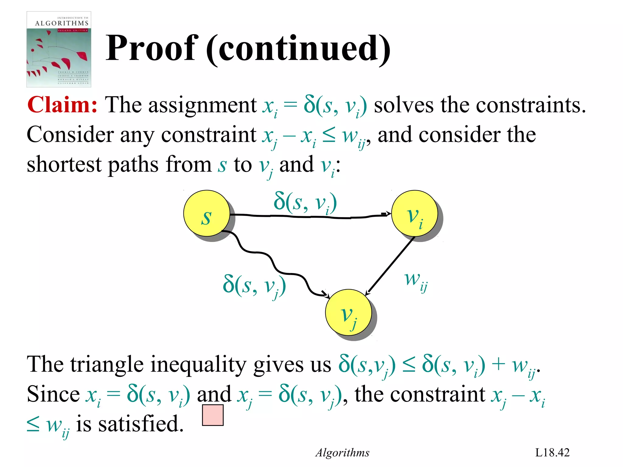


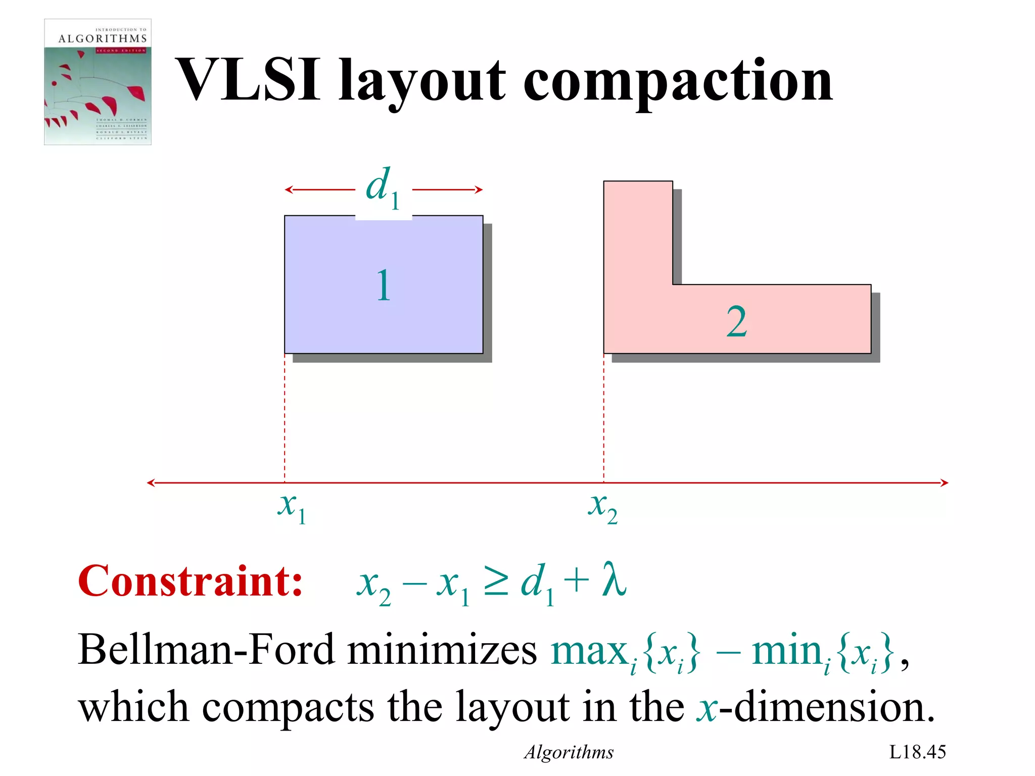

The document covers the Bellman-Ford algorithm for finding shortest paths in graphs, including its ability to detect negative-weight cycles. It includes specific algorithmic steps, examples, and discusses its applications in linear programming and VLSI layout compaction. Additionally, it emphasizes the algorithm's efficiency and correctness under certain conditions, along with methodologies for solving systems of difference constraints.