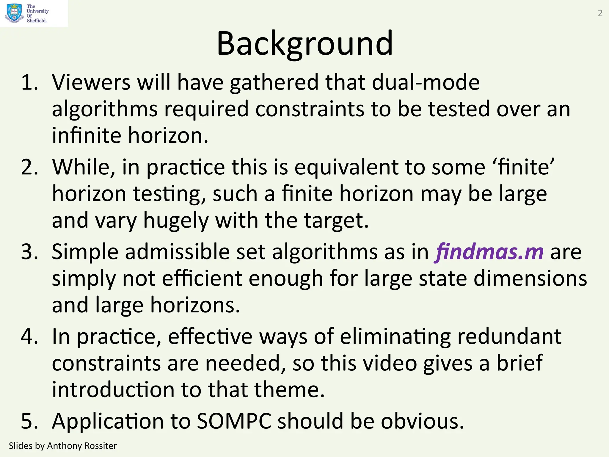
Slides by Anthony Rossiter
1
CHAPTER 5
Predictive Control with constraints 14
Alternative admissible set algorithms
Anthony Rossiter
Slides by Anthony Rossiter
2
Background
1. Viewers will have gathered that dual-mode
algorithms required constraints to be tested over an
infinite horizon.
2. While, in practice this is equivalent to some ‘finite’
horizon testing, such a finite horizon may be large
and vary hugely with the target.
3. Simple admissible set algorithms as in findmas.m are
simply not efficient enough for large state dimensions
and large horizons.
4. In practice, effective ways of eliminating redundant
constraints are needed, so this video gives a brief
introduction to that theme.
5. Application to SOMPC should be obvious.
Slides by Anthony Rossiter
3
Maximal admissible set
• Express predictions in the form:
• Express constraints at each sample in the form:
A critical requirement to ensure convergence is that
the asymptotic point was strictly inside the MCAS,
not on the boundary.
k
k Ax
x 
1
f
Gxk 
0
lim 


k
k A
f

0
0
,
;
lim 




 

t
Fx
x
x ss
ss
k
k
t
Fxk 
Slides by Anthony Rossiter
4
Maximal admissible set
• Let the inequalities be given for
a specified horizon ‘n’:
• Try and find a value ‘x’ which
violates constraints at ‘n+1’ but
satisfies constraints earlier on. 
t
k
F
n
f
f
f
f
x
GA
GA
GA
G






































2
1. If we cannot force a violation, then ‘n’ is large enough.
2. If we can, increase n and try again.
 ,
.
.
max 1
t
Fx
t
s
x
GA k
n
x


Slides by Anthony Rossiter
5
Weakness of findmas.m
The number of inequalities grows very quickly.

t
k
F
n
f
f
f
f
x
GA
GA
GA
G






































2

t
k
F
n
n
f
f
f
f
x
GA
GA
GA
GA
G








































 


1
2

t
k
F
n
n
n f
f
f
f
x
GA
GA
GA
GA
GA
G










































 

 


2
1
2
In practice, although we need to increase the horizon,
many of the earlier rows may be redundant and can be
removed, ‘on-the-go’.
Perhaps only one row of GAn+i
is active and needs adding!
Slides by Anthony Rossiter
6
Alternative approach
In this approach one considers the problem
backwards beginning form sample constraints.
What constraint on x(k) ensures x(k+1) also meets
sample constraints.
 
t
n
k
F
T
n
T
T
f
f
f
x
g
g
g





























2
1
2
1
Seed with
F=G and t=f. k
k Ax
x 
1













t
t
x
FA
F
k
Treat this as the new G and
f and repeat!
Slides by Anthony Rossiter
7
Alternative approach cont.
A smart viewer will note that in essence we have
done the following:
 
t
n
k
F
T
n
T
T
f
f
f
x
g
g
g





























2
1
2
1
From this an alternative and simple iteration
can be seen (see Pluymers et al).

t
n
k
F
T
T
T
n
T
T
f
f
f
f
f
x
A
g
A
g
g
g
g






















































2
1
2
1
2
1
2
1










t
n
n
n
k
F
T
n
T
n
T
n
T
T
f
f
f
f
f
x
g
g
g
g
g



















































2
1
2
1
2
1
2
1
Slides by Anthony Rossiter
8
Alternative approach cont.
Basic iteration:
 
t
n
k
F
T
n
T
T
f
f
f
x
g
g
g





























2
1
2
1
STEP 1

t
n
k
F
T
T
n
T
T
f
f
f
f
x
A
g
g
g
g

































1
2
1
1
2
1













t
n
n
n
k
F
T
T
n
T
n
T
T
f
f
f
f
f
x
A
g
g
g
g
g










































2
1
2
1
2
1
2
1
STEP 2

t
r
m
k
F
T
r
T
m
T
T
f
f
f
f
x
A
g
g
g
g






































2
1
2
1
STEP r
Keep going until
all rows of F have
been used. (r=m)
New row retained
only if active.
Clean out
redundant
rows from
time to time.
Slides by Anthony Rossiter
9
MATLAB code
The relevant file is in the constraints examples
folder. [Modified from an original by Bert Pluymers]
Called construct_mas.m
e.g. construct_mas(A,G,f)
LACK of convergence is usually linked to the user
entering a state transition matrix ‘A’ which does not
have stable eigenvalues.
Also, the code does not check for ‘feasibility’
Slides by Anthony Rossiter
10
video5_14_example1.m
Simple box sample constraints and state transition
matrix.
MCAS has 8 inequalities.
-10 -8 -6 -4 -2 0 2 4 6 8 10
-10
-8
-6
-4
-2
0
2
4
6
8
10
MCAS
Slides by Anthony Rossiter
11
video5_14_example2.m
Simple box sample constraints and state transition
matrix.
MCAS has
10 inequalities.
-10 -5 0 5 10
-10
-5
0
5
10
MCAS and state evolutions
Sample constraints
MCAS
Slides by Anthony Rossiter
12
video5_14_example3.m
3 states, sample constraints an asymetric box.
-2
-1
0
1
-3
-2
-1
0
1
-4
-3
-2
-1
0
1
Sample constraints
-1
-0.5
0
0.5
1
-2
-1
0
1
-4
-3
-2
-1
0
1
MCAS
Slides by Anthony Rossiter
13
Remark
The SOMPC tracking problem separated constraints
into two parts.
We can easily modify our admissible set algorithm to
deal with this by starting the iteration on rows in G2
and thus excluding G1.
construct_mas_tracking(A,G1,G2,f1,f2)













2
1
2
1
f
f
Z
G
G
k
k
f
Z
G k 
 ,
2
2
only
k
f
Z
G k
0
,
1
1


k
k AZ
Z 
1
Slides by Anthony Rossiter
14
video5_14_example4.m
Same as example 1 but with extra state that does
not change and has simple box limits.
MCAS now has 10 inequalities.
-10
-5
0
5
10
-10
-5
0
5
10
-1
-0.5
0
0.5
1
MCAS
-10 -8 -6 -4 -2 0 2 4 6 8 10
-10
-8
-6
-4
-2
0
2
4
6
8
10
MCAS
Slides by Anthony Rossiter
15
video5_14_example5.m
Same as example2 but an extra state which does
not change.
MCAS now has 12 inequalities (2 more).
-10 -5 0 5 10
-10
-5
0
5
10
MCAS and state evolutions
Sample constraints
MCAS
-5
0
5
-10
-5
0
5
10
-1
-0.5
0
0.5
1
MCAS
Slides by Anthony Rossiter
16
video5_14_example6.m
Same as example3
Now has 4 states so we cannot plot.
Again, MCAS has 2 extra constraints associated to
the inequalities which are fixed at the outset.
Slides by Anthony Rossiter
17
WARNING
• The autonomous model for OMPC includes states
c(k+i) which only impact several samples into the
future.
• This means, they have no impact on first few
iterations of the algorithm and thus can take any
values.
• This leads to ‘unbounded’ results from the linear
programme.
Code must have suitable error catching for this case
which is always going to occur in SOMPC.
Slides by Anthony Rossiter
18
Summary
1. This video has shown how more efficient
admissible set algorithms can be coded.
2. A key part of these algorithm is the addition of
just one new row at a time.
3. Secondly, there are regular checks for and
removal of redundant constraints.
4. Next we apply this to the SOMPC algorithm and
explore the typical number of inequalities
required for different scenarios.
© 2014 University of Sheffield
This work is licensed under the Creative Commons Attribution 2.0 UK: England & Wales Licence. To view a copy of this licence, visit
http://creativecommons.org/licenses/by/2.0/uk/ or send a letter to: Creative Commons, 171 Second Street, Suite 300, San Francisco, California 94105, USA.
It should be noted that some of the materials contained within this resource are subject to third party rights and any copyright notices must remain with these materials
in the event of reuse or repurposing.
If there are third party images within the resource please do not remove or alter any of the copyright notices or website details shown below the image.
(Please list details of the third party rights contained within this work.
If you include your institutions logo on the cover please include reference to the fact that it is a trade mark and all copyright in that image is reserved.)
Anthony Rossiter
Department of Automatic Control and
Systems Engineering
University of Sheffield
www.shef.ac.uk/acse

predictive control with constraints 5-14 - alternative admissible set algorithms.pptx

  • 1.
    Slides by AnthonyRossiter 1 CHAPTER 5 Predictive Control with constraints 14 Alternative admissible set algorithms Anthony Rossiter
  • 2.
    Slides by AnthonyRossiter 2 Background 1. Viewers will have gathered that dual-mode algorithms required constraints to be tested over an infinite horizon. 2. While, in practice this is equivalent to some ‘finite’ horizon testing, such a finite horizon may be large and vary hugely with the target. 3. Simple admissible set algorithms as in findmas.m are simply not efficient enough for large state dimensions and large horizons. 4. In practice, effective ways of eliminating redundant constraints are needed, so this video gives a brief introduction to that theme. 5. Application to SOMPC should be obvious.
  • 3.
    Slides by AnthonyRossiter 3 Maximal admissible set • Express predictions in the form: • Express constraints at each sample in the form: A critical requirement to ensure convergence is that the asymptotic point was strictly inside the MCAS, not on the boundary. k k Ax x  1 f Gxk  0 lim    k k A f  0 0 , ; lim         t Fx x x ss ss k k t Fxk 
  • 4.
    Slides by AnthonyRossiter 4 Maximal admissible set • Let the inequalities be given for a specified horizon ‘n’: • Try and find a value ‘x’ which violates constraints at ‘n+1’ but satisfies constraints earlier on.  t k F n f f f f x GA GA GA G                                       2 1. If we cannot force a violation, then ‘n’ is large enough. 2. If we can, increase n and try again.  , . . max 1 t Fx t s x GA k n x  
  • 5.
    Slides by AnthonyRossiter 5 Weakness of findmas.m The number of inequalities grows very quickly.  t k F n f f f f x GA GA GA G                                       2  t k F n n f f f f x GA GA GA GA G                                             1 2  t k F n n n f f f f x GA GA GA GA GA G                                                  2 1 2 In practice, although we need to increase the horizon, many of the earlier rows may be redundant and can be removed, ‘on-the-go’. Perhaps only one row of GAn+i is active and needs adding!
  • 6.
    Slides by AnthonyRossiter 6 Alternative approach In this approach one considers the problem backwards beginning form sample constraints. What constraint on x(k) ensures x(k+1) also meets sample constraints.   t n k F T n T T f f f x g g g                              2 1 2 1 Seed with F=G and t=f. k k Ax x  1              t t x FA F k Treat this as the new G and f and repeat!
  • 7.
    Slides by AnthonyRossiter 7 Alternative approach cont. A smart viewer will note that in essence we have done the following:   t n k F T n T T f f f x g g g                              2 1 2 1 From this an alternative and simple iteration can be seen (see Pluymers et al).  t n k F T T T n T T f f f f f x A g A g g g g                                                       2 1 2 1 2 1 2 1           t n n n k F T n T n T n T T f f f f f x g g g g g                                                    2 1 2 1 2 1 2 1
  • 8.
    Slides by AnthonyRossiter 8 Alternative approach cont. Basic iteration:   t n k F T n T T f f f x g g g                              2 1 2 1 STEP 1  t n k F T T n T T f f f f x A g g g g                                  1 2 1 1 2 1              t n n n k F T T n T n T T f f f f f x A g g g g g                                           2 1 2 1 2 1 2 1 STEP 2  t r m k F T r T m T T f f f f x A g g g g                                       2 1 2 1 STEP r Keep going until all rows of F have been used. (r=m) New row retained only if active. Clean out redundant rows from time to time.
  • 9.
    Slides by AnthonyRossiter 9 MATLAB code The relevant file is in the constraints examples folder. [Modified from an original by Bert Pluymers] Called construct_mas.m e.g. construct_mas(A,G,f) LACK of convergence is usually linked to the user entering a state transition matrix ‘A’ which does not have stable eigenvalues. Also, the code does not check for ‘feasibility’
  • 10.
    Slides by AnthonyRossiter 10 video5_14_example1.m Simple box sample constraints and state transition matrix. MCAS has 8 inequalities. -10 -8 -6 -4 -2 0 2 4 6 8 10 -10 -8 -6 -4 -2 0 2 4 6 8 10 MCAS
  • 11.
    Slides by AnthonyRossiter 11 video5_14_example2.m Simple box sample constraints and state transition matrix. MCAS has 10 inequalities. -10 -5 0 5 10 -10 -5 0 5 10 MCAS and state evolutions Sample constraints MCAS
  • 12.
    Slides by AnthonyRossiter 12 video5_14_example3.m 3 states, sample constraints an asymetric box. -2 -1 0 1 -3 -2 -1 0 1 -4 -3 -2 -1 0 1 Sample constraints -1 -0.5 0 0.5 1 -2 -1 0 1 -4 -3 -2 -1 0 1 MCAS
  • 13.
    Slides by AnthonyRossiter 13 Remark The SOMPC tracking problem separated constraints into two parts. We can easily modify our admissible set algorithm to deal with this by starting the iteration on rows in G2 and thus excluding G1. construct_mas_tracking(A,G1,G2,f1,f2)              2 1 2 1 f f Z G G k k f Z G k   , 2 2 only k f Z G k 0 , 1 1   k k AZ Z  1
  • 14.
    Slides by AnthonyRossiter 14 video5_14_example4.m Same as example 1 but with extra state that does not change and has simple box limits. MCAS now has 10 inequalities. -10 -5 0 5 10 -10 -5 0 5 10 -1 -0.5 0 0.5 1 MCAS -10 -8 -6 -4 -2 0 2 4 6 8 10 -10 -8 -6 -4 -2 0 2 4 6 8 10 MCAS
  • 15.
    Slides by AnthonyRossiter 15 video5_14_example5.m Same as example2 but an extra state which does not change. MCAS now has 12 inequalities (2 more). -10 -5 0 5 10 -10 -5 0 5 10 MCAS and state evolutions Sample constraints MCAS -5 0 5 -10 -5 0 5 10 -1 -0.5 0 0.5 1 MCAS
  • 16.
    Slides by AnthonyRossiter 16 video5_14_example6.m Same as example3 Now has 4 states so we cannot plot. Again, MCAS has 2 extra constraints associated to the inequalities which are fixed at the outset.
  • 17.
    Slides by AnthonyRossiter 17 WARNING • The autonomous model for OMPC includes states c(k+i) which only impact several samples into the future. • This means, they have no impact on first few iterations of the algorithm and thus can take any values. • This leads to ‘unbounded’ results from the linear programme. Code must have suitable error catching for this case which is always going to occur in SOMPC.
  • 18.
    Slides by AnthonyRossiter 18 Summary 1. This video has shown how more efficient admissible set algorithms can be coded. 2. A key part of these algorithm is the addition of just one new row at a time. 3. Secondly, there are regular checks for and removal of redundant constraints. 4. Next we apply this to the SOMPC algorithm and explore the typical number of inequalities required for different scenarios.
  • 19.
    © 2014 Universityof Sheffield This work is licensed under the Creative Commons Attribution 2.0 UK: England & Wales Licence. To view a copy of this licence, visit http://creativecommons.org/licenses/by/2.0/uk/ or send a letter to: Creative Commons, 171 Second Street, Suite 300, San Francisco, California 94105, USA. It should be noted that some of the materials contained within this resource are subject to third party rights and any copyright notices must remain with these materials in the event of reuse or repurposing. If there are third party images within the resource please do not remove or alter any of the copyright notices or website details shown below the image. (Please list details of the third party rights contained within this work. If you include your institutions logo on the cover please include reference to the fact that it is a trade mark and all copyright in that image is reserved.) Anthony Rossiter Department of Automatic Control and Systems Engineering University of Sheffield www.shef.ac.uk/acse