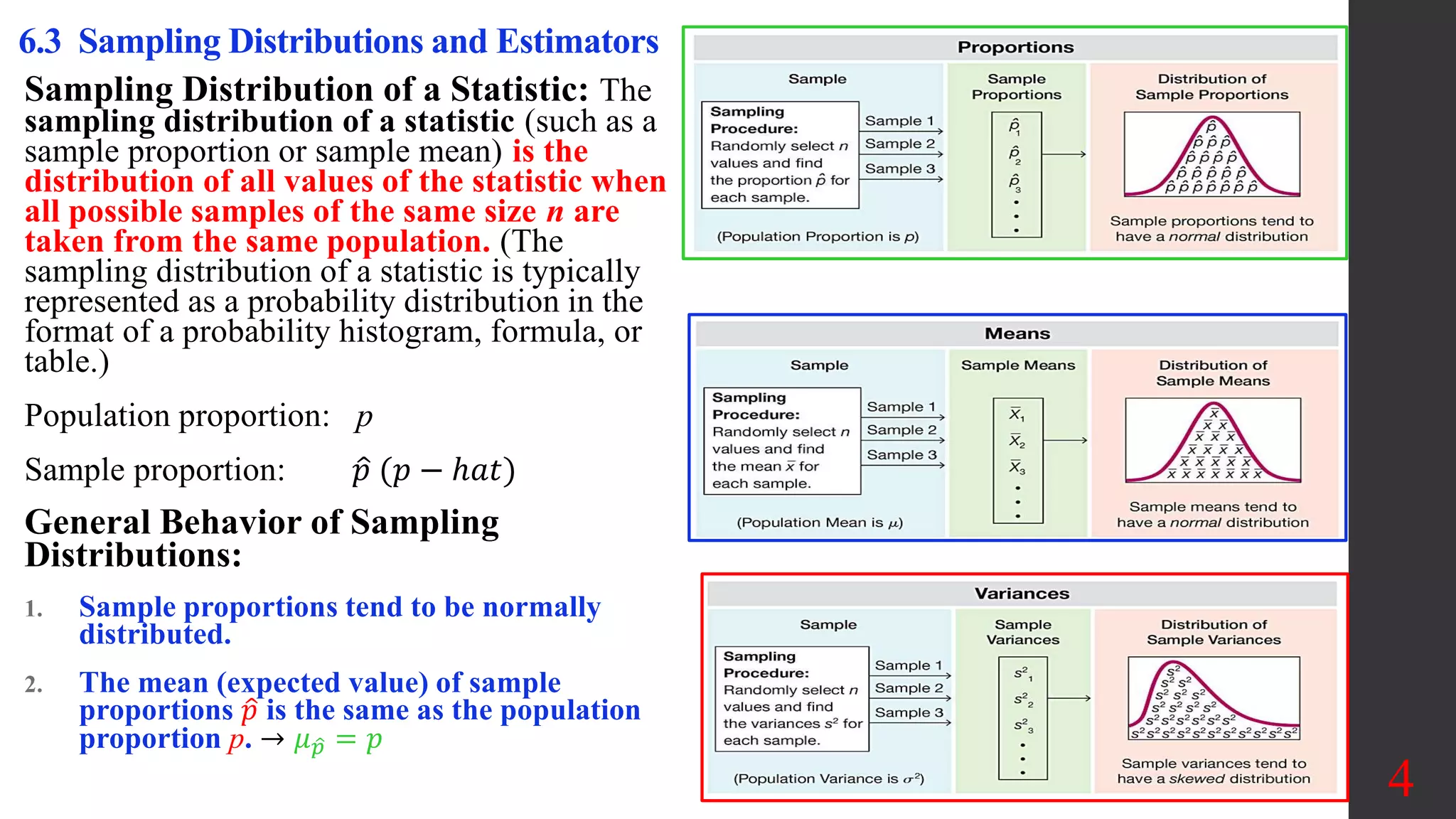
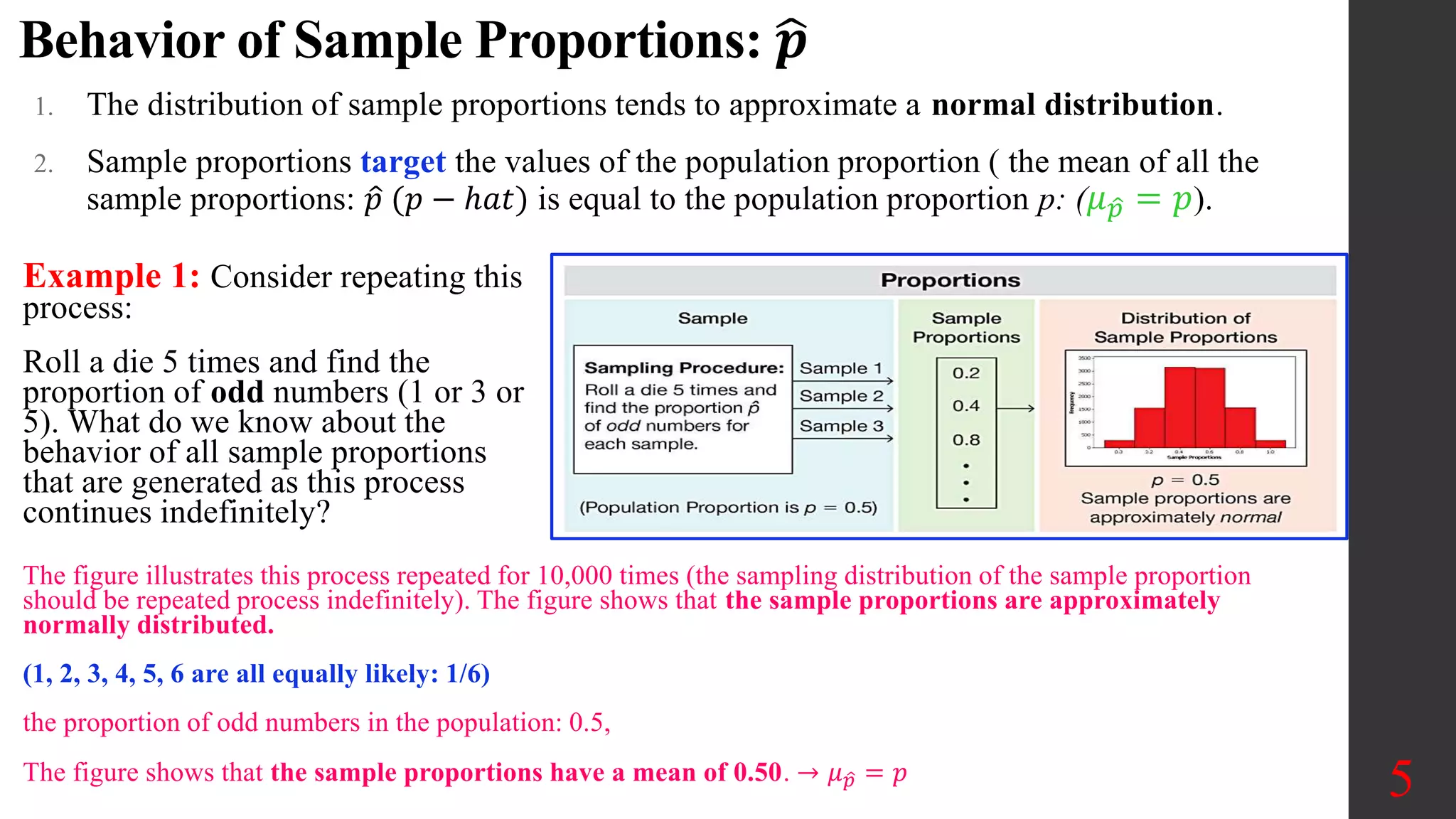
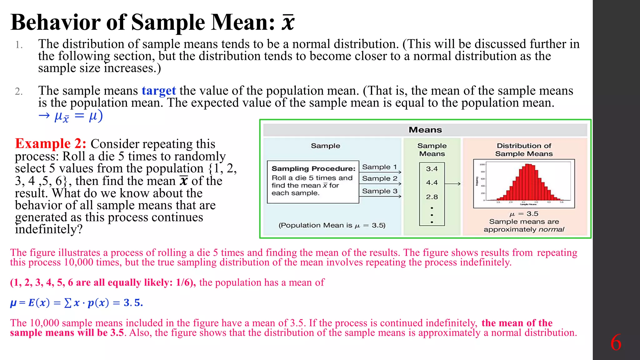
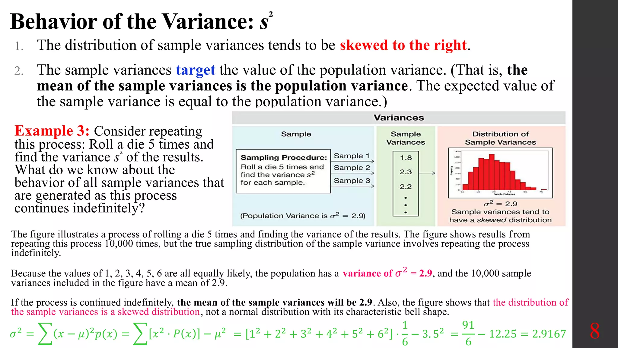
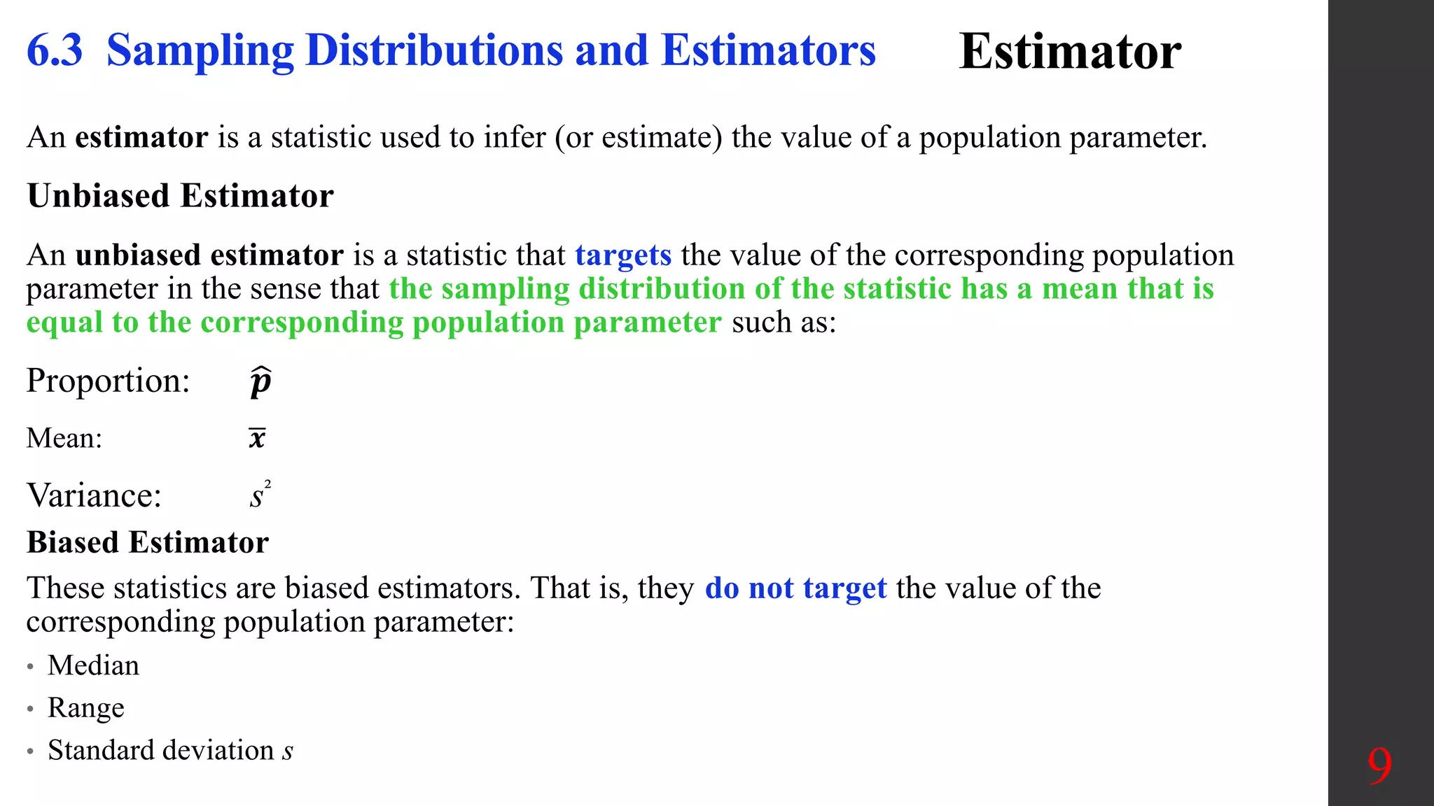
Elementary Statistics
Chapter 6:
Normal Probability
Distribution
6.3 Sampling
Distribution and
Estimators
1
Chapter 6: Normal Probability Distribution
6.1 The Standard Normal Distribution
6.2 Real Applications of Normal Distributions
6.3 Sampling Distributions and Estimators
6.4 The Central Limit Theorem
6.5 Assessing Normality
6.6 Normal as Approximation to Binomial
2
Objectives:
• Identify distributions as symmetric or skewed.
• Identify the properties of a normal distribution.
• Find the area under the standard normal distribution, given various z values.
• Find probabilities for a normally distributed variable by transforming it into a standard normal variable.
• Find specific data values for given percentages, using the standard normal distribution.
• Use the central limit theorem to solve problems involving sample means for large samples.
• Use the normal approximation to compute probabilities for a binomial variable.
Key Concept: In addition to knowing how individual data values vary about the
mean for a population, statisticians are interested in knowing how the means of
samples of the same size taken from the same population vary about the population
mean.
We now consider the concept of a sampling distribution of a statistic. Instead
of working with values from the original population, we want to focus on the
values of statistics (such as sample proportions or sample means) obtained from
the population.
6.3 Sampling Distributions and Estimators
3
Sampling Distribution of a Statistic: The
sampling distribution of a statistic (such as a
sample proportion or sample mean) is the
distribution of all values of the statistic when
all possible samples of the same size n are
taken from the same population. (The
sampling distribution of a statistic is typically
represented as a probability distribution in the
format of a probability histogram, formula, or
table.)
Population proportion: p
Sample proportion: 𝑝 (𝑝 − ℎ𝑎𝑡)
General Behavior of Sampling
Distributions:
1. Sample proportions tend to be normally
distributed.
2. The mean (expected value) of sample
proportions 𝑝 is the same as the population
proportion p. → 𝜇𝑝 = 𝑝
6.3 Sampling Distributions and Estimators
4
Behavior of Sample Proportions: 𝒑
1. The distribution of sample proportions tends to approximate a normal distribution.
2. Sample proportions target the values of the population proportion ( the mean of all the
sample proportions: 𝑝 (𝑝 − ℎ𝑎𝑡) is equal to the population proportion p: (𝜇𝑝 = 𝑝).
5
Example 1: Consider repeating this
process:
Roll a die 5 times and find the
proportion of odd numbers (1 or 3 or
5). What do we know about the
behavior of all sample proportions
that are generated as this process
continues indefinitely?
The figure illustrates this process repeated for 10,000 times (the sampling distribution of the sample proportion
should be repeated process indefinitely). The figure shows that the sample proportions are approximately
normally distributed.
(1, 2, 3, 4, 5, 6 are all equally likely: 1/6)
the proportion of odd numbers in the population: 0.5,
The figure shows that the sample proportions have a mean of 0.50. → 𝜇𝑝 = 𝑝
Behavior of Sample Mean: 𝒙
1. The distribution of sample means tends to be a normal distribution. (This will be discussed further in
the following section, but the distribution tends to become closer to a normal distribution as the
sample size increases.)
2. The sample means target the value of the population mean. (That is, the mean of the sample means
is the population mean. The expected value of the sample mean is equal to the population mean.
→ 𝜇𝑥 = 𝜇)
6
Example 2: Consider repeating this
process: Roll a die 5 times to randomly
select 5 values from the population {1, 2,
3, 4 ,5, 6}, then find the mean 𝒙 of the
result. What do we know about the
behavior of all sample means that are
generated as this process continues
indefinitely?
The figure illustrates a process of rolling a die 5 times and finding the mean of the results. The figure shows results from repeating
this process 10,000 times, but the true sampling distribution of the mean involves repeating the process indefinitely.
(1, 2, 3, 4, 5, 6 are all equally likely: 1/6), the population has a mean of
μ = 𝑬 𝒙 = 𝒙 ∙ 𝒑 𝒙 = 𝟑. 𝟓.
The 10,000 sample means included in the figure have a mean of 3.5. If the process is continued indefinitely, the mean of the
sample means will be 3.5. Also, the figure shows that the distribution of the sample means is approximately a normal distribution.
Sampling Distribution of the Sample Variance
The sampling distribution of the sample variance is the distribution of sample
variances (the variable s²), with all samples having the same sample size n taken from
the same population. (The sampling distribution of the sample variance is typically
represented as a probability distribution in the format of a table, probability histogram,
or formula.)
Behavior of Sample Variances:
1. The distribution of sample variances tends to be a distribution skewed to the right.
2. The sample variances target the value of the population variance. (That is, the
mean of the sample variances is the population variance. The expected value of the
sample variance is equal to the population variance.) 𝜇𝑠2 = 𝜎2
7
Population standard deviation:
Population variance:
𝜎2
=
𝑥 − 𝜇 2
𝑁 𝜎 =
𝑥 − 𝜇 2
𝑁
Behavior of the Variance: s²
1. The distribution of sample variances tends to be skewed to the right.
2. The sample variances target the value of the population variance. (That is, the
mean of the sample variances is the population variance. The expected value of
the sample variance is equal to the population variance.)
8
Example 3: Consider repeating
this process: Roll a die 5 times and
find the variance s² of the results.
What do we know about the
behavior of all sample variances that
are generated as this process
continues indefinitely?
The figure illustrates a process of rolling a die 5 times and finding the variance of the results. The figure shows results from
repeating this process 10,000 times, but the true sampling distribution of the sample variance involves repeating the process
indefinitely.
Because the values of 1, 2, 3, 4, 5, 6 are all equally likely, the population has a variance of 𝜎2
= 2.9, and the 10,000 sample
variances included in the figure have a mean of 2.9.
If the process is continued indefinitely, the mean of the sample variances will be 2.9. Also, the figure shows that the distribution of
the sample variances is a skewed distribution, not a normal distribution with its characteristic bell shape.
𝜎2
= 𝑥 − 𝜇 2
𝑝(𝑥) = 𝑥2
⋅ 𝑃 𝑥 − 𝜇2
= 12 + 22 + 32 + 42 + 52 + 62 ⋅
1
6
− 3. 52 =
91
6
− 12.25 = 2.9167
Estimator
An estimator is a statistic used to infer (or estimate) the value of a population parameter.
Unbiased Estimator
An unbiased estimator is a statistic that targets the value of the corresponding population
parameter in the sense that the sampling distribution of the statistic has a mean that is
equal to the corresponding population parameter such as:
Proportion: 𝒑
Mean: 𝒙
Variance: s²
Biased Estimator
These statistics are biased estimators. That is, they do not target the value of the
corresponding population parameter:
• Median
• Range
• Standard deviation s
9
6.3 Sampling Distributions and Estimators
Why Sample with Replacement?
1. When selecting a relatively small sample from a large population, it makes no
significant difference whether we sample with replacement or without
replacement.
2. Sampling with replacement results in independent events that are unaffected by
previous outcomes, and independent events are easier to analyze and result in
simpler calculations and formulas.
10

Sampling Distributions and Estimators

  • 1.
    Elementary Statistics Chapter 6: NormalProbability Distribution 6.3 Sampling Distribution and Estimators 1
  • 2.
    Chapter 6: NormalProbability Distribution 6.1 The Standard Normal Distribution 6.2 Real Applications of Normal Distributions 6.3 Sampling Distributions and Estimators 6.4 The Central Limit Theorem 6.5 Assessing Normality 6.6 Normal as Approximation to Binomial 2 Objectives: • Identify distributions as symmetric or skewed. • Identify the properties of a normal distribution. • Find the area under the standard normal distribution, given various z values. • Find probabilities for a normally distributed variable by transforming it into a standard normal variable. • Find specific data values for given percentages, using the standard normal distribution. • Use the central limit theorem to solve problems involving sample means for large samples. • Use the normal approximation to compute probabilities for a binomial variable.
  • 3.
    Key Concept: Inaddition to knowing how individual data values vary about the mean for a population, statisticians are interested in knowing how the means of samples of the same size taken from the same population vary about the population mean. We now consider the concept of a sampling distribution of a statistic. Instead of working with values from the original population, we want to focus on the values of statistics (such as sample proportions or sample means) obtained from the population. 6.3 Sampling Distributions and Estimators 3
  • 4.
    Sampling Distribution ofa Statistic: The sampling distribution of a statistic (such as a sample proportion or sample mean) is the distribution of all values of the statistic when all possible samples of the same size n are taken from the same population. (The sampling distribution of a statistic is typically represented as a probability distribution in the format of a probability histogram, formula, or table.) Population proportion: p Sample proportion: 𝑝 (𝑝 − ℎ𝑎𝑡) General Behavior of Sampling Distributions: 1. Sample proportions tend to be normally distributed. 2. The mean (expected value) of sample proportions 𝑝 is the same as the population proportion p. → 𝜇𝑝 = 𝑝 6.3 Sampling Distributions and Estimators 4
  • 5.
    Behavior of SampleProportions: 𝒑 1. The distribution of sample proportions tends to approximate a normal distribution. 2. Sample proportions target the values of the population proportion ( the mean of all the sample proportions: 𝑝 (𝑝 − ℎ𝑎𝑡) is equal to the population proportion p: (𝜇𝑝 = 𝑝). 5 Example 1: Consider repeating this process: Roll a die 5 times and find the proportion of odd numbers (1 or 3 or 5). What do we know about the behavior of all sample proportions that are generated as this process continues indefinitely? The figure illustrates this process repeated for 10,000 times (the sampling distribution of the sample proportion should be repeated process indefinitely). The figure shows that the sample proportions are approximately normally distributed. (1, 2, 3, 4, 5, 6 are all equally likely: 1/6) the proportion of odd numbers in the population: 0.5, The figure shows that the sample proportions have a mean of 0.50. → 𝜇𝑝 = 𝑝
  • 6.
    Behavior of SampleMean: 𝒙 1. The distribution of sample means tends to be a normal distribution. (This will be discussed further in the following section, but the distribution tends to become closer to a normal distribution as the sample size increases.) 2. The sample means target the value of the population mean. (That is, the mean of the sample means is the population mean. The expected value of the sample mean is equal to the population mean. → 𝜇𝑥 = 𝜇) 6 Example 2: Consider repeating this process: Roll a die 5 times to randomly select 5 values from the population {1, 2, 3, 4 ,5, 6}, then find the mean 𝒙 of the result. What do we know about the behavior of all sample means that are generated as this process continues indefinitely? The figure illustrates a process of rolling a die 5 times and finding the mean of the results. The figure shows results from repeating this process 10,000 times, but the true sampling distribution of the mean involves repeating the process indefinitely. (1, 2, 3, 4, 5, 6 are all equally likely: 1/6), the population has a mean of μ = 𝑬 𝒙 = 𝒙 ∙ 𝒑 𝒙 = 𝟑. 𝟓. The 10,000 sample means included in the figure have a mean of 3.5. If the process is continued indefinitely, the mean of the sample means will be 3.5. Also, the figure shows that the distribution of the sample means is approximately a normal distribution.
  • 7.
    Sampling Distribution ofthe Sample Variance The sampling distribution of the sample variance is the distribution of sample variances (the variable s²), with all samples having the same sample size n taken from the same population. (The sampling distribution of the sample variance is typically represented as a probability distribution in the format of a table, probability histogram, or formula.) Behavior of Sample Variances: 1. The distribution of sample variances tends to be a distribution skewed to the right. 2. The sample variances target the value of the population variance. (That is, the mean of the sample variances is the population variance. The expected value of the sample variance is equal to the population variance.) 𝜇𝑠2 = 𝜎2 7 Population standard deviation: Population variance: 𝜎2 = 𝑥 − 𝜇 2 𝑁 𝜎 = 𝑥 − 𝜇 2 𝑁
  • 8.
    Behavior of theVariance: s² 1. The distribution of sample variances tends to be skewed to the right. 2. The sample variances target the value of the population variance. (That is, the mean of the sample variances is the population variance. The expected value of the sample variance is equal to the population variance.) 8 Example 3: Consider repeating this process: Roll a die 5 times and find the variance s² of the results. What do we know about the behavior of all sample variances that are generated as this process continues indefinitely? The figure illustrates a process of rolling a die 5 times and finding the variance of the results. The figure shows results from repeating this process 10,000 times, but the true sampling distribution of the sample variance involves repeating the process indefinitely. Because the values of 1, 2, 3, 4, 5, 6 are all equally likely, the population has a variance of 𝜎2 = 2.9, and the 10,000 sample variances included in the figure have a mean of 2.9. If the process is continued indefinitely, the mean of the sample variances will be 2.9. Also, the figure shows that the distribution of the sample variances is a skewed distribution, not a normal distribution with its characteristic bell shape. 𝜎2 = 𝑥 − 𝜇 2 𝑝(𝑥) = 𝑥2 ⋅ 𝑃 𝑥 − 𝜇2 = 12 + 22 + 32 + 42 + 52 + 62 ⋅ 1 6 − 3. 52 = 91 6 − 12.25 = 2.9167
  • 9.
    Estimator An estimator isa statistic used to infer (or estimate) the value of a population parameter. Unbiased Estimator An unbiased estimator is a statistic that targets the value of the corresponding population parameter in the sense that the sampling distribution of the statistic has a mean that is equal to the corresponding population parameter such as: Proportion: 𝒑 Mean: 𝒙 Variance: s² Biased Estimator These statistics are biased estimators. That is, they do not target the value of the corresponding population parameter: • Median • Range • Standard deviation s 9 6.3 Sampling Distributions and Estimators
  • 10.
    Why Sample withReplacement? 1. When selecting a relatively small sample from a large population, it makes no significant difference whether we sample with replacement or without replacement. 2. Sampling with replacement results in independent events that are unaffected by previous outcomes, and independent events are easier to analyze and result in simpler calculations and formulas. 10