Vibrant technologies & computers
Vashi
Vibranttechnologies.co.in
vibrant technologies & computer
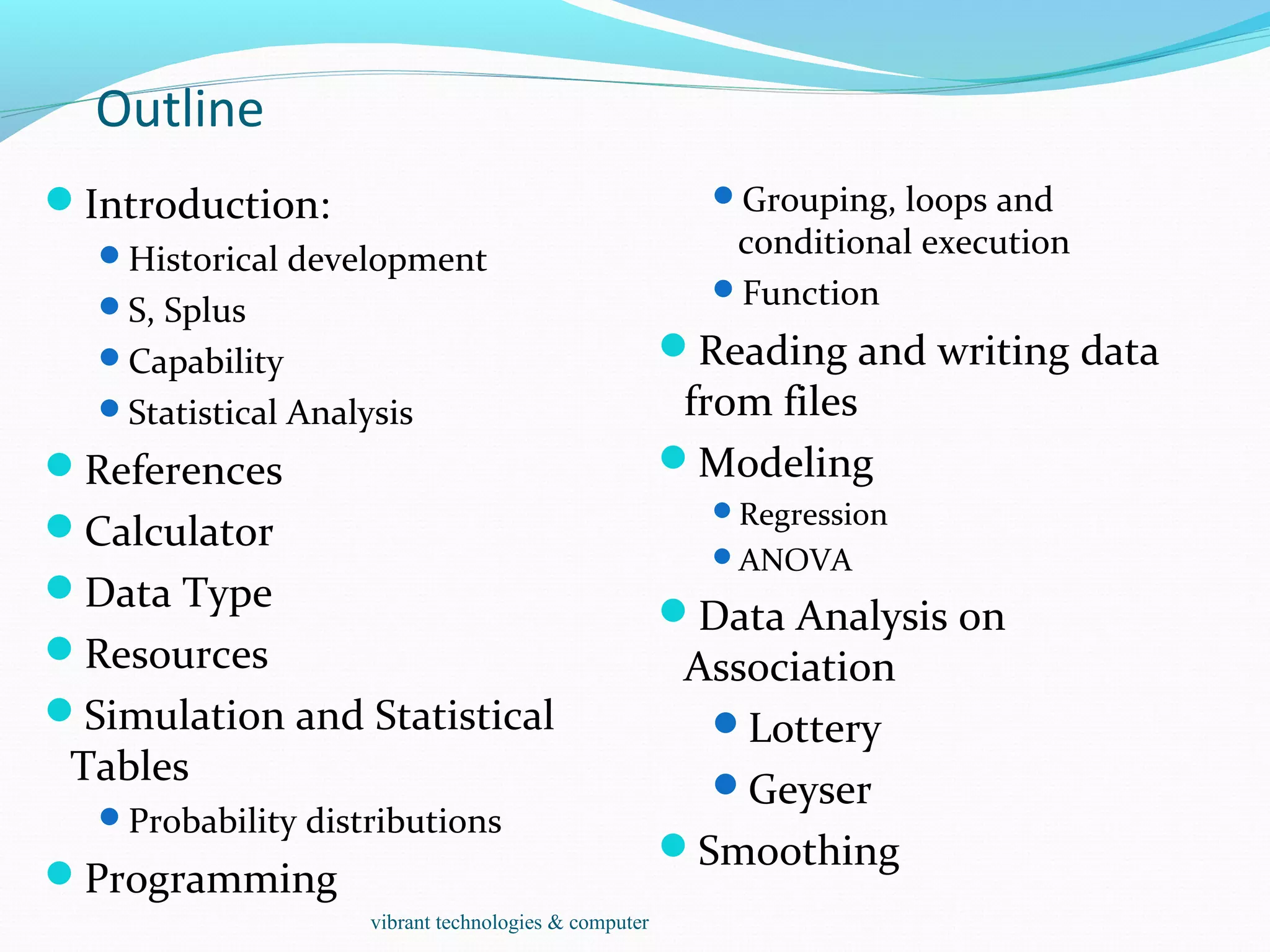
Outline
Introduction:
Historical development
S, Splus
Capability
Statistical Analysis
References
Calculator
Data Type
Resources
Simulation and Statistical
Tables
Probability distributions
Programming
Grouping, loops and
conditional execution
Function
Reading and writing data
from files
Modeling
Regression
ANOVA
Data Analysis on
Association
Lottery
Geyser
Smoothing
vibrant technologies & computer
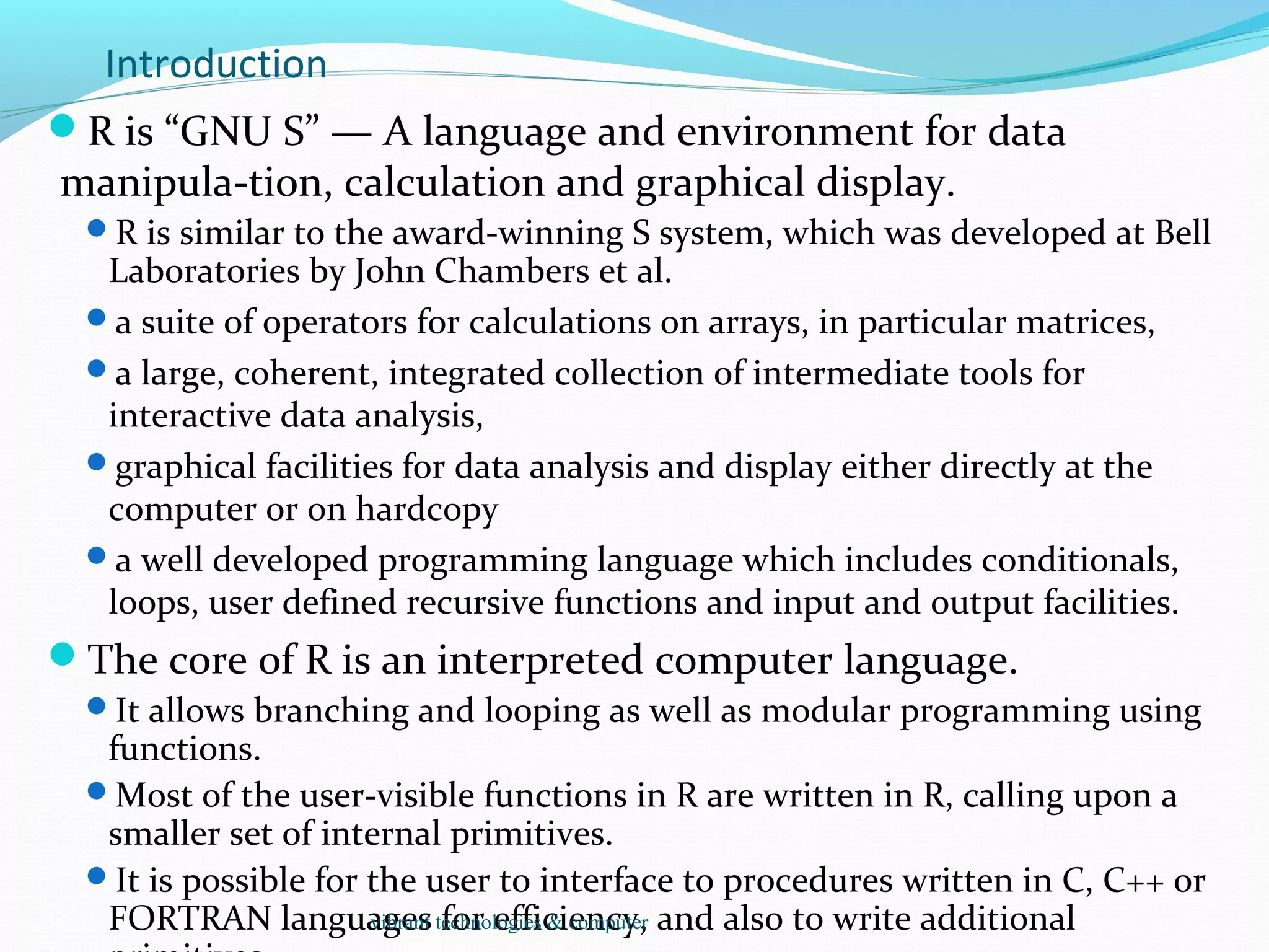
Introduction
R is “GNU S” — A language and environment for data
manipula-tion, calculation and graphical display.
R is similar to the award-winning S system, which was developed at Bell
Laboratories by John Chambers et al.
a suite of operators for calculations on arrays, in particular matrices,
a large, coherent, integrated collection of intermediate tools for
interactive data analysis,
graphical facilities for data analysis and display either directly at the
computer or on hardcopy
a well developed programming language which includes conditionals,
loops, user defined recursive functions and input and output facilities.
The core of R is an interpreted computer language.
It allows branching and looping as well as modular programming using
functions.
Most of the user-visible functions in R are written in R, calling upon a
smaller set of internal primitives.
It is possible for the user to interface to procedures written in C, C++ or
FORTRAN languages for efficiency, and also to write additionalvibrant technologies & computer
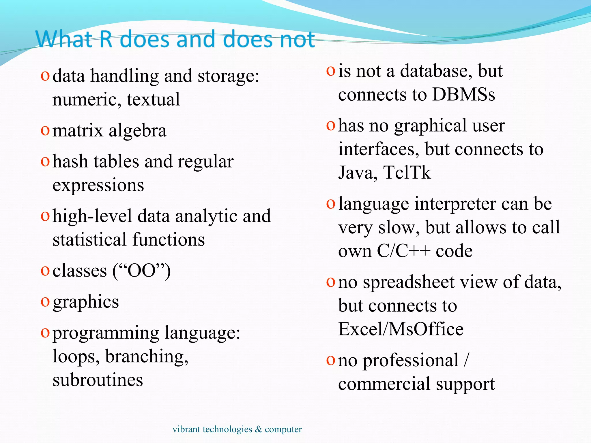
odata handling and storage:
numeric, textual
omatrix algebra
ohash tables and regular
expressions
ohigh-level data analytic and
statistical functions
oclasses (“OO”)
ographics
oprogramming language:
loops, branching,
subroutines
ois not a database, but
connects to DBMSs
ohas no graphical user
interfaces, but connects to
Java, TclTk
olanguage interpreter can be
very slow, but allows to call
own C/C++ code
ono spreadsheet view of data,
but connects to
Excel/MsOffice
ono professional /
commercial support
vibrant technologies & computer
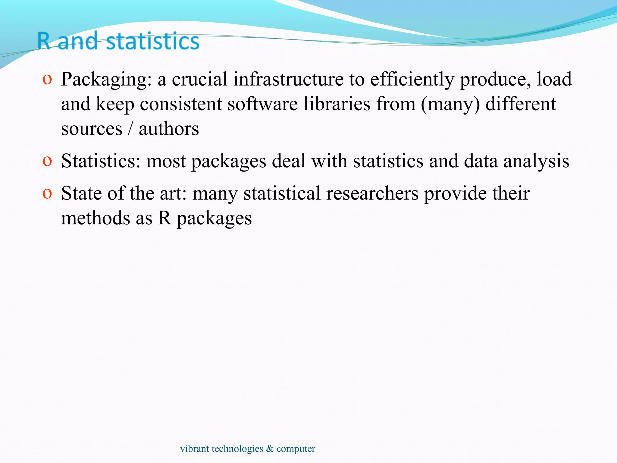
o Packaging: a crucial infrastructure to efficiently produce, load
and keep consistent software libraries from (many) different
sources / authors
o Statistics: most packages deal with statistics and data analysis
o State of the art: many statistical researchers provide their
methods as R packages
vibrant technologies & computer
Data Analysis and Presentation
The R distribution contains functionality for large number of
statistical procedures.
linear and generalized linear models
nonlinear regression models
time series analysis
classical parametric and nonparametric tests
clustering
smoothing
R also has a large set of functions which provide a flexible
graphical environment for creating various kinds of data
presentations.
vibrant technologies & computer
References
For R,
The basic reference is The New S Language: A Programming
Environment for Data Analysis and Graphics by Richard A. Becker,
John M. Chambers and Allan R. Wilks (the “Blue Book”) .
The new features of the 1991 release of S (S version 3) are covered in
Statistical Models in S edited by John M. Chambers and Trevor J.
Hastie (the “White Book”).
Classical and modern statistical techniques have been implemented.
 Some of these are built into the base R environment.
 Many are supplied as packages. There are about 8 packages supplied with
R (called “standard” packages) and many more are available through the
cran family of Internet sites (via http://cran.r-project.org).
All the R functions have been documented in the form of
help pages in an “output independent” form which can be
used to create versions for HTML, LATEX, text etc.
The document “An Introduction to R” provides a more user-friendly
starting point.
An “R Language Definition” manual
More specialized manuals on data import/export and extending R.
vibrant technologies & computer
> log2(32)
[1] 5
> sqrt(2)
[1] 1.414214
> seq(0, 5, length=6)
[1] 0 1 2 3 4 5
> plot(sin(seq(0, 2*pi, length=100)))
0 20 40 60 80 100
-1.0-0.50.00.51.0
Index
sin(seq(0,2*pi,length=100))
vibrant technologies & computer
primitive (or: atomic) data types in R are:
• numeric (integer, double, complex)
• character
• logical
• function
out of these, vectors, arrays, lists can be built.
vibrant technologies & computer
• Object: a collection of atomic variables and/or other objects that
belong together
• Example: a microarray experiment
• probe intensities
• patient data (tissue location, diagnosis, follow-up)
• gene data (sequence, IDs, annotation)
Parlance:
• class: the “abstract” definition of it
• object: a concrete instance
• method: other word for ‘function’
• slot: a component of an object
vibrant technologies & computer
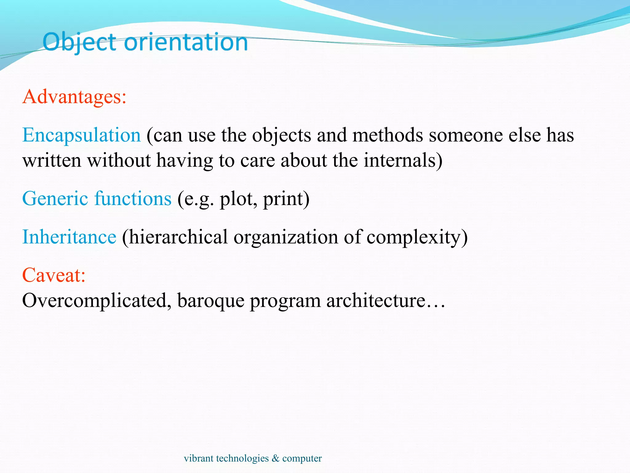
Advantages:
Encapsulation (can use the objects and methods someone else has
written without having to care about the internals)
Generic functions (e.g. plot, print)
Inheritance (hierarchical organization of complexity)
Caveat:
Overcomplicated, baroque program architecture…
vibrant technologies & computer
> a = 49
> sqrt(a)
[1] 7
> a = "The dog ate my homework"
> sub("dog","cat",a)
[1] "The cat ate my homework“
> a = (1+1==3)
> a
[1] FALSE
numeric
character
string
logical
vibrant technologies & computer
• vector: an ordered collection of data of the same type
> a = c(1,2,3)
> a*2
[1] 2 4 6
• Example: the mean spot intensities of all 15488 spots on a chip:
a vector of 15488 numbers
• In R, a single number is the special case of a vector with 1
element.
• Other vector types: character strings, logical
vibrant technologies & computer
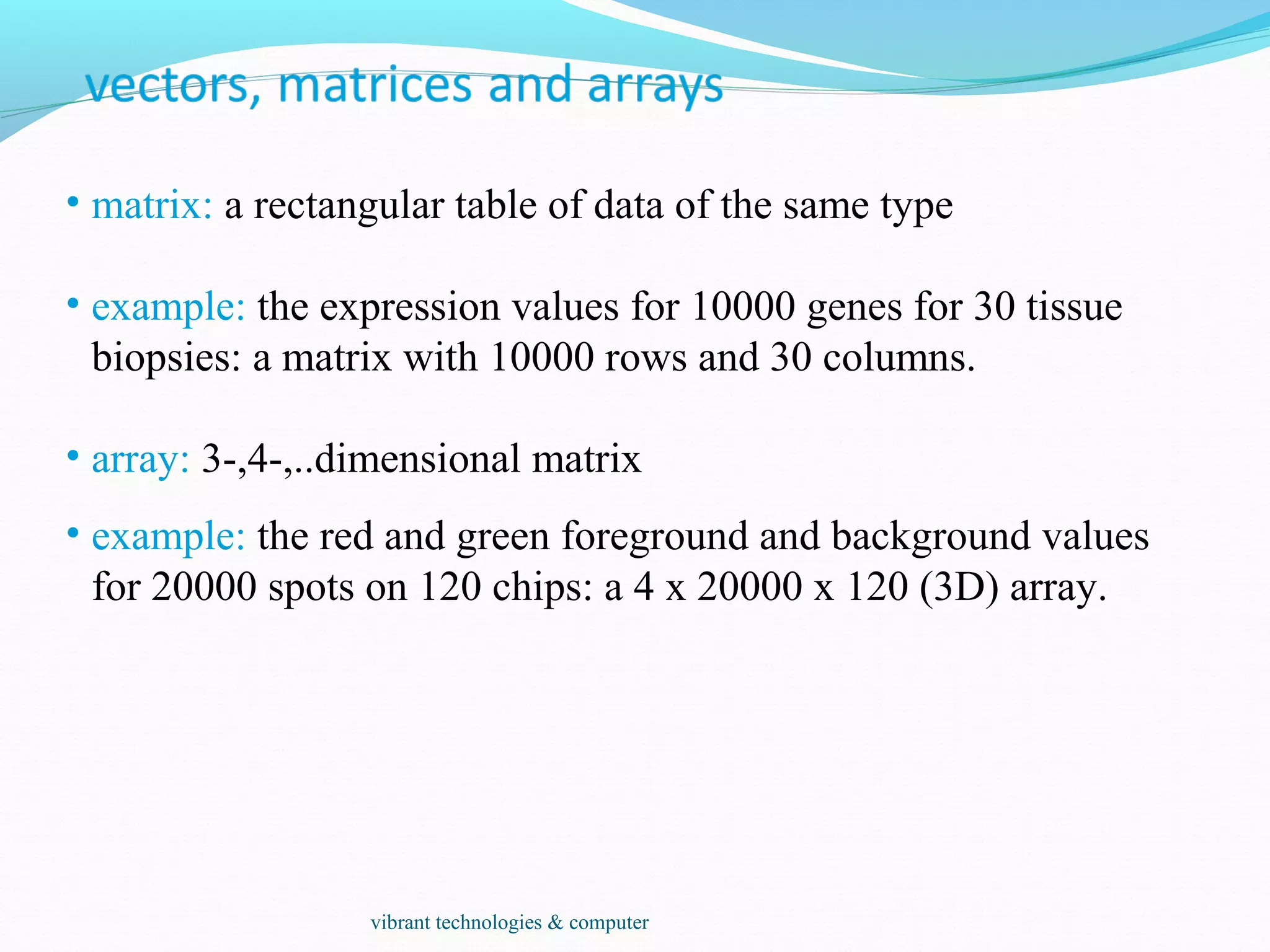
• matrix: a rectangular table of data of the same type
• example: the expression values for 10000 genes for 30 tissue
biopsies: a matrix with 10000 rows and 30 columns.
• array: 3-,4-,..dimensional matrix
• example: the red and green foreground and background values
for 20000 spots on 120 chips: a 4 x 20000 x 120 (3D) array.
vibrant technologies & computer
• vector: an ordered collection of data of the same type.
> a = c(7,5,1)
> a[2]
[1] 5
• list: an ordered collection of data of arbitrary types.
> doe = list(name="john",age=28,married=F)
> doe$name
[1] "john“
> doe$age
[1] 28
• Typically, vector elements are accessed by their index (an integer),
list elements by their name (a character string). But both types
support both access methods.
vibrant technologies & computer
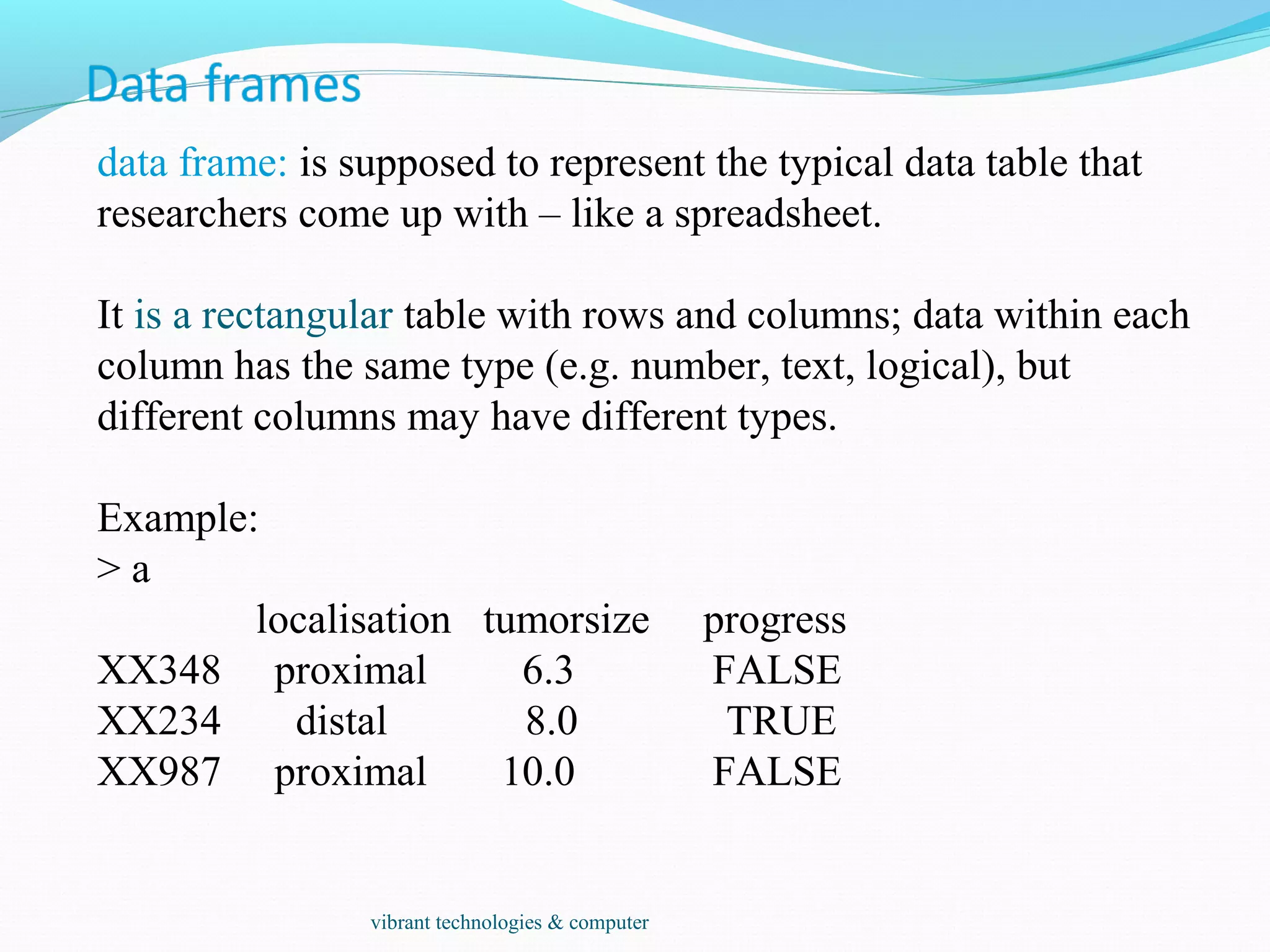
data frame: is supposed to represent the typical data table that
researchers come up with – like a spreadsheet.
It is a rectangular table with rows and columns; data within each
column has the same type (e.g. number, text, logical), but
different columns may have different types.
Example:
> a
localisation tumorsize progress
XX348 proximal 6.3 FALSE
XX234 distal 8.0 TRUE
XX987 proximal 10.0 FALSE
vibrant technologies & computer
A character string can contain arbitrary text. Sometimes it is useful to use a limited
vocabulary, with a small number of allowed words. A factor is a variable that can only
take such a limited number of values, which are called levels.
> a
[1] Kolon(Rektum) Magen Magen
[4] Magen Magen Retroperitoneal
[7] Magen Magen(retrogastral) Magen
Levels: Kolon(Rektum) Magen Magen(retrogastral) Retroperitoneal
> class(a)
[1] "factor"
> as.character(a)
[1] "Kolon(Rektum)" "Magen" "Magen"
[4] "Magen" "Magen" "Retroperitoneal"
[7] "Magen" "Magen(retrogastral)" "Magen"
> as.integer(a)
[1] 1 2 2 2 2 4 2 3 2
> as.integer(as.character(a))
[1] NA NA NA NA NA NA NA NA NA NA NA NA
Warning message: NAs introduced by coercion
vibrant technologies & computer
Individual elements of a vector, matrix, array or data frame are
accessed with “[ ]” by specifying their index, or their name
> a
localisation tumorsize progress
XX348 proximal 6.3 0
XX234 distal 8.0 1
XX987 proximal 10.0 0
> a[3, 2]
[1] 10
> a["XX987", "tumorsize"]
[1] 10
> a["XX987",]
localisation tumorsize progress
XX987 proximal 10 0
vibrant technologies & computer
> a
localisation tumorsize progress
XX348 proximal 6.3 0
XX234 distal 8.0 1
XX987 proximal 10.0 0
> a[c(1,3),]
localisation tumorsize progress
XX348 proximal 6.3 0
XX987 proximal 10.0 0
> a[c(T,F,T),]
localisation tumorsize progress
XX348 proximal 6.3 0
XX987 proximal 10.0 0
> a$localisation
[1] "proximal" "distal" "proximal"
> a$localisation=="proximal"
[1] TRUE FALSE TRUE
> a[ a$localisation=="proximal", ]
localisation tumorsize progress
XX348 proximal 6.3 0
XX987 proximal 10.0 0
subset rows by a
vector of indices
subset rows by a
logical vector
subset a column
comparison resulting in
logical vector
subset the selected
rows
vibrant technologies & computer
Resources
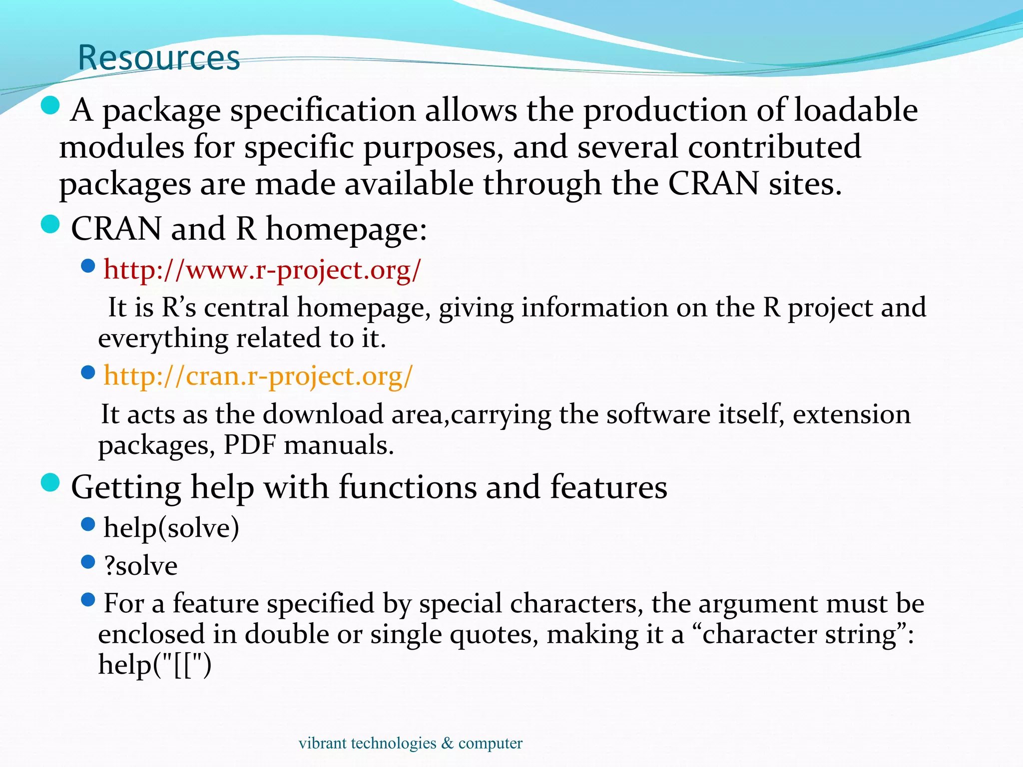
A package specification allows the production of loadable
modules for specific purposes, and several contributed
packages are made available through the CRAN sites.
CRAN and R homepage:
http://www.r-project.org/
It is R’s central homepage, giving information on the R project and
everything related to it.
http://cran.r-project.org/
It acts as the download area,carrying the software itself, extension
packages, PDF manuals.
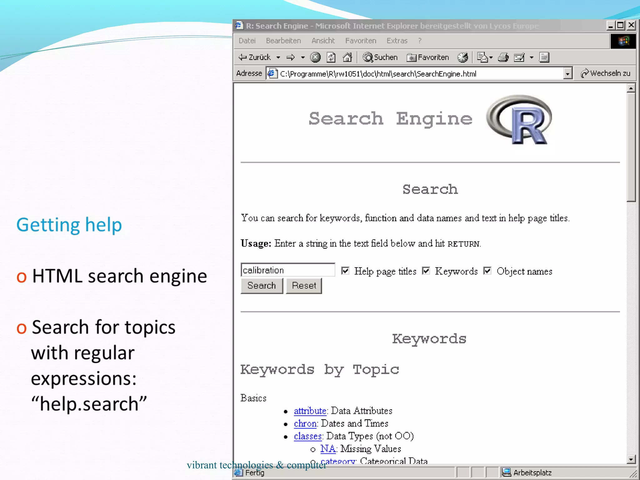
Getting help with functions and features
help(solve)
?solve
For a feature specified by special characters, the argument must be
enclosed in double or single quotes, making it a “character string”:
help("[[")
vibrant technologies & computer
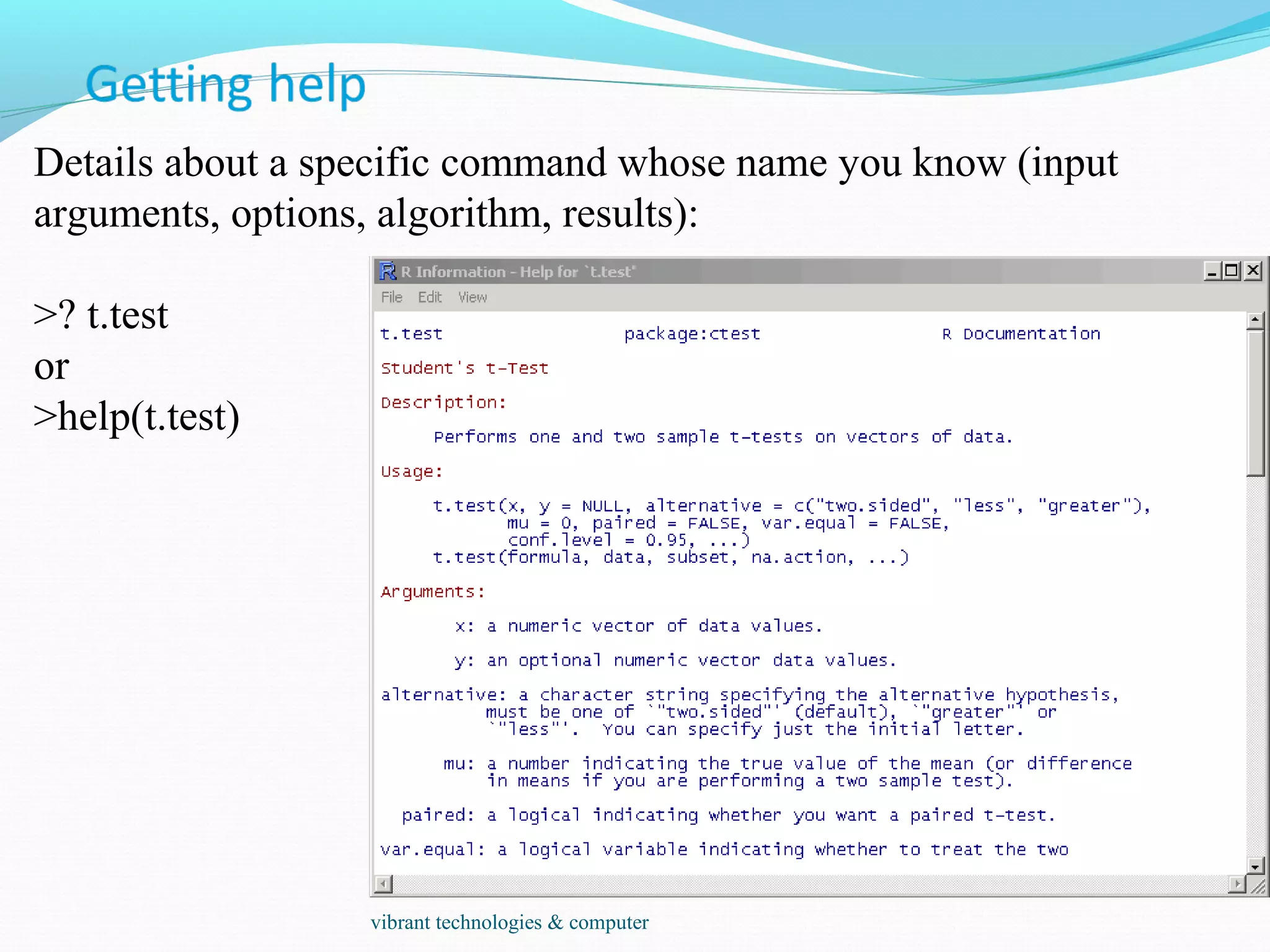
Details about a specific command whose name you know (input
arguments, options, algorithm, results):
>? t.test
or
>help(t.test)
vibrant technologies & computer
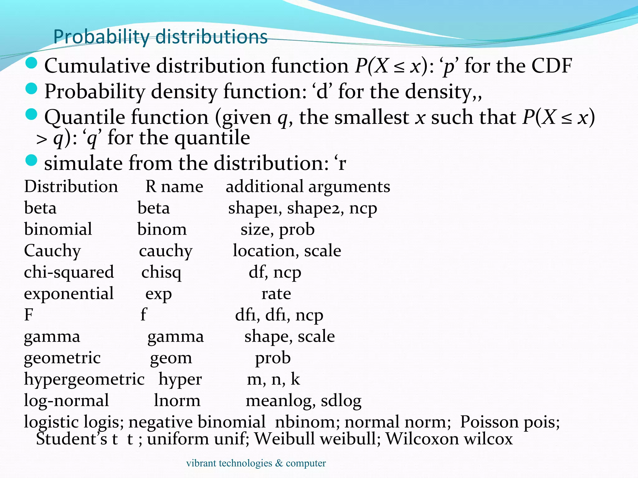
Probability distributions
Cumulative distribution function P(X ≤ x): ‘p’ for the CDF
Probability density function: ‘d’ for the density,,
Quantile function (given q, the smallest x such that P(X ≤ x)
> q): ‘q’ for the quantile
simulate from the distribution: ‘r
Distribution R name additional arguments
beta beta shape1, shape2, ncp
binomial binom size, prob
Cauchy cauchy location, scale
chi-squared chisq df, ncp
exponential exp rate
F f df1, df1, ncp
gamma gamma shape, scale
geometric geom prob
hypergeometric hyper m, n, k
log-normal lnorm meanlog, sdlog
logistic logis; negative binomial nbinom; normal norm; Poisson pois;
Student’s t t ; uniform unif; Weibull weibull; Wilcoxon wilcox
vibrant technologies & computer
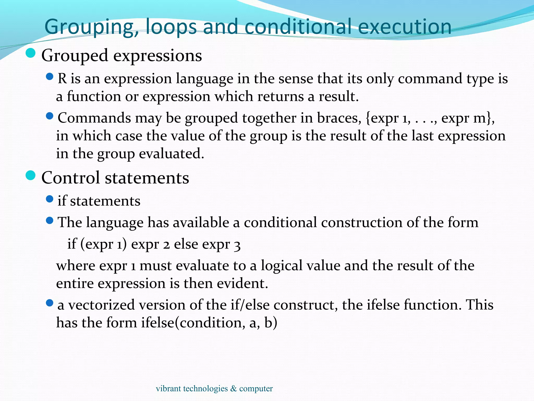
Grouping, loops and conditional execution
Grouped expressions
R is an expression language in the sense that its only command type is
a function or expression which returns a result.
Commands may be grouped together in braces, {expr 1, . . ., expr m},
in which case the value of the group is the result of the last expression
in the group evaluated.
Control statements
if statements
The language has available a conditional construction of the form
if (expr 1) expr 2 else expr 3
where expr 1 must evaluate to a logical value and the result of the
entire expression is then evident.
a vectorized version of the if/else construct, the ifelse function. This
has the form ifelse(condition, a, b)
vibrant technologies & computer
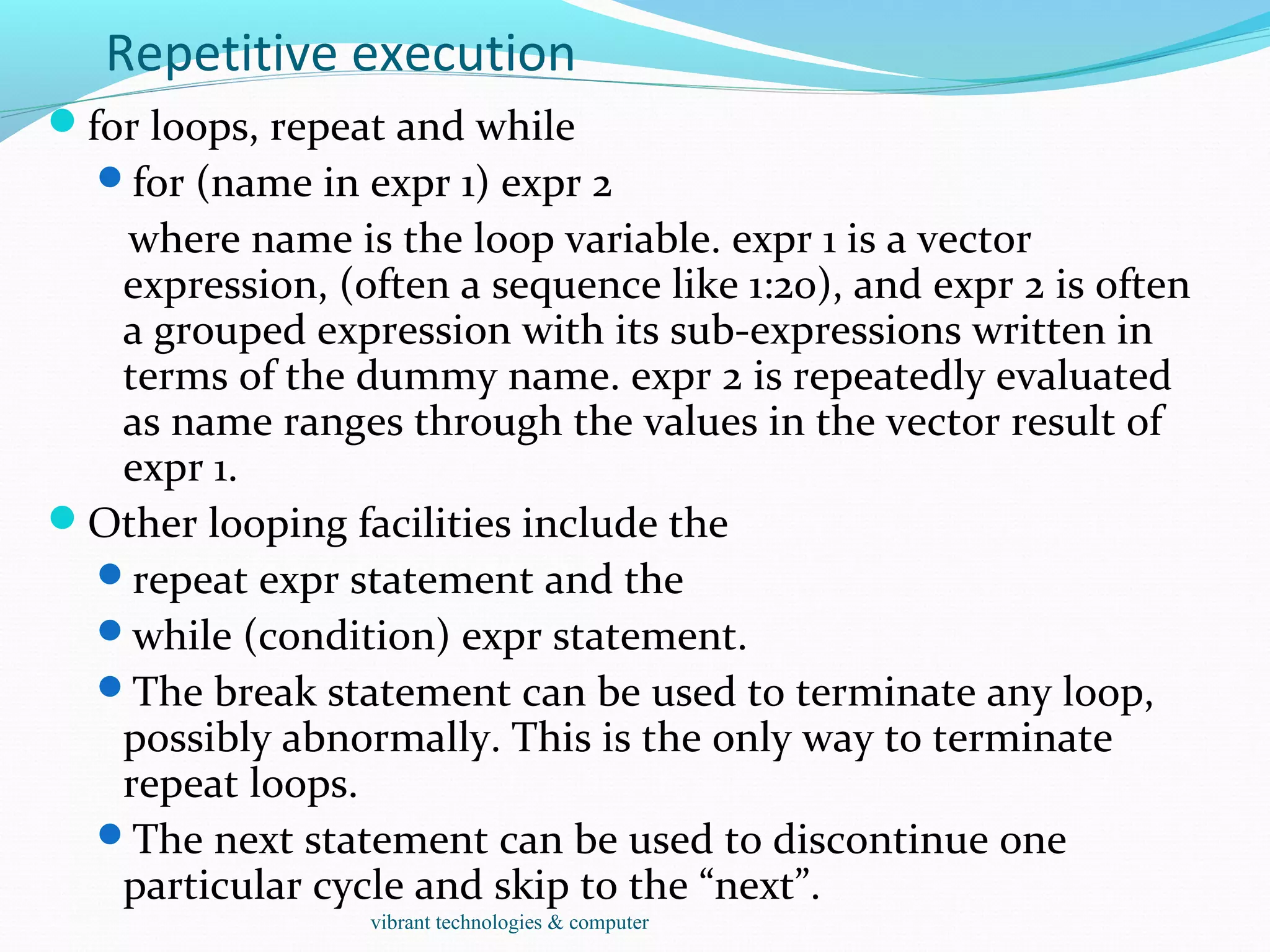
Repetitive execution
for loops, repeat and while
for (name in expr 1) expr 2
where name is the loop variable. expr 1 is a vector
expression, (often a sequence like 1:20), and expr 2 is often
a grouped expression with its sub-expressions written in
terms of the dummy name. expr 2 is repeatedly evaluated
as name ranges through the values in the vector result of
expr 1.
Other looping facilities include the
repeat expr statement and the
while (condition) expr statement.
The break statement can be used to terminate any loop,
possibly abnormally. This is the only way to terminate
repeat loops.
The next statement can be used to discontinue one
particular cycle and skip to the “next”.
vibrant technologies & computer
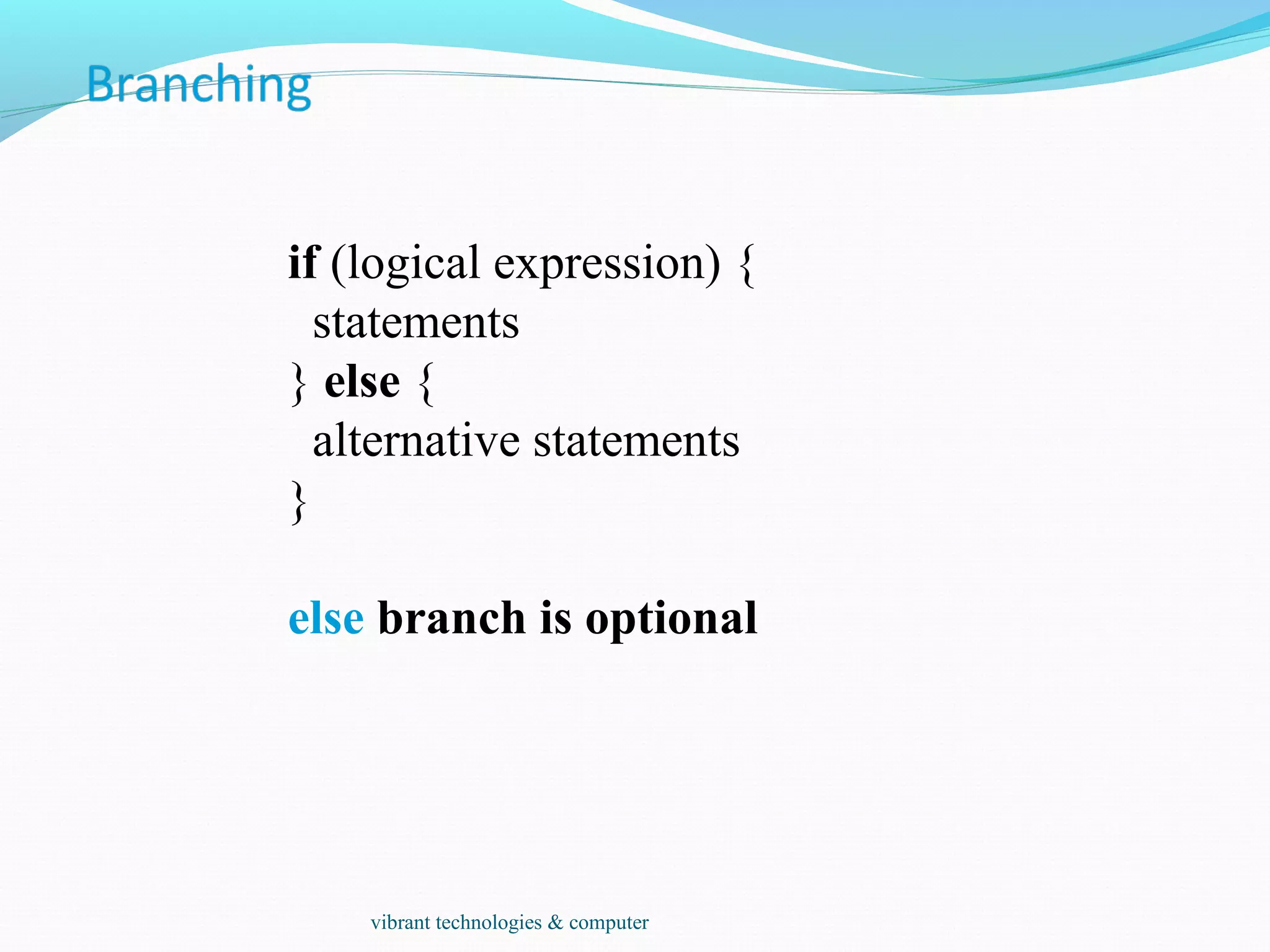
if (logical expression) {
statements
} else {
alternative statements
}
else branch is optional
vibrant technologies & computer
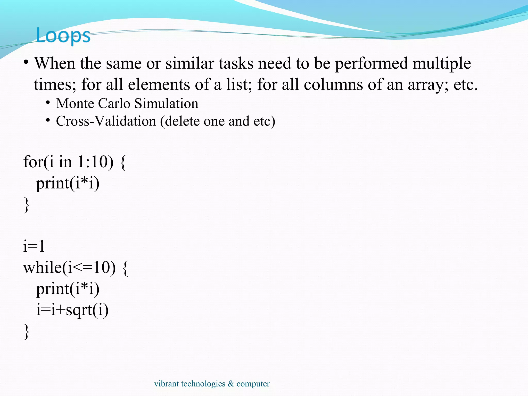
• When the same or similar tasks need to be performed multiple
times; for all elements of a list; for all columns of an array; etc.
• Monte Carlo Simulation
• Cross-Validation (delete one and etc)
for(i in 1:10) {
print(i*i)
}
i=1
while(i<=10) {
print(i*i)
i=i+sqrt(i)
}
vibrant technologies & computer
• When the same or similar tasks need to be performed multiple
times for all elements of a list or for all columns of an array.
• May be easier and faster than “for” loops
• lapply(li, function )
• To each element of the list li, the function function is applied.
• The result is a list whose elements are the individual function
results.
> li = list("klaus","martin","georg")
> lapply(li, toupper)
> [[1]]
> [1] "KLAUS"
> [[2]]
> [1] "MARTIN"
> [[3]]
> [1] "GEORG"
vibrant technologies & computer
sapply( li, fct )
Like apply, but tries to simplify the result, by converting it into a
vector or array of appropriate size
> li = list("klaus","martin","georg")
> sapply(li, toupper)
[1] "KLAUS" "MARTIN" "GEORG"
> fct = function(x) { return(c(x, x*x, x*x*x)) }
> sapply(1:5, fct)
[,1] [,2] [,3] [,4] [,5]
[1,] 1 2 3 4 5
[2,] 1 4 9 16 25
[3,] 1 8 27 64 125
vibrant technologies & computer
apply( arr, margin, fct )
Apply the function fct along some dimensions of the array arr,
according to margin, and return a vector or array of the
appropriate size.
> x
[,1] [,2] [,3]
[1,] 5 7 0
[2,] 7 9 8
[3,] 4 6 7
[4,] 6 3 5
> apply(x, 1, sum)
[1] 12 24 17 14
> apply(x, 2, sum)
[1] 22 25 20
vibrant technologies & computer
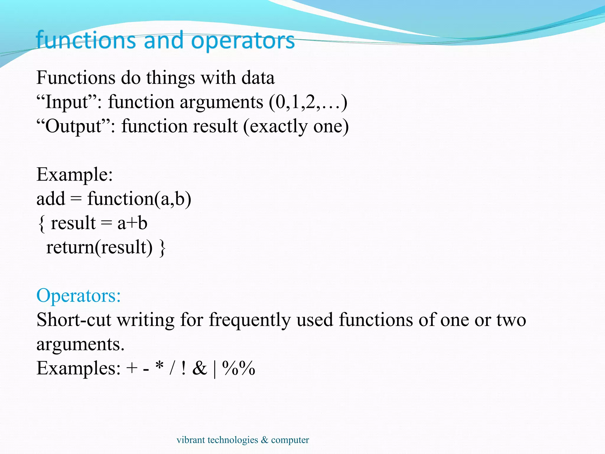
Functions do things with data
“Input”: function arguments (0,1,2,…)
“Output”: function result (exactly one)
Example:
add = function(a,b)
{ result = a+b
return(result) }
Operators:
Short-cut writing for frequently used functions of one or two
arguments.
Examples: + - * / ! & | %%
vibrant technologies & computer
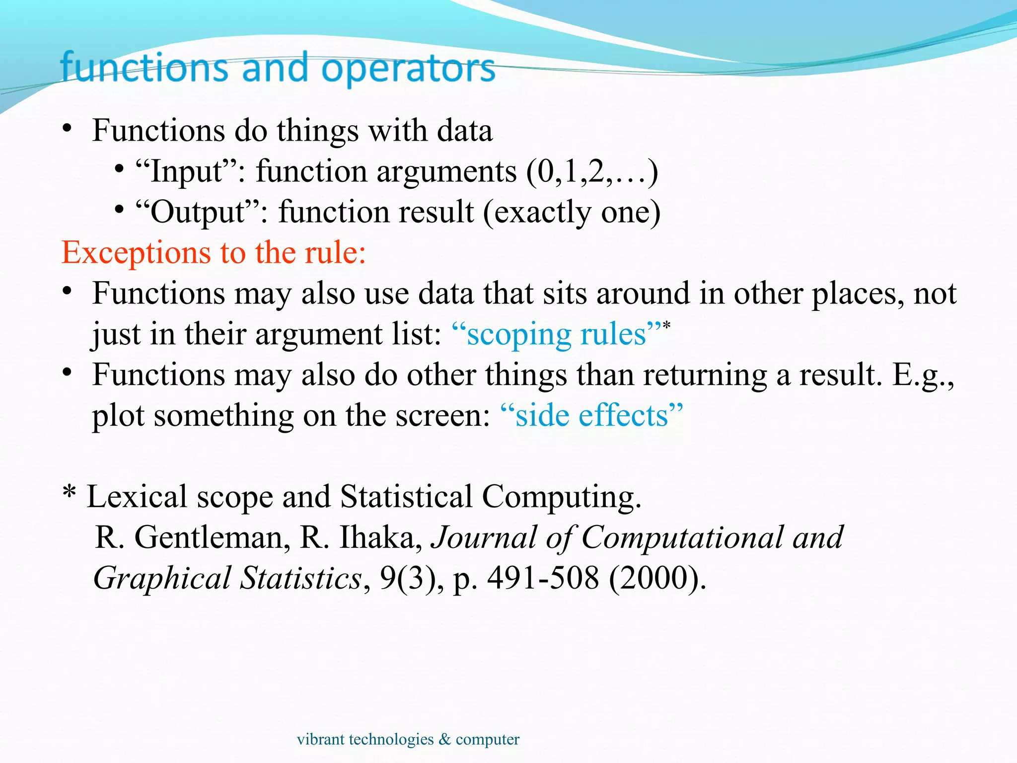
• Functions do things with data
• “Input”: function arguments (0,1,2,…)
• “Output”: function result (exactly one)
Exceptions to the rule:
• Functions may also use data that sits around in other places, not
just in their argument list: “scoping rules”*
• Functions may also do other things than returning a result. E.g.,
plot something on the screen: “side effects”
* Lexical scope and Statistical Computing.
R. Gentleman, R. Ihaka, Journal of Computational and
Graphical Statistics, 9(3), p. 491-508 (2000).
vibrant technologies & computer
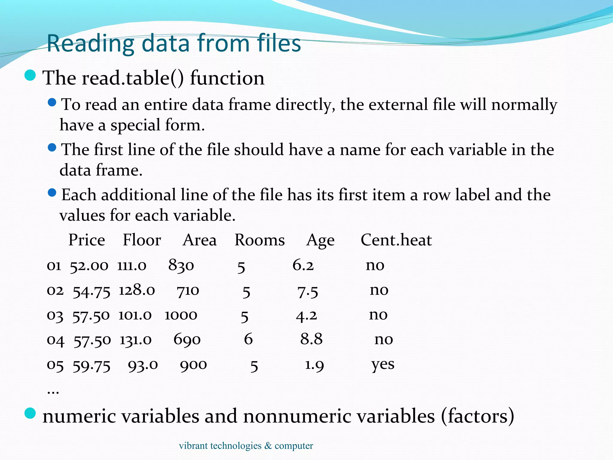
Reading data from files
The read.table() function
To read an entire data frame directly, the external file will normally
have a special form.
The first line of the file should have a name for each variable in the
data frame.
Each additional line of the file has its first item a row label and the
values for each variable.
Price Floor Area Rooms Age Cent.heat
01 52.00 111.0 830 5 6.2 no
02 54.75 128.0 710 5 7.5 no
03 57.50 101.0 1000 5 4.2 no
04 57.50 131.0 690 6 8.8 no
05 59.75 93.0 900 5 1.9 yes
...
numeric variables and nonnumeric variables (factors)
vibrant technologies & computer
Reading data from files
HousePrice <- read.table("houses.data", header=TRUE)
Price Floor Area Rooms Age Cent.heat
52.00 111.0 830 5 6.2 no
54.75 128.0 710 5 7.5 no
57.50 101.0 1000 5 4.2 no
57.50 131.0 690 6 8.8 no
59.75 93.0 900 5 1.9 yes
...
The data file is named ‘input.dat’.
Suppose the data vectors are of equal length and are to be read in in parallel.
Suppose that there are three vectors, the first of mode character and the
remaining two of mode numeric.
The scan() function
inp<- scan("input.dat", list("",0,0))
To separate the data items into three separate vectors, use assignments
like
label <- inp[[1]]; x <- inp[[2]]; y <- inp[[3]]
inp <- scan("input.dat", list(id="", x=0, y=0)); inp$id; inp$x; inp$y
vibrant technologies & computer
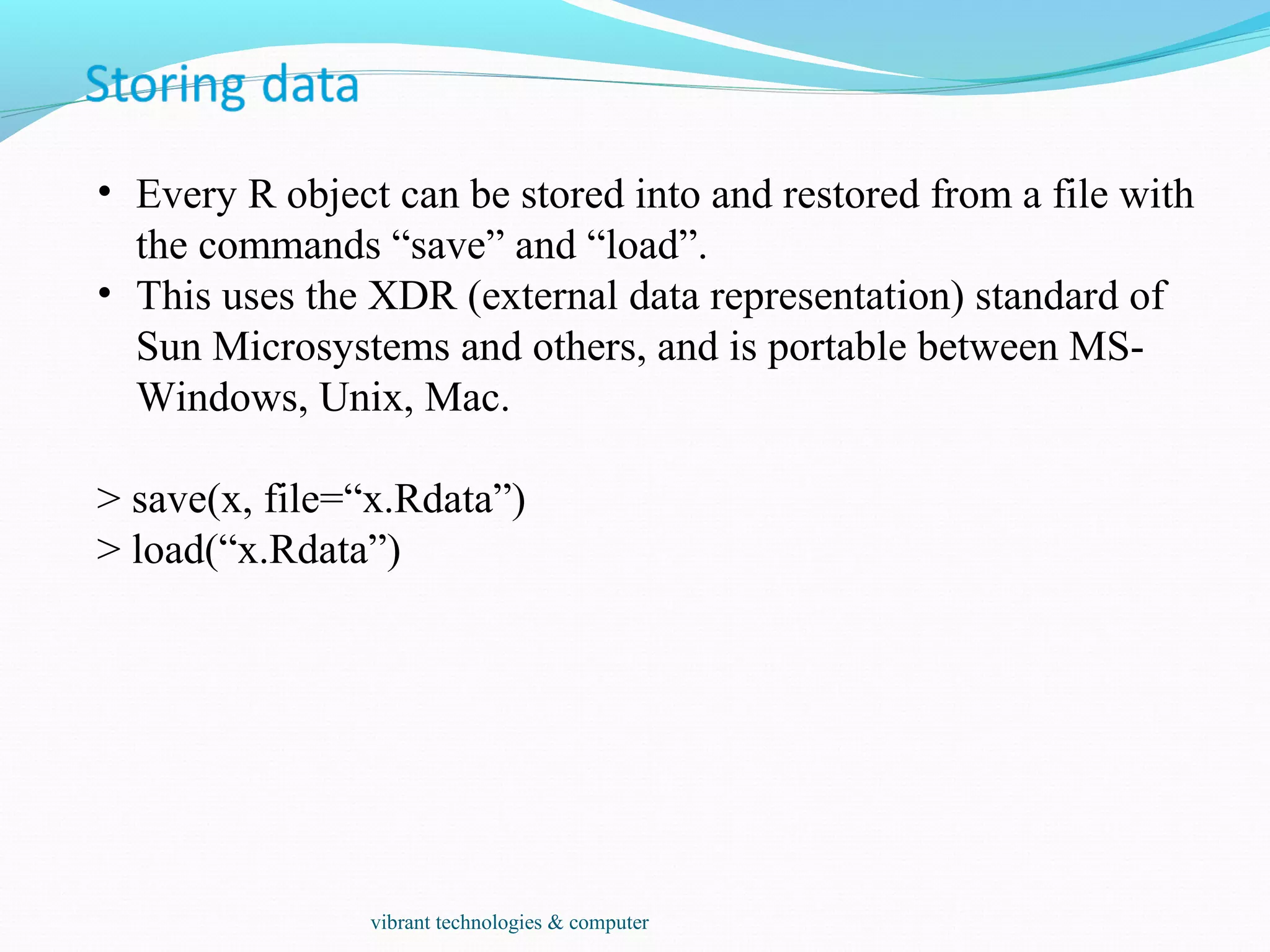
• Every R object can be stored into and restored from a file with
the commands “save” and “load”.
• This uses the XDR (external data representation) standard of
Sun Microsystems and others, and is portable between MS-
Windows, Unix, Mac.
> save(x, file=“x.Rdata”)
> load(“x.Rdata”)
vibrant technologies & computer
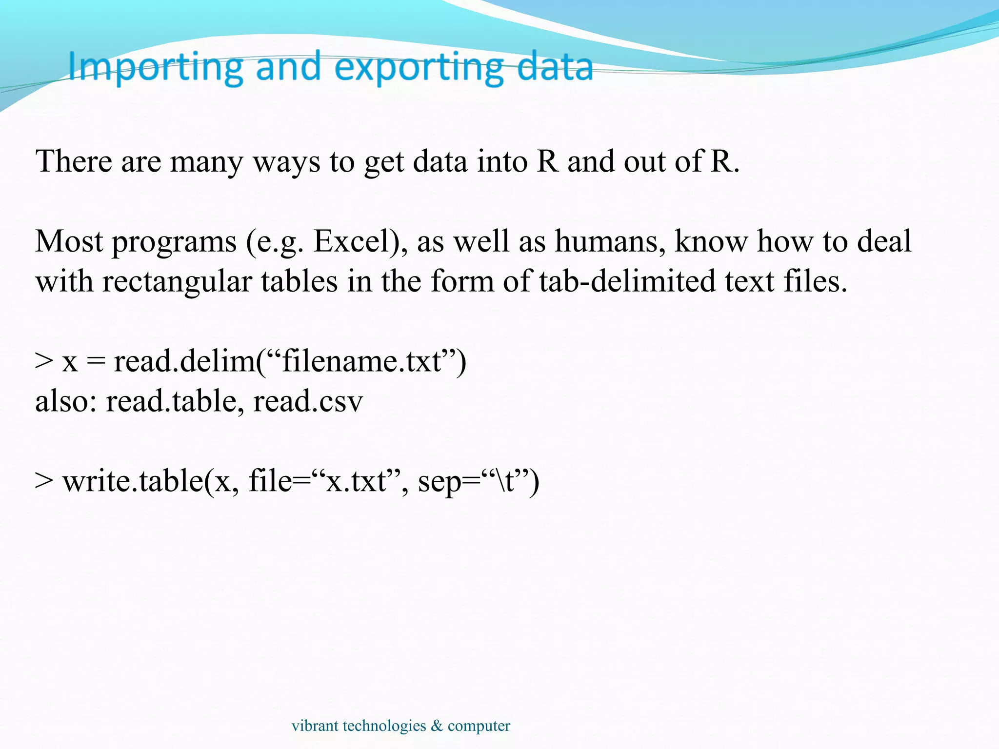
There are many ways to get data into R and out of R.
Most programs (e.g. Excel), as well as humans, know how to deal
with rectangular tables in the form of tab-delimited text files.
> x = read.delim(“filename.txt”)
also: read.table, read.csv
> write.table(x, file=“x.txt”, sep=“t”)
vibrant technologies & computer
Type conversions: by default, the read functions try to guess and
autoconvert the data types of the different columns (e.g. number,
factor, character).
 There are options as.is and colClasses to control this – read
the online help
Special characters: the delimiter character (space, comma,
tabulator) and the end-of-line character cannot be part of a data
field.
 To circumvent this, text may be “quoted”.
 However, if this option is used (the default), then the quote
characters themselves cannot be part of a data field. Except if
they themselves are within quotes…
 Understand the conventions your input files use and set the
quote options accordingly.
vibrant technologies & computer
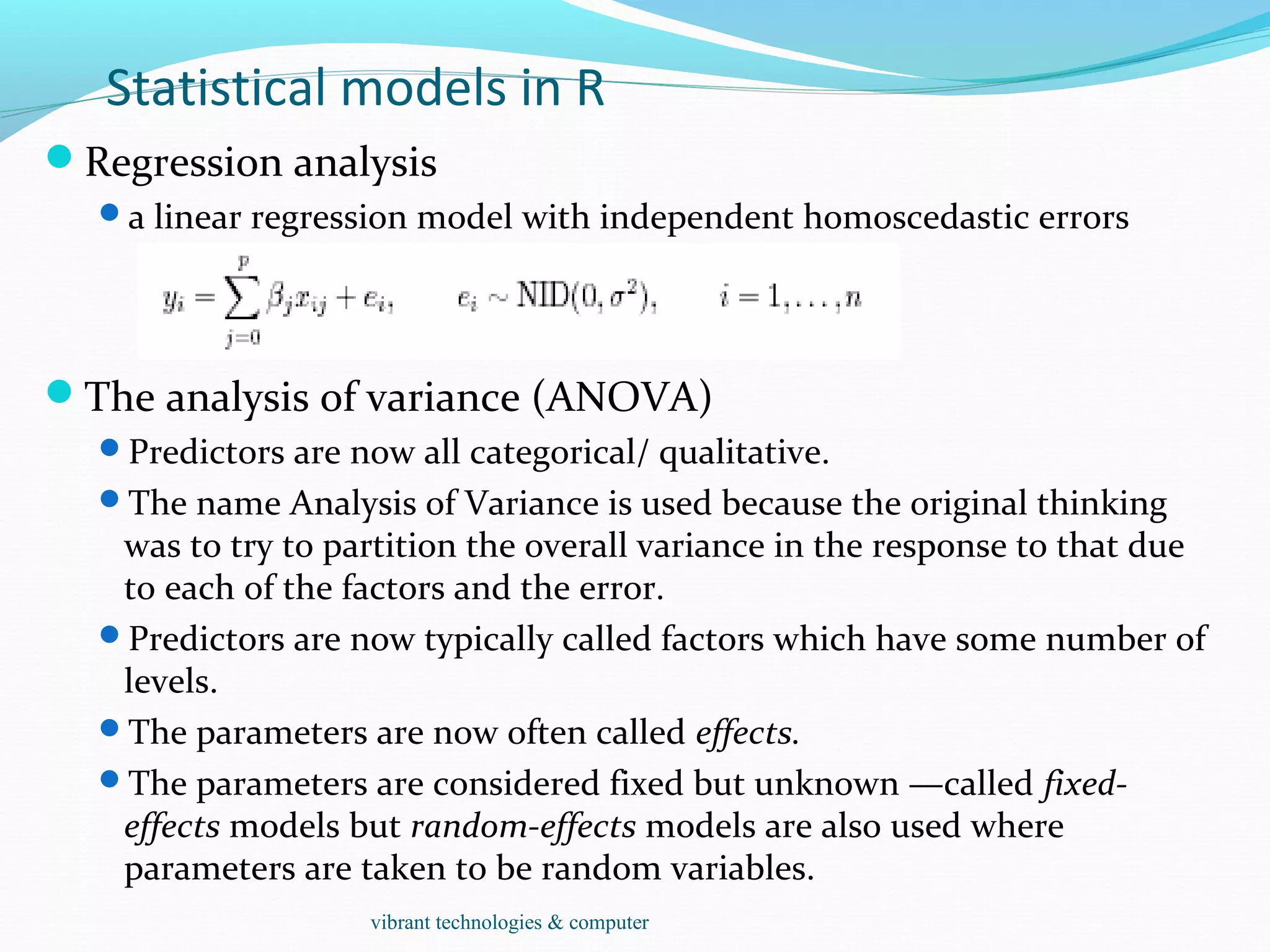
Statistical models in R
Regression analysis
a linear regression model with independent homoscedastic errors
The analysis of variance (ANOVA)
Predictors are now all categorical/ qualitative.
The name Analysis of Variance is used because the original thinking
was to try to partition the overall variance in the response to that due
to each of the factors and the error.
Predictors are now typically called factors which have some number of
levels.
The parameters are now often called effects.
The parameters are considered fixed but unknown —called fixed-
effects models but random-effects models are also used where
parameters are taken to be random variables.
vibrant technologies & computer
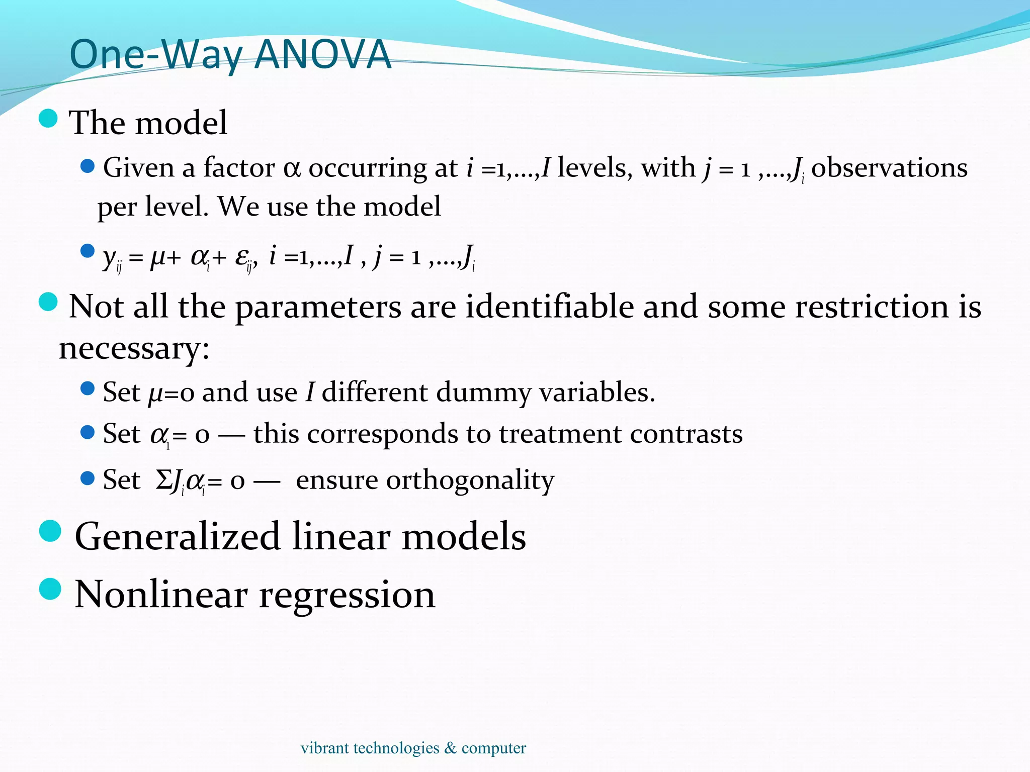
One-Way ANOVA
The model
Given a factor α occurring at i =1,…,I levels, with j = 1 ,…,Ji observations
per level. We use the model
yij = µ+ αi+ εij, i =1,…,I , j = 1 ,…,Ji
Not all the parameters are identifiable and some restriction is
necessary:
Set µ=0 and use I different dummy variables.
Set α1= 0 — this corresponds to treatment contrasts
Set ΣJiαi= 0 — ensure orthogonality
Generalized linear models
Nonlinear regression
vibrant technologies & computer
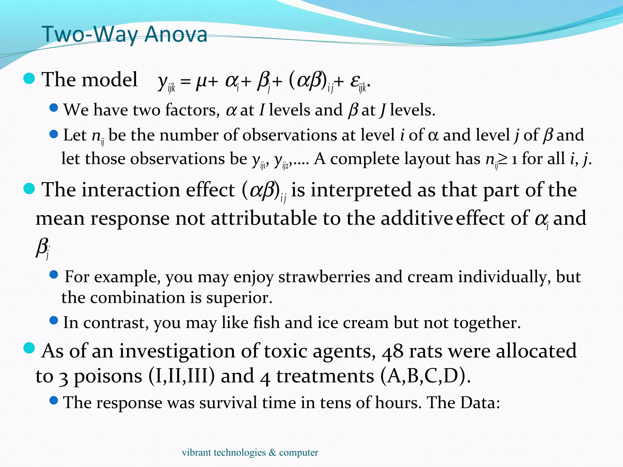
Two-Way Anova
The model yijk = µ+ αi+ βj+ (αβ)ij+ εijk.
We have two factors, α at I levels and β at J levels.
Let nij be the number of observations at level i of α and level j of β and
let those observations be yij1, yij2,…. A complete layout has nij≥ 1 for all i, j.
The interaction effect (αβ)ij is interpreted as that part of the
mean response not attributable to the additiveeffect of αi and
βj
.
For example, you may enjoy strawberries and cream individually, but
the combination is superior.
In contrast, you may like fish and ice cream but not together.
As of an investigation of toxic agents, 48 rats were allocated
to 3 poisons (I,II,III) and 4 treatments (A,B,C,D).
The response was survival time in tens of hours. The Data:
vibrant technologies & computer
Statistical Strategy and Model Uncertainty
Strategy
Diagnostics: Checking of assumptions: constant variance, linearity,
normality, outliers, influential points, serial correlation and collinearity.
Transformation: Transforming the response — Box-Cox, transforming
the predictors — tests and polynomial regression.
Variable selection: Stepwise and criterion based methods
Avoid doing too much analysis.
Remember that fitting the data well is no guarantee of good predictive
performance or that the model is a good representation of the
underlying population.
Avoid complex models for small datasets.
Try to obtain new data to validate your proposed model. Some people
set aside some of their existing data for this purpose.
Use past experience with similar data to guide the choice of model.
vibrant technologies & computer
Simulation and Regression
What is the sampling distribution of least squares estimates
when the noises are not normally distributed?
Assume the noises are independent and identically
distributed.
1. Generate ε from the known error distribution.
2. Form y = Xβ + ε.
3. Compute the estimate of β.
Repeat these three steps many times.
We can estimate the sampling distribution of using the empirical
distribution of the generated , which we can estimate as accurately as
we please by simply running the simulation for long enough.
This technique is useful for a theoretical investigation of the properties
of a proposed new estimator. We can see how its performance
compares to other estimators.
It is of no value for the actual data since we don’t know the true error
distribution and we don’t know β.
vibrant technologies & computer
Bootstrap
The bootstrap method mirrors the simulation method but
uses quantities we do know.
Instead of sampling from the population distribution which we do not
know in practice, we resample from the data itself.
Difficulty: β is unknown and the distribution of ε is known.
Solution: β is replaced by its good estimate b and the
distribution of ε is replaced by the residuals e1,…,en.
1. Generate e* by sampling with replacement from e1,…,en.
2. Form y* = X b + e*.
3. Compute b* from (X, y*).
For small n, it is possible to compute b* for every possible
samples of e1,…,en. 1n
In practice, this number of bootstrap samples can be as small as 50 if
all we want is an estimate of the variance of our estimates but needs to
be larger if confidence intervals are wanted.
vibrant technologies & computer
Implementation
How do we take a sample of residuals with replacement?
sample() is good for generating random samples of indices:
 sample(10,rep=T) leads to “7 9 9 2 5 7 4 1 8 9”
Execute the bootstrap.
Make a matrix to save the results in and then repeat the bootstrap
process 1000 times for a linear regression with five regressors:
bcoef <- matrix(0,1000,6)
Program: for(i in 1:1000){
newy <- g$fit + g$res[sample(47, rep=T)]
brg <- lm(newy~y)
bcoef[i,] <- brg$coef
}
Here g is the output from the data with regression
analysis.
vibrant technologies & computer
Test and Confidence Interval
To test the null hypothesis that H0 : β1 = 0 against the
alternative H1 : β1 > 0, we may figure what fraction of the
bootstrap sampled β1 were less than zero:
length(bcoef[bcoef[,2]<0,2])/1000: It leads to 0.019.
The p-value is 1.9% and we reject the null at the 5% level.
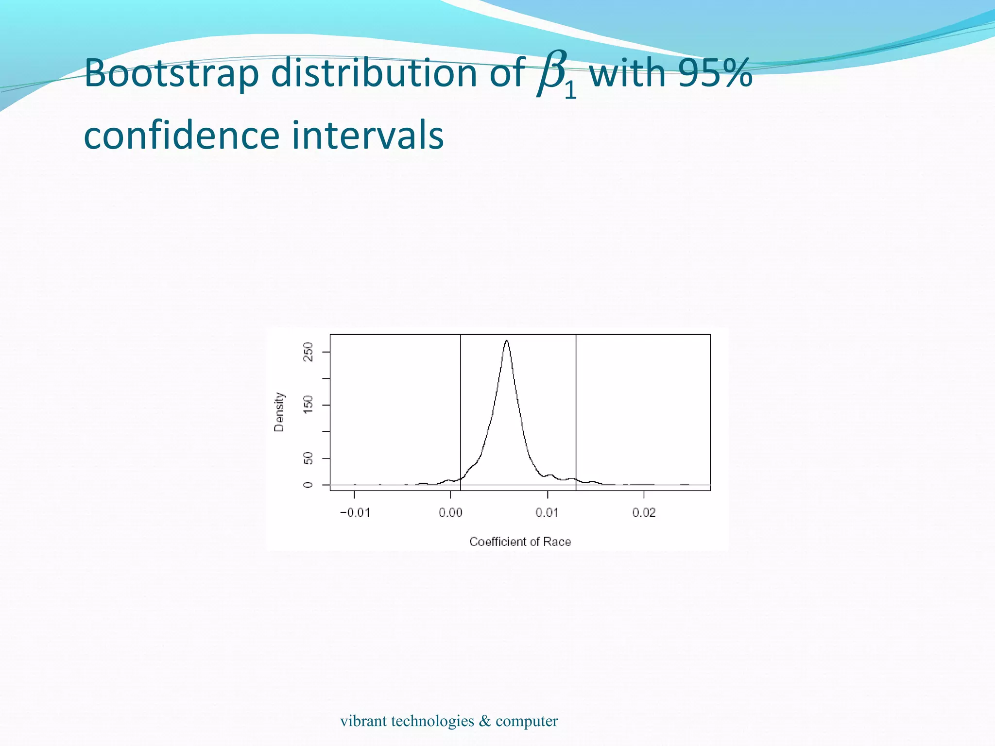
We can also make a 95% confidence interval for this
parameter by taking the empirical quantiles:
quantile(bcoef[,2],c(0.025,0.975))
2.5% 97.5%
0.00099037 0.01292449
We can get a better picture of the distribution by looking at
the density and marking the confidence interval:
plot(density(bcoef[,2]),xlab="Coefficient of Race",main="")
abline(v=quantile(bcoef[,2],c(0.025,0.975)))
vibrant technologies & computer
Bootstrap distribution of β1 with 95%
confidence intervals
vibrant technologies & computer
The Effect of Choice of Kernels
The average amount of annual precipitation (rainfall) in
inches for each of 70 United States (and Puerto Rico) cities.
data(precip)
bw <- bw.SJ(precip) ## sensible automatic choice
plot(density(precip, bw = bw, n = 2^13), main = "same sd
bandwidths, 7 different kernels")
for(i in 2:length(kernels)) lines(density(precip, bw = bw, kern
= kernels[i], n = 2^13), col = i)
vibrant technologies & computer
Explore Association
Data(stackloss)
It is a data frame with 21 observations on 4 variables.
 [,1] `Air Flow' Flow of cooling air
 [,2] `Water Temp' Cooling Water Inlet Temperature
 [,3] `Acid Conc.' Concentration of acid [per 1000, minus
500]
 [,4] `stack.loss' Stack loss
The data sets `stack.x', a matrix with the first three
(independent) variables of the data frame, and `stack.loss',
the numeric vector giving the fourth (dependent) variable,
are provided as well.
Scatterplots, scatterplot matrix:
plot(stackloss$Ai,stackloss$W)
plot(stackloss) data(stackloss)
two quantitative variables.
summary(lm.stack <- lm(stack.loss ~ stack.x))
vibrant technologies & computer
Explore Association
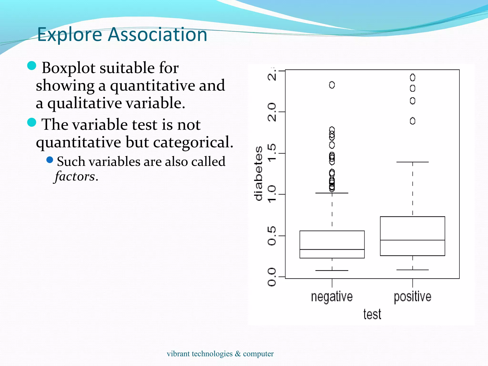
Boxplot suitable for
showing a quantitative and
a qualitative variable.
The variable test is not
quantitative but categorical.
Such variables are also called
factors.
vibrant technologies & computer
LEAST SQUARES ESTIMATION
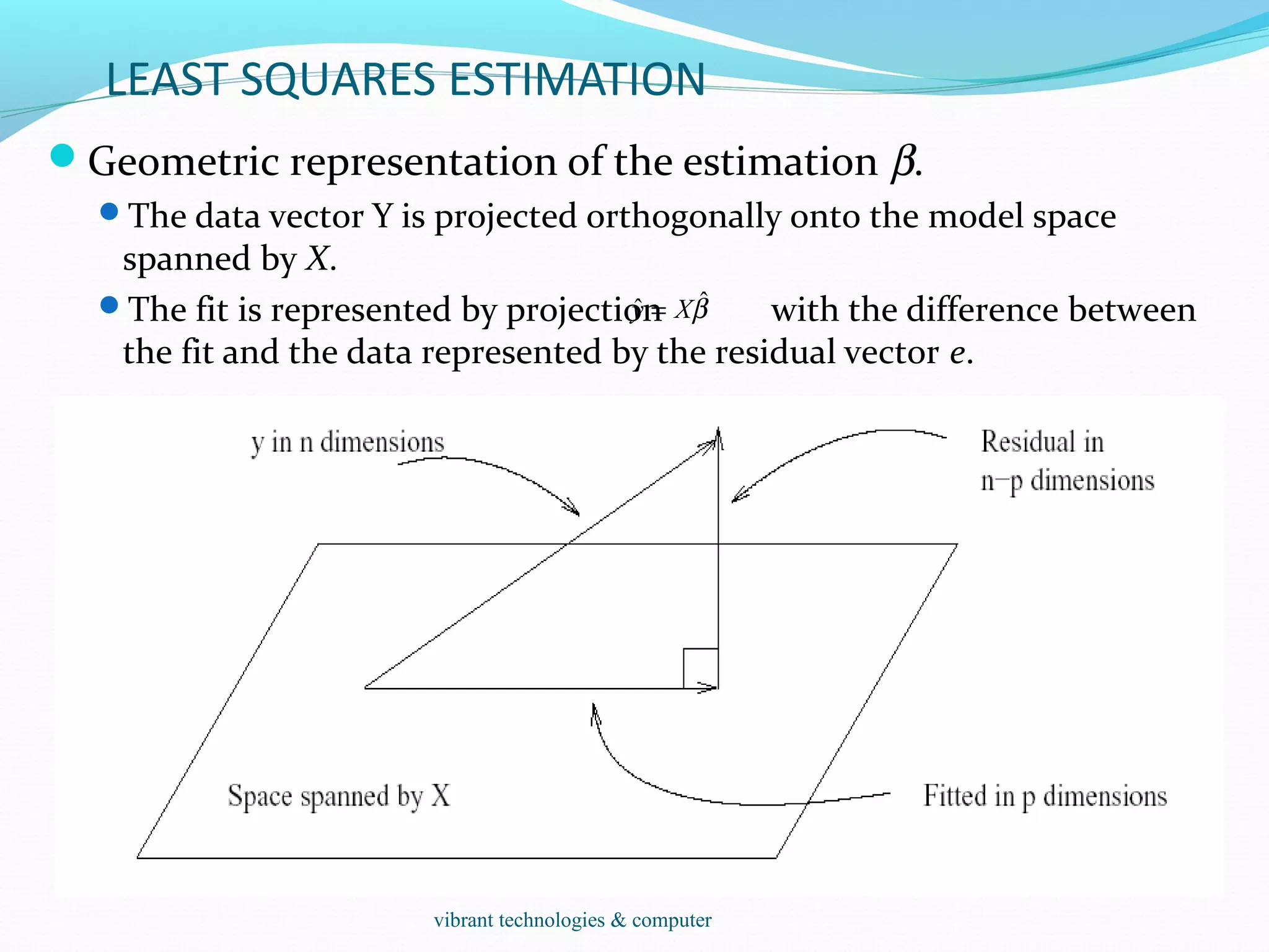
Geometric representation of the estimation β.
The data vector Y is projected orthogonally onto the model space
spanned by X.
The fit is represented by projection with the difference between
the fit and the data represented by the residual vector e.
βˆˆ Xy =
vibrant technologies & computer
Hypothesis tests to compare models
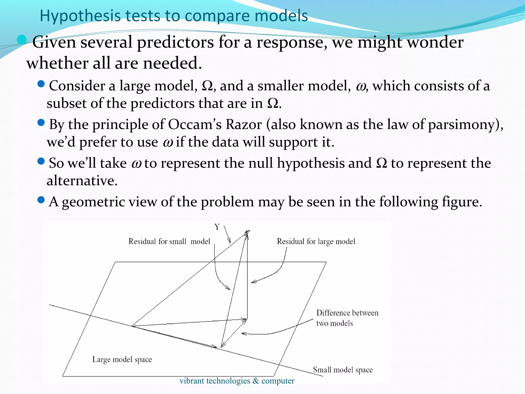
Given several predictors for a response, we might wonder
whether all are needed.
Consider a large model, Ω, and a smaller model, ω, which consists of a
subset of the predictors that are in Ω.
By the principle of Occam’s Razor (also known as the law of parsimony),
we’d prefer to use ω if the data will support it.
So we’ll take ω to represent the null hypothesis and Ω to represent the
alternative.
A geometric view of the problem may be seen in the following figure.
vibrant technologies & computer

R-programming-training-in-mumbai

  • 1.
    Vibrant technologies &computers Vashi Vibranttechnologies.co.in vibrant technologies & computer
  • 2.
  • 3.
    Outline Introduction: Historical development S, Splus Capability StatisticalAnalysis References Calculator Data Type Resources Simulation and Statistical Tables Probability distributions Programming Grouping, loops and conditional execution Function Reading and writing data from files Modeling Regression ANOVA Data Analysis on Association Lottery Geyser Smoothing vibrant technologies & computer
  • 4.
    Introduction R is “GNUS” — A language and environment for data manipula-tion, calculation and graphical display. R is similar to the award-winning S system, which was developed at Bell Laboratories by John Chambers et al. a suite of operators for calculations on arrays, in particular matrices, a large, coherent, integrated collection of intermediate tools for interactive data analysis, graphical facilities for data analysis and display either directly at the computer or on hardcopy a well developed programming language which includes conditionals, loops, user defined recursive functions and input and output facilities. The core of R is an interpreted computer language. It allows branching and looping as well as modular programming using functions. Most of the user-visible functions in R are written in R, calling upon a smaller set of internal primitives. It is possible for the user to interface to procedures written in C, C++ or FORTRAN languages for efficiency, and also to write additionalvibrant technologies & computer
  • 5.
    odata handling andstorage: numeric, textual omatrix algebra ohash tables and regular expressions ohigh-level data analytic and statistical functions oclasses (“OO”) ographics oprogramming language: loops, branching, subroutines ois not a database, but connects to DBMSs ohas no graphical user interfaces, but connects to Java, TclTk olanguage interpreter can be very slow, but allows to call own C/C++ code ono spreadsheet view of data, but connects to Excel/MsOffice ono professional / commercial support vibrant technologies & computer
  • 6.
    o Packaging: acrucial infrastructure to efficiently produce, load and keep consistent software libraries from (many) different sources / authors o Statistics: most packages deal with statistics and data analysis o State of the art: many statistical researchers provide their methods as R packages vibrant technologies & computer
  • 7.
    Data Analysis andPresentation The R distribution contains functionality for large number of statistical procedures. linear and generalized linear models nonlinear regression models time series analysis classical parametric and nonparametric tests clustering smoothing R also has a large set of functions which provide a flexible graphical environment for creating various kinds of data presentations. vibrant technologies & computer
  • 8.
    References For R, The basicreference is The New S Language: A Programming Environment for Data Analysis and Graphics by Richard A. Becker, John M. Chambers and Allan R. Wilks (the “Blue Book”) . The new features of the 1991 release of S (S version 3) are covered in Statistical Models in S edited by John M. Chambers and Trevor J. Hastie (the “White Book”). Classical and modern statistical techniques have been implemented.  Some of these are built into the base R environment.  Many are supplied as packages. There are about 8 packages supplied with R (called “standard” packages) and many more are available through the cran family of Internet sites (via http://cran.r-project.org). All the R functions have been documented in the form of help pages in an “output independent” form which can be used to create versions for HTML, LATEX, text etc. The document “An Introduction to R” provides a more user-friendly starting point. An “R Language Definition” manual More specialized manuals on data import/export and extending R. vibrant technologies & computer
  • 9.
    > log2(32) [1] 5 >sqrt(2) [1] 1.414214 > seq(0, 5, length=6) [1] 0 1 2 3 4 5 > plot(sin(seq(0, 2*pi, length=100))) 0 20 40 60 80 100 -1.0-0.50.00.51.0 Index sin(seq(0,2*pi,length=100)) vibrant technologies & computer
  • 10.
    primitive (or: atomic)data types in R are: • numeric (integer, double, complex) • character • logical • function out of these, vectors, arrays, lists can be built. vibrant technologies & computer
  • 11.
    • Object: acollection of atomic variables and/or other objects that belong together • Example: a microarray experiment • probe intensities • patient data (tissue location, diagnosis, follow-up) • gene data (sequence, IDs, annotation) Parlance: • class: the “abstract” definition of it • object: a concrete instance • method: other word for ‘function’ • slot: a component of an object vibrant technologies & computer
  • 12.
    Advantages: Encapsulation (can usethe objects and methods someone else has written without having to care about the internals) Generic functions (e.g. plot, print) Inheritance (hierarchical organization of complexity) Caveat: Overcomplicated, baroque program architecture… vibrant technologies & computer
  • 13.
    > a =49 > sqrt(a) [1] 7 > a = "The dog ate my homework" > sub("dog","cat",a) [1] "The cat ate my homework“ > a = (1+1==3) > a [1] FALSE numeric character string logical vibrant technologies & computer
  • 14.
    • vector: anordered collection of data of the same type > a = c(1,2,3) > a*2 [1] 2 4 6 • Example: the mean spot intensities of all 15488 spots on a chip: a vector of 15488 numbers • In R, a single number is the special case of a vector with 1 element. • Other vector types: character strings, logical vibrant technologies & computer
  • 15.
    • matrix: arectangular table of data of the same type • example: the expression values for 10000 genes for 30 tissue biopsies: a matrix with 10000 rows and 30 columns. • array: 3-,4-,..dimensional matrix • example: the red and green foreground and background values for 20000 spots on 120 chips: a 4 x 20000 x 120 (3D) array. vibrant technologies & computer
  • 16.
    • vector: anordered collection of data of the same type. > a = c(7,5,1) > a[2] [1] 5 • list: an ordered collection of data of arbitrary types. > doe = list(name="john",age=28,married=F) > doe$name [1] "john“ > doe$age [1] 28 • Typically, vector elements are accessed by their index (an integer), list elements by their name (a character string). But both types support both access methods. vibrant technologies & computer
  • 17.
    data frame: issupposed to represent the typical data table that researchers come up with – like a spreadsheet. It is a rectangular table with rows and columns; data within each column has the same type (e.g. number, text, logical), but different columns may have different types. Example: > a localisation tumorsize progress XX348 proximal 6.3 FALSE XX234 distal 8.0 TRUE XX987 proximal 10.0 FALSE vibrant technologies & computer
  • 18.
    A character stringcan contain arbitrary text. Sometimes it is useful to use a limited vocabulary, with a small number of allowed words. A factor is a variable that can only take such a limited number of values, which are called levels. > a [1] Kolon(Rektum) Magen Magen [4] Magen Magen Retroperitoneal [7] Magen Magen(retrogastral) Magen Levels: Kolon(Rektum) Magen Magen(retrogastral) Retroperitoneal > class(a) [1] "factor" > as.character(a) [1] "Kolon(Rektum)" "Magen" "Magen" [4] "Magen" "Magen" "Retroperitoneal" [7] "Magen" "Magen(retrogastral)" "Magen" > as.integer(a) [1] 1 2 2 2 2 4 2 3 2 > as.integer(as.character(a)) [1] NA NA NA NA NA NA NA NA NA NA NA NA Warning message: NAs introduced by coercion vibrant technologies & computer
  • 19.
    Individual elements ofa vector, matrix, array or data frame are accessed with “[ ]” by specifying their index, or their name > a localisation tumorsize progress XX348 proximal 6.3 0 XX234 distal 8.0 1 XX987 proximal 10.0 0 > a[3, 2] [1] 10 > a["XX987", "tumorsize"] [1] 10 > a["XX987",] localisation tumorsize progress XX987 proximal 10 0 vibrant technologies & computer
  • 20.
    > a localisation tumorsizeprogress XX348 proximal 6.3 0 XX234 distal 8.0 1 XX987 proximal 10.0 0 > a[c(1,3),] localisation tumorsize progress XX348 proximal 6.3 0 XX987 proximal 10.0 0 > a[c(T,F,T),] localisation tumorsize progress XX348 proximal 6.3 0 XX987 proximal 10.0 0 > a$localisation [1] "proximal" "distal" "proximal" > a$localisation=="proximal" [1] TRUE FALSE TRUE > a[ a$localisation=="proximal", ] localisation tumorsize progress XX348 proximal 6.3 0 XX987 proximal 10.0 0 subset rows by a vector of indices subset rows by a logical vector subset a column comparison resulting in logical vector subset the selected rows vibrant technologies & computer
  • 21.
    Resources A package specificationallows the production of loadable modules for specific purposes, and several contributed packages are made available through the CRAN sites. CRAN and R homepage: http://www.r-project.org/ It is R’s central homepage, giving information on the R project and everything related to it. http://cran.r-project.org/ It acts as the download area,carrying the software itself, extension packages, PDF manuals. Getting help with functions and features help(solve) ?solve For a feature specified by special characters, the argument must be enclosed in double or single quotes, making it a “character string”: help("[[") vibrant technologies & computer
  • 22.
    Details about aspecific command whose name you know (input arguments, options, algorithm, results): >? t.test or >help(t.test) vibrant technologies & computer
  • 23.
  • 24.
    Probability distributions Cumulative distributionfunction P(X ≤ x): ‘p’ for the CDF Probability density function: ‘d’ for the density,, Quantile function (given q, the smallest x such that P(X ≤ x) > q): ‘q’ for the quantile simulate from the distribution: ‘r Distribution R name additional arguments beta beta shape1, shape2, ncp binomial binom size, prob Cauchy cauchy location, scale chi-squared chisq df, ncp exponential exp rate F f df1, df1, ncp gamma gamma shape, scale geometric geom prob hypergeometric hyper m, n, k log-normal lnorm meanlog, sdlog logistic logis; negative binomial nbinom; normal norm; Poisson pois; Student’s t t ; uniform unif; Weibull weibull; Wilcoxon wilcox vibrant technologies & computer
  • 25.
    Grouping, loops andconditional execution Grouped expressions R is an expression language in the sense that its only command type is a function or expression which returns a result. Commands may be grouped together in braces, {expr 1, . . ., expr m}, in which case the value of the group is the result of the last expression in the group evaluated. Control statements if statements The language has available a conditional construction of the form if (expr 1) expr 2 else expr 3 where expr 1 must evaluate to a logical value and the result of the entire expression is then evident. a vectorized version of the if/else construct, the ifelse function. This has the form ifelse(condition, a, b) vibrant technologies & computer
  • 26.
    Repetitive execution for loops,repeat and while for (name in expr 1) expr 2 where name is the loop variable. expr 1 is a vector expression, (often a sequence like 1:20), and expr 2 is often a grouped expression with its sub-expressions written in terms of the dummy name. expr 2 is repeatedly evaluated as name ranges through the values in the vector result of expr 1. Other looping facilities include the repeat expr statement and the while (condition) expr statement. The break statement can be used to terminate any loop, possibly abnormally. This is the only way to terminate repeat loops. The next statement can be used to discontinue one particular cycle and skip to the “next”. vibrant technologies & computer
  • 27.
    if (logical expression){ statements } else { alternative statements } else branch is optional vibrant technologies & computer
  • 28.
    • When thesame or similar tasks need to be performed multiple times; for all elements of a list; for all columns of an array; etc. • Monte Carlo Simulation • Cross-Validation (delete one and etc) for(i in 1:10) { print(i*i) } i=1 while(i<=10) { print(i*i) i=i+sqrt(i) } vibrant technologies & computer
  • 29.
    • When thesame or similar tasks need to be performed multiple times for all elements of a list or for all columns of an array. • May be easier and faster than “for” loops • lapply(li, function ) • To each element of the list li, the function function is applied. • The result is a list whose elements are the individual function results. > li = list("klaus","martin","georg") > lapply(li, toupper) > [[1]] > [1] "KLAUS" > [[2]] > [1] "MARTIN" > [[3]] > [1] "GEORG" vibrant technologies & computer
  • 30.
    sapply( li, fct) Like apply, but tries to simplify the result, by converting it into a vector or array of appropriate size > li = list("klaus","martin","georg") > sapply(li, toupper) [1] "KLAUS" "MARTIN" "GEORG" > fct = function(x) { return(c(x, x*x, x*x*x)) } > sapply(1:5, fct) [,1] [,2] [,3] [,4] [,5] [1,] 1 2 3 4 5 [2,] 1 4 9 16 25 [3,] 1 8 27 64 125 vibrant technologies & computer
  • 31.
    apply( arr, margin,fct ) Apply the function fct along some dimensions of the array arr, according to margin, and return a vector or array of the appropriate size. > x [,1] [,2] [,3] [1,] 5 7 0 [2,] 7 9 8 [3,] 4 6 7 [4,] 6 3 5 > apply(x, 1, sum) [1] 12 24 17 14 > apply(x, 2, sum) [1] 22 25 20 vibrant technologies & computer
  • 32.
    Functions do thingswith data “Input”: function arguments (0,1,2,…) “Output”: function result (exactly one) Example: add = function(a,b) { result = a+b return(result) } Operators: Short-cut writing for frequently used functions of one or two arguments. Examples: + - * / ! & | %% vibrant technologies & computer
  • 33.
    • Functions dothings with data • “Input”: function arguments (0,1,2,…) • “Output”: function result (exactly one) Exceptions to the rule: • Functions may also use data that sits around in other places, not just in their argument list: “scoping rules”* • Functions may also do other things than returning a result. E.g., plot something on the screen: “side effects” * Lexical scope and Statistical Computing. R. Gentleman, R. Ihaka, Journal of Computational and Graphical Statistics, 9(3), p. 491-508 (2000). vibrant technologies & computer
  • 34.
    Reading data fromfiles The read.table() function To read an entire data frame directly, the external file will normally have a special form. The first line of the file should have a name for each variable in the data frame. Each additional line of the file has its first item a row label and the values for each variable. Price Floor Area Rooms Age Cent.heat 01 52.00 111.0 830 5 6.2 no 02 54.75 128.0 710 5 7.5 no 03 57.50 101.0 1000 5 4.2 no 04 57.50 131.0 690 6 8.8 no 05 59.75 93.0 900 5 1.9 yes ... numeric variables and nonnumeric variables (factors) vibrant technologies & computer
  • 35.
    Reading data fromfiles HousePrice <- read.table("houses.data", header=TRUE) Price Floor Area Rooms Age Cent.heat 52.00 111.0 830 5 6.2 no 54.75 128.0 710 5 7.5 no 57.50 101.0 1000 5 4.2 no 57.50 131.0 690 6 8.8 no 59.75 93.0 900 5 1.9 yes ... The data file is named ‘input.dat’. Suppose the data vectors are of equal length and are to be read in in parallel. Suppose that there are three vectors, the first of mode character and the remaining two of mode numeric. The scan() function inp<- scan("input.dat", list("",0,0)) To separate the data items into three separate vectors, use assignments like label <- inp[[1]]; x <- inp[[2]]; y <- inp[[3]] inp <- scan("input.dat", list(id="", x=0, y=0)); inp$id; inp$x; inp$y vibrant technologies & computer
  • 36.
    • Every Robject can be stored into and restored from a file with the commands “save” and “load”. • This uses the XDR (external data representation) standard of Sun Microsystems and others, and is portable between MS- Windows, Unix, Mac. > save(x, file=“x.Rdata”) > load(“x.Rdata”) vibrant technologies & computer
  • 37.
    There are manyways to get data into R and out of R. Most programs (e.g. Excel), as well as humans, know how to deal with rectangular tables in the form of tab-delimited text files. > x = read.delim(“filename.txt”) also: read.table, read.csv > write.table(x, file=“x.txt”, sep=“t”) vibrant technologies & computer
  • 38.
    Type conversions: bydefault, the read functions try to guess and autoconvert the data types of the different columns (e.g. number, factor, character).  There are options as.is and colClasses to control this – read the online help Special characters: the delimiter character (space, comma, tabulator) and the end-of-line character cannot be part of a data field.  To circumvent this, text may be “quoted”.  However, if this option is used (the default), then the quote characters themselves cannot be part of a data field. Except if they themselves are within quotes…  Understand the conventions your input files use and set the quote options accordingly. vibrant technologies & computer
  • 39.
    Statistical models inR Regression analysis a linear regression model with independent homoscedastic errors The analysis of variance (ANOVA) Predictors are now all categorical/ qualitative. The name Analysis of Variance is used because the original thinking was to try to partition the overall variance in the response to that due to each of the factors and the error. Predictors are now typically called factors which have some number of levels. The parameters are now often called effects. The parameters are considered fixed but unknown —called fixed- effects models but random-effects models are also used where parameters are taken to be random variables. vibrant technologies & computer
  • 40.
    One-Way ANOVA The model Givena factor α occurring at i =1,…,I levels, with j = 1 ,…,Ji observations per level. We use the model yij = µ+ αi+ εij, i =1,…,I , j = 1 ,…,Ji Not all the parameters are identifiable and some restriction is necessary: Set µ=0 and use I different dummy variables. Set α1= 0 — this corresponds to treatment contrasts Set ΣJiαi= 0 — ensure orthogonality Generalized linear models Nonlinear regression vibrant technologies & computer
  • 41.
    Two-Way Anova The modelyijk = µ+ αi+ βj+ (αβ)ij+ εijk. We have two factors, α at I levels and β at J levels. Let nij be the number of observations at level i of α and level j of β and let those observations be yij1, yij2,…. A complete layout has nij≥ 1 for all i, j. The interaction effect (αβ)ij is interpreted as that part of the mean response not attributable to the additiveeffect of αi and βj . For example, you may enjoy strawberries and cream individually, but the combination is superior. In contrast, you may like fish and ice cream but not together. As of an investigation of toxic agents, 48 rats were allocated to 3 poisons (I,II,III) and 4 treatments (A,B,C,D). The response was survival time in tens of hours. The Data: vibrant technologies & computer
  • 42.
    Statistical Strategy andModel Uncertainty Strategy Diagnostics: Checking of assumptions: constant variance, linearity, normality, outliers, influential points, serial correlation and collinearity. Transformation: Transforming the response — Box-Cox, transforming the predictors — tests and polynomial regression. Variable selection: Stepwise and criterion based methods Avoid doing too much analysis. Remember that fitting the data well is no guarantee of good predictive performance or that the model is a good representation of the underlying population. Avoid complex models for small datasets. Try to obtain new data to validate your proposed model. Some people set aside some of their existing data for this purpose. Use past experience with similar data to guide the choice of model. vibrant technologies & computer
  • 43.
    Simulation and Regression Whatis the sampling distribution of least squares estimates when the noises are not normally distributed? Assume the noises are independent and identically distributed. 1. Generate ε from the known error distribution. 2. Form y = Xβ + ε. 3. Compute the estimate of β. Repeat these three steps many times. We can estimate the sampling distribution of using the empirical distribution of the generated , which we can estimate as accurately as we please by simply running the simulation for long enough. This technique is useful for a theoretical investigation of the properties of a proposed new estimator. We can see how its performance compares to other estimators. It is of no value for the actual data since we don’t know the true error distribution and we don’t know β. vibrant technologies & computer
  • 44.
    Bootstrap The bootstrap methodmirrors the simulation method but uses quantities we do know. Instead of sampling from the population distribution which we do not know in practice, we resample from the data itself. Difficulty: β is unknown and the distribution of ε is known. Solution: β is replaced by its good estimate b and the distribution of ε is replaced by the residuals e1,…,en. 1. Generate e* by sampling with replacement from e1,…,en. 2. Form y* = X b + e*. 3. Compute b* from (X, y*). For small n, it is possible to compute b* for every possible samples of e1,…,en. 1n In practice, this number of bootstrap samples can be as small as 50 if all we want is an estimate of the variance of our estimates but needs to be larger if confidence intervals are wanted. vibrant technologies & computer
  • 45.
    Implementation How do wetake a sample of residuals with replacement? sample() is good for generating random samples of indices:  sample(10,rep=T) leads to “7 9 9 2 5 7 4 1 8 9” Execute the bootstrap. Make a matrix to save the results in and then repeat the bootstrap process 1000 times for a linear regression with five regressors: bcoef <- matrix(0,1000,6) Program: for(i in 1:1000){ newy <- g$fit + g$res[sample(47, rep=T)] brg <- lm(newy~y) bcoef[i,] <- brg$coef } Here g is the output from the data with regression analysis. vibrant technologies & computer
  • 46.
    Test and ConfidenceInterval To test the null hypothesis that H0 : β1 = 0 against the alternative H1 : β1 > 0, we may figure what fraction of the bootstrap sampled β1 were less than zero: length(bcoef[bcoef[,2]<0,2])/1000: It leads to 0.019. The p-value is 1.9% and we reject the null at the 5% level. We can also make a 95% confidence interval for this parameter by taking the empirical quantiles: quantile(bcoef[,2],c(0.025,0.975)) 2.5% 97.5% 0.00099037 0.01292449 We can get a better picture of the distribution by looking at the density and marking the confidence interval: plot(density(bcoef[,2]),xlab="Coefficient of Race",main="") abline(v=quantile(bcoef[,2],c(0.025,0.975))) vibrant technologies & computer
  • 47.
    Bootstrap distribution ofβ1 with 95% confidence intervals vibrant technologies & computer
  • 48.
    The Effect ofChoice of Kernels The average amount of annual precipitation (rainfall) in inches for each of 70 United States (and Puerto Rico) cities. data(precip) bw <- bw.SJ(precip) ## sensible automatic choice plot(density(precip, bw = bw, n = 2^13), main = "same sd bandwidths, 7 different kernels") for(i in 2:length(kernels)) lines(density(precip, bw = bw, kern = kernels[i], n = 2^13), col = i) vibrant technologies & computer
  • 49.
    Explore Association Data(stackloss) It isa data frame with 21 observations on 4 variables.  [,1] `Air Flow' Flow of cooling air  [,2] `Water Temp' Cooling Water Inlet Temperature  [,3] `Acid Conc.' Concentration of acid [per 1000, minus 500]  [,4] `stack.loss' Stack loss The data sets `stack.x', a matrix with the first three (independent) variables of the data frame, and `stack.loss', the numeric vector giving the fourth (dependent) variable, are provided as well. Scatterplots, scatterplot matrix: plot(stackloss$Ai,stackloss$W) plot(stackloss) data(stackloss) two quantitative variables. summary(lm.stack <- lm(stack.loss ~ stack.x)) summary(lm.stack <- lm(stack.loss ~ stack.x)) vibrant technologies & computer
  • 50.
    Explore Association Boxplot suitablefor showing a quantitative and a qualitative variable. The variable test is not quantitative but categorical. Such variables are also called factors. vibrant technologies & computer
  • 51.
    LEAST SQUARES ESTIMATION Geometricrepresentation of the estimation β. The data vector Y is projected orthogonally onto the model space spanned by X. The fit is represented by projection with the difference between the fit and the data represented by the residual vector e. βˆˆ Xy = vibrant technologies & computer
  • 52.
    Hypothesis tests tocompare models Given several predictors for a response, we might wonder whether all are needed. Consider a large model, Ω, and a smaller model, ω, which consists of a subset of the predictors that are in Ω. By the principle of Occam’s Razor (also known as the law of parsimony), we’d prefer to use ω if the data will support it. So we’ll take ω to represent the null hypothesis and Ω to represent the alternative. A geometric view of the problem may be seen in the following figure. vibrant technologies & computer
  • 53.
  • 54.