Downloaded 24 times
![14
1890
Frederick Taylor
Scientific
Management
[Industrial
Engineering]
1900
•Henry Gannt
[Project Scheduling]
•Andrey A. Markov
[Markov Processes]
•Assignment
[Networks]
1910
•F. W. Harris
[Inventory Theory]
•E. K. Erlang
[Queuing Theory]
1920
•William Shewart
[Control Charts]
•H.Dodge – H.Roming
[Quality Theory]
1930
Jon Von Neuman –
Oscar Morgenstern
[Game Theory]
1940
•World War 2
•George Dantzig
[Linear
Programming]
•First Computer
1950
•H.Kuhn - A.Tucker
[Non-Linear Prog.]
•Ralph Gomory
[Integer Prog.]
•PERT/CPM
•Richard Bellman
[Dynamic Prog.]
ORSA and TIMS
1960
•John D.C. Litle
[Queuing Theory]
•Simscript - GPSS
[Simulation]
1970
•Microcomputer
1980
•H. Karmarkar
[Linear Prog.]
•Personal computer
•OR/MS Softwares
1990
•Spreadsheet
Packages
•INFORMS
2000……
History of oR](https://image.slidesharecdn.com/resourcemanagementtechniques-190123131615/85/Resource-management-techniques-14-320.jpg)
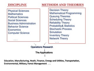
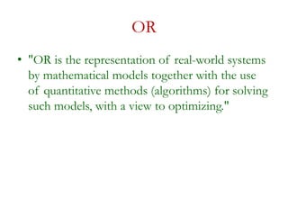
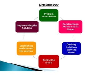
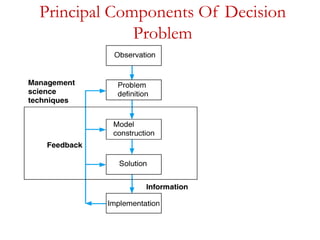


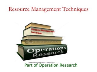
Resource management techniques involve efficiently using an organization's limited resources such as employees, equipment, and finances. Some key techniques include: 1. Linear programming, which uses mathematical models to determine the optimal allocation of resources to meet objectives and constraints. An example is determining the optimal product mix. 2. Operations research, which applies scientific principles and quantitative analysis to help maximize efficiency. It has been widely used by militaries and businesses since World War II. 3. Modeling real-world problems mathematically and using algorithms to determine the best solutions while optimizing objectives under constraints. This allows organizations to best utilize their resources.