This document summarizes a master's thesis that investigated the impact of horizontal projections like balconies on external fire spread on building facades through numerical modeling. It conducted a literature review and validated a fire dynamics simulation program (FDS) against experimental data. Comparative analyses using FDS then compared scenarios with different balcony depths or spandrel heights. The analyses found that balconies at least 60 cm deep resulted in lower risks of external fire spread above the balcony compared to scenarios with only spandrel heights, representing a reduction in risk level allowed by building codes. Balconies of 60-100 cm also reduced surface temperatures above openings by 15-50%. Therefore, a balcony at least 60 cm deep can replace a 1


![6
explained in Chapter 6.6. From this, two types of graphs were produced describing 𝑇𝐴𝑆𝑇 and 𝑞̇ 𝐼𝑁𝐶
′′
as a
function of the height above the opening. These results served as a basis for the determination of
consequences of the given scenario.
The above also means that the results from the Spandrel-case take into account the protection method stated
by the general recommendations in the prescriptive design of the BBR, as discussed in the background in
Chapter 1.1, since a spandrel height of 1.2 m is covered.
The use of 𝑇𝐴𝑆𝑇 and 𝑞̇ 𝐼𝑁𝐶
′′
as proxy variables for the consequence is justified because these variables take into
account the gas temperatures as well as the incident radiation perspective from the fire. These proxy variables
are independent of the type of building material used in the simulations and from the validation study these
variables were also shown to give promising results for this particular problem area.
The relative comparison of consequences was achieved by comparing scenarios from each of the two cases in
the same diagram. More specifically the scenarios that were compared were the combinations given by the
numbers in each of the scenarios in Figure 2.2-2.3. In other words, for these combinations of scenarios the
additions of balconies of various sizes were the only difference in input.
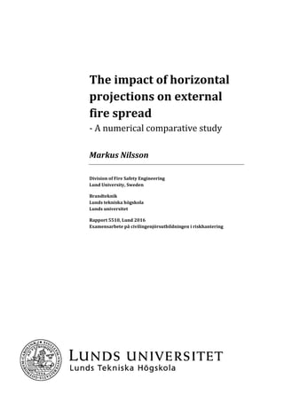
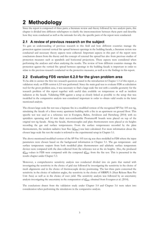
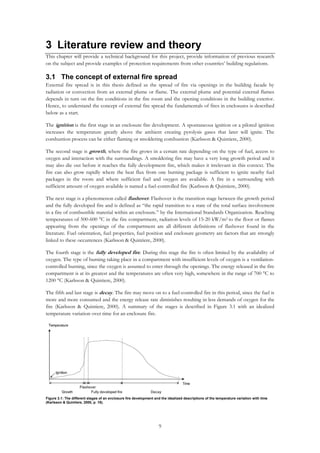
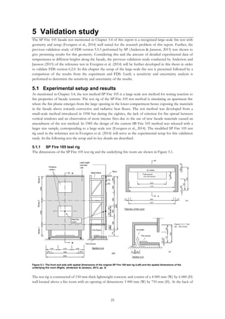
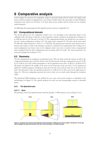
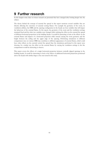
To explain how the results were analysed an example is shown below. In Figure 2.4 an example of 𝑇𝐴𝑆𝑇 as a
function of the height above the opening is shown for four different scenarios.
Since the criteria found in the general advices when performing alternative solution in Sweden are mainly
based on evacuation safety (Boverket, 2013), it is difficult in this case to define a risk criterion from which the
calculated consequences will be compared against. Instead, the consequences given the Spandrel-case were
considered to represent the risk level for the given geometry, design fire, ventilation properties and opening
configuration. The results in Figure 2.4 will answer the following research question stated in Chapter 1.3:
What impact does a horizontal projection have on the fire in regards to temperature and receiving
radiation at the overlying facade?
In Figure 2.4 it is seen that the use of Balcony 2 and 3 results in values that are consistently lower than the
Spandrel-case, hence the existence of these balconies results in lower 𝑇𝐴𝑆𝑇 at the facade on all heights compared
with the Spandrel-case. The use of Balcony 1 however results in higher values from 1 m to 3.2 m above the
opening. These conclusions will also answer the first part of the second research question:
How is the risk level for the risk of fire spread through openings along the building exterior affected
by different protection measures? And how are these risk levels compared with the risk level
accepted in the Swedish building regulations?
50
100
150
200
250
300
350
400
0.6 0.8 1 1.2 1.4 1.6 1.8 2 2.2 2.4 2.6 2.8 3 3.2
Adiabaticsurfacetemperature[ºC]
Height above door [m]
Figure 2.4: Example of adiabatic surface temperature as a
function of the height above the opening in the building facade for
various scenarios.
Figure 2.5: Example of normalized adiabatic surface temperature
values to the Spandrel-case 1.2 m above the opening. The point
of origin for the normalization is seen as a cross on the
Spandrel-case line.
0.3
0.4
0.5
0.6
0.7
0.8
0.9
1
1.1
1.2
1.3
1.4
1.5
1.6
0.6 0.8 1 1.2 1.4 1.6 1.8 2 2.2 2.4 2.6 2.8 3 3.2
Relativeexposure[-]
Height above door [m]
BBR Limit](https://image.slidesharecdn.com/b9c25bc4-7009-433b-9915-9df65ba0719b-160222143636/85/Report_5510_Markus_Nilsson-18-320.jpg)


![23
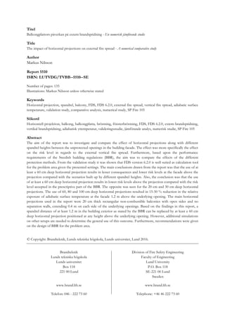
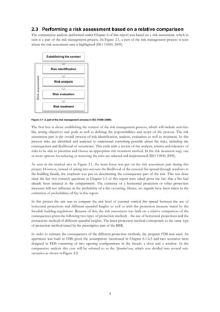
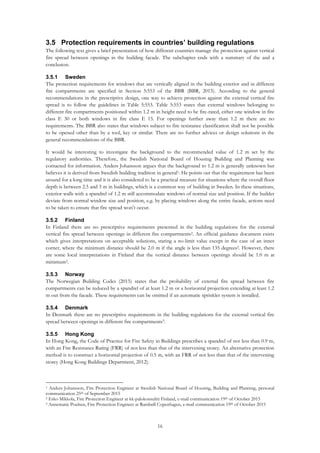
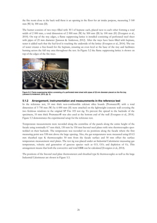
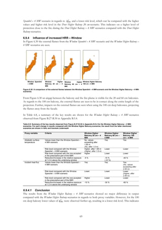
4.5 Adiabatic surface temperature
In FDS there is a way of expressing an artificial effective temperature that is both taking into account the
incident radiation temperature 𝑇𝑟 and the gas temperature 𝑇𝑔: the adiabatic surface temperature 𝑇𝐴𝑆𝑇
(McGrattan et al., 2015). This quantity is implemented into the FDS code from the work by Wickström
(2015). The definition of 𝑇𝐴𝑆𝑇 is a surface that cannot absorb any heat, hence the following heat balance
equation is satisfied, Eq. 4.4:
𝜀𝜎(𝑇𝑟
4
− 𝑇𝐴𝑆𝑇
4 ) + ℎ 𝑐(𝑇𝑔 − 𝑇𝐴𝑆𝑇) = 0 (4.4)
where 𝜀 is the emissivity of a surface [-] and ℎ 𝑐 is the convective heat transfer coefficient (W/[m2·K])
(Wickström, 2015). The adiabatic surface temperature is a sort of a weighted average temperature of 𝑇𝑟 and 𝑇𝑔
depending on the surface emissivity and the convective heat transfer coefficient, as seen in equation 4.4. In
other words, it is a function of 𝑇𝑟, 𝑇𝑔, and the parameter ratio ℎ 𝑐 / 𝜀 but independent of the surface
temperature of the exposed material. If an exposed body are far away from the fire source, radiation is the
dominating part and hence the 𝑇𝐴𝑆𝑇 will be closer to the radiation temperature 𝑇𝑟. If however the exposed
body is exposed by mainly convection from the hot gases, 𝑇𝐴𝑆𝑇 will be closer to the gas temperature 𝑇𝑔
(Wickström, 2015).
The quantity 𝑇𝐴𝑆𝑇 can then be used as an alternative means of expressing the thermal exposure to a surface in
FDS without taking into account the energy gain or loss through conduction from the exposed body. The
adiabatic surface temperature is the theoretical highest achieved temperature of an exposed body during a fire
scenario. Hence, this parameter is important in regards to the risk of ignition during longer fire exposure
times (Wickström, 2015).](https://image.slidesharecdn.com/b9c25bc4-7009-433b-9915-9df65ba0719b-160222143636/85/Report_5510_Markus_Nilsson-35-320.jpg)


![28
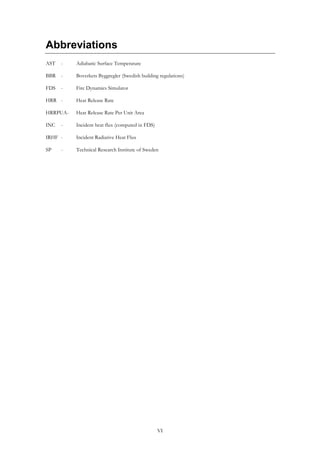
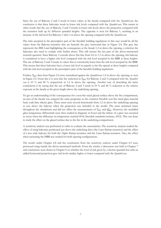
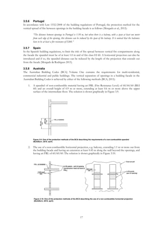
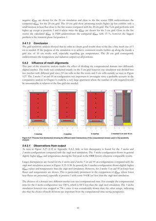
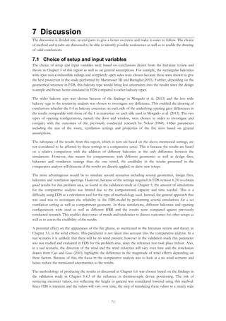
5.1.3 HRR
The produced HRR-curve from the reference test in Evergren et al. (2014) and the same curve produced
using a 10 s moving average are seen in Figure 5.4.
As seen in Figure 5.4, the HRR peaked at 1 800 kW after around 400 s then declined to around 1 500 kW the
following minutes. At around 600 s the fire developed rapidly creating a second peak at approximately 3 000
kW which lasted for about 120 s before it gradually declined as the level of heptane in the trays decreased.
Evergren et al. (2014) describes that a possible explanation for the rapid development between the two
phases could be the heptane starting to boil as the heat in the fire room reaches a significant level. The reason
for the rapid increase in HRR rate could then be this combined effect causing an intensive pyrolysis and
combustion of heptane. Due to defective measurements of HRR in the early stage of the fire the initiation of
the fire was set later in the construction of Figure 5.4. This resulted in a fire scenario of 1 160 s in total.
5.1.4 Recorded temperatures
In Figure 5.5-5.6 the temperatures retrieved from the thermocouples and thermometers during the reference
test in Evergren et al. (2014) are shown at heights as per the marked positions in Figure 5.3.
As indicated by the vertical lines in Figure 5.5, two of the thermocouples (C27 and C28) failed during the test.
The temperatures from both instrument types showed fluctuating behaviour and thus Figure 5.5 and Figure
5.6 are produced using a 30 s moving average.
0
500
1000
1500
2000
2500
3000
3500
0 200 400 600 800 1000 1200
HRR[kW]
Time [s]
Recorded HRR
Figure 5.4: HRR story of the reference test in Evergren et al. (2014). The left picture shows the recorded HRR and the right picture the
recorded HRR using a 10 s moving average to smooth out the data fluctuations.
0
500
1000
1500
2000
2500
3000
3500
0 200 400 600 800 1000 1200
HRR[kW]
Time [s]
HRR using a 10 s moving average
0
100
200
300
400
500
600
700
800
900
0 200 400 600 800 1000 1200
Temperature[ºC]
Time [s]
C21 EXP C22 EXP C23 EXP
C24 EXP C25 EXP C26 EXP
0
100
200
300
400
500
600
700
800
900
1000
0 200 400 600 800 1000 1200
Temperature[ºC]
Time [s]
C27 EXP C28 EXP C29 EXP
C30 EXP C31 EXP C32 EXP
Figure 5.6: Surface temperature measurements during the
reference test at different heights along the facade retrieved
from Inconel steel plate thermocouples.
Figure 5.5: Gas temperature measurements during the reference
test at different heights along the facade retrieved from sheathed
type K thermocouples.](https://image.slidesharecdn.com/b9c25bc4-7009-433b-9915-9df65ba0719b-160222143636/85/Report_5510_Markus_Nilsson-40-320.jpg)
![29
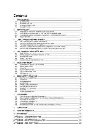
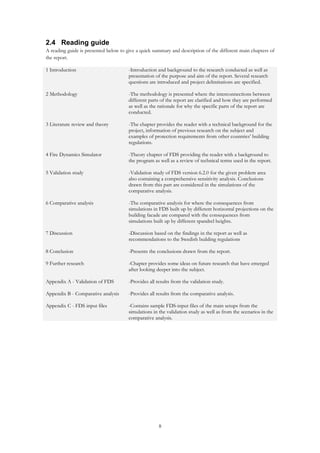
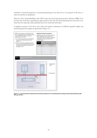
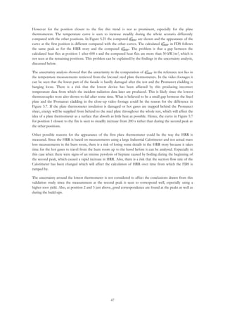
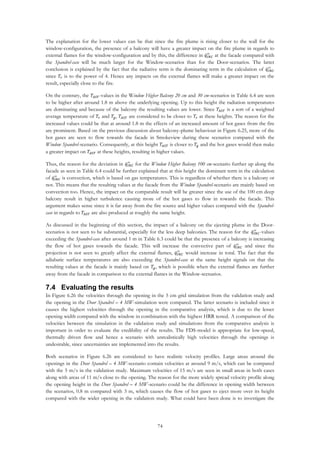
5.1.5 Incident radiation
The incident radiation during the experiment was investigated using the surface temperature measurements
from the Inconel steel plates along the symmetry line of the facade and the gas temperatures retrieved from
the thermocouples. The incident radiation 𝑞̇ 𝐼𝑁𝐶_𝐸
′′
(W/m2) was then derived from the following equation, Eq.
5.1, found in Evergren et al. (2014):
𝑞̇ 𝐼𝑁𝐶_𝐸
′′
= 𝜎𝑇𝑠
4
−
ℎ 𝑐(𝑇𝑔−𝑇𝑠)
𝜀
+
𝑑𝑐𝜌
𝜀
∙
𝑑𝑇
𝑑𝑡
(5.1)
where 𝜎 is the Stefan Boltzmann constant (5.67·10-8 W/[m2·K4]), 𝑑 is the plate thickness (0.7 mm), 𝑐 is the
specific heat of steel (7 850 J/[kg·K]), ρ is the density of the steel plate (480 kg/m3) and 𝜀 is the emissivity
assumed to be of 0.9 [-] (Evergren et al., 2014). The variable 𝑇𝑠 is defined as the surface temperature of the
plate thermometer and 𝑇𝑔 is defined as the temperature of the free air flow (gas temperature). The forced
convective heat transfer coefficient, ℎ 𝑐 (W/[m2·K]), was estimated by the expression in the following
equation, Eq. 5.2 (Evergren et al., 2014):
ℎ 𝑐 = 2.4𝑇𝑓
0.085
∙ 𝑢∞
1/2
∙ 𝑥−1/2
(5.2)
where 𝑢 is the velocity of the vertical air flow and 𝑥 is a characteristic length. Based on video recordings from
the experiment the air velocity was estimated to 6 m/s and the characteristic length was set to 0.2 m (the side
measurement of the square plate). The film temperature 𝑇𝑓 is the average of the 𝑇𝑠 and 𝑇𝑔 (Evergren et al.,
2014). The resulting forced convective heat transfer coefficient ℎ 𝑐 at the various positions varied between 22
and 24 using equation 5.2.
Equation 5.1 is created using the simplified heat balance equation, Equation 289, in Wickström (2015) as a
basis. The heat balance equation describes the heat balance on the exposed plate surface of a plate
thermometer. The term 𝑞̇ 𝐼𝑁𝐶
′′
to the left is extracted from the heat balance equation and the heat loss through
conduction is neglected. However, the convective term is subtracted from the equation. This means, in other
words, that 𝑞̇ 𝐼𝑁𝐶_𝐸
′′
is the incident radiative part of the total heat transfer hence this output is referred to as
incident radiative heat flux, 𝑞̇ 𝐼𝑅𝐻𝐹
′′
(W/m2), in this report.
With equation 5.1 and 5.2 the 𝑞̇ 𝐼𝑅𝐻𝐹
′′
at the facade could be determined along the height of the facade at six
positions as per Figure 5.3. The results are presented in Figure 5.7-5.8.
Figure 5.7: Computed incident radiative heat fluxes to the facade
close to the opening during the reference test.
Figure 5.8: Computed incident radiative heat fluxes to the facade
further up during the reference test.
0
10
20
30
40
50
60
70
80
90
0 200 400 600 800 1000 1200
Incidentradiativeheatflux[kW/m2]
Time [s]
q_IRHF 1 q_IRHF 2 q_IRHF 3
0
0.5
1
1.5
2
2.5
3
3.5
4
4.5
0 200 400 600 800 1000 1200
Incidentradiativeheatflux[kW/m2]
Time [s]
q_IRHF 4 q_IRHF 5 q_IRHF 6](https://image.slidesharecdn.com/b9c25bc4-7009-433b-9915-9df65ba0719b-160222143636/85/Report_5510_Markus_Nilsson-41-320.jpg)
![30
5.1.6 Fire development
During the experiment pictures were taken showing the fire development over time for the heptane fire. The
pictures are presented in Figure 5.9 together with their split times.
5.2 Validation of FDS
In this Section, the simulation setup for the main FDS-simulations is presented. An FDS input file
representing the 5 cm grid setup on a single mesh is shown in Appendix C.1.
5.2.1 Computational domain
The FDS-simulations were performed at three different grid sizes as seen in Table 5.1.
Table 5.1: Various measurements of the computational domain in FDS
Grid size [cm] Domain size Total number of cells Mesh resolution 𝑫∗
/𝜹𝒙
5 4 m (W) * 3.6 m (D) * 7.2 m (H) 829 440 30
10 4 m (W) * 3.6 m (D) * 7.2 m (H) 103 680 15
20 3.8 m (W) * 3.8 m (D) * 7.4 m (H) 13357 8
These simulations were built up by a single mesh, hence resulting in longer simulation times than for a
domain built up by multiple meshes. However, there is a risk that the mesh alignments affect the calculations
in FDS if they are placed in sensitive areas. This in turn can bring further uncertainties to the results. Because
of this, primary results from FDS for this validation study will be based on the single mesh calculations for
the grid sizes according to Table 5.1. In Chapter 5.4 of this report a sensitivity analysis is conducted covering
the potential influence on results of different mesh alignments.
As seen in Table 5.1, the ratio 𝐷∗
/𝛿𝑥 for the conducted simulations are approximately 8, 15 and 30 for the
coarse, medium and fine grid respectively. These values can be compared with the range of 4-16 as
mentioned in the theory in Chapter 4.3. In this case the fine grid size of 5 cm corresponds to a higher value
than 16, which means it is considered to give better results from the accuracy perspective but however less
from the simulation time perspective.
5.2.2 Design fire
The design fire in FDS is based on the chemical properties of heptane and the HRR measurements from the
large Industrial Calorimeter during the reference test. Because of the use of a flame suppressing lattice in the
large-scale fire test, the design fire in FDS cannot be modelled by letting FDS predict the HRR as a heptane
pool fire, since the HRR in the latter case would have been higher without the flame suppressing lattice.
Instead, the HRR measurements collected from the reference test were used to model the HRR-curve for a
surface with a specified HRRPUA using the Ramp Function in FDS.
t = 0 s t = 240 s t = 600 s t = 780 s
Figure 5.9: Pictures showing the fire development during the reference test in Evergren et al. (2014).](https://image.slidesharecdn.com/b9c25bc4-7009-433b-9915-9df65ba0719b-160222143636/85/Report_5510_Markus_Nilsson-42-320.jpg)

![32
5.2.3.1 Building materials
A list of building materials and the thermal properties used in the FDS-simulations are presented in Table 5.2.
Table 5.2: List of materials used in the FDS-simulations during the validation study and their specified thermal properties4
Material Specific heat
[kJ/KgK]
Conductivity
[W/mK]
Density
[kg/m
3
]
Emissivity
[-]
Steel 0.5 48 7800 0.9
Lightweight concrete 1.0 0.15 500 0.9
Promatect 0.975 0.242 1000 0.9
Concrete 1.0 Ramp function* 2300 0.9
Floor insulation 0.479 Ramp function* 140 0.9
Plate insulation Ramp function* Ramp function* 280 0.9
Plate thermometer Ramp function* Ramp function* 8430 0.8
*Ramp function specified in FDS input file in Appendix C.1
Steel was used as material parameter for the burner and concrete as material parameter for the floor. The
building material for the test rig was specified as lightweight concrete and the facade as Promatect.
5.2.4 Measurements
Measurements in FDS during the simulations were collected using slice files and devices for different types of
quantities. In this subsection, the positions and other properties of the measurements are described.
5.2.4.1 Devices
The devices used in the simulation were specified to output temperature and different kind of heat fluxes in
order to obtain comparable results as in Chapter 5.1.4 and 5.1.5. In Figure 5.1, the device positions are shown
in the FDS-model.
The thermocouples used in the simulations were specified to match the sheathed type K thermocouples in
the actual fire test (C27-C32). The default thermocouples in FDS were used as a basis, which is a
nickel/based thermocouple with specific heat of 0.44 kJ/KgK, density of 8908 kg/m3 and emissivity of 0.85.
4Johan Anderson, Research Scientist at SP, e-mail communication 22nd of September 2015
1. Inconel steel plate sheet (C21-C26)
2. Wall temperature device (C21-C26)
3. Thermocouple device as per position in drawing (C27-C32)
4. Thermocouple devices offset symmetry line (Sufix -1 to -10)
5. Velocity measurement device
6. Incident heat flux device
7. Convective heat flux device
8. Adiabatic surface temperature device
9. Oxygen level measurements
1
1
1
1
1
1
1
1
2, 6, 7, 8
3 4
5
3
4
1 m
2, 6, 7, 8
5
9
9
Figure 5.11: Picture showing device positions in FDS for the 5 cm grid simulation. The picture to the left shows the front of the test rig
along with the six thermometers. The middle picture is a close-up of the latter, which is also illustrated in 3D in the picture on the far
right.](https://image.slidesharecdn.com/b9c25bc4-7009-433b-9915-9df65ba0719b-160222143636/85/Report_5510_Markus_Nilsson-44-320.jpg)


![35
5.3 Results
This section presents output data from the main simulations performed on a single mesh. The results in this
subsection are referring to all the results found in Appendix A. Some of the graphs presented are modified to
clarify the results or to highlight important aspects. Data values named EXP are values retrieved from the
reference test and the data values named FDS are those retrieved from the FDS-simulations.
5.3.1 HRR and oxygen levels
In Figure 5.13 the modelled HRR in FDS for the 20, 10 and 5 cm grid simulation are presented.
Figure 5.13: Actual HRR in FDS for the 20, 10 and 5 cm grid simulations.
As seen in Figure 5.13, the fluctuations are decreasing the finer the grid becomes. The fluctuating behaviour
is as largest during the second peak of the fire scenario. The oxygen levels in the air at two positions during
the 5 cm grid simulation are shown in Figure 5.14.
Figure 5.14: Oxygen levels in the air at two positions during the 5 cm grid simulation.
In Figure 5.14, a fluctuating behaviour is seen above the fire at ceiling level between 1-4 percent oxygen
during the first peak. After this, the values are decreasing to zero percent oxygen during the second peak of
the test. At the opening, oxygen levels are varying between 12-14 percent during both peaks.
0
5
10
15
20
25
0 200 400 600 800 1000
Availableoxygen[%]
Time [s]
Above fire Opening
0
400
800
1200
1600
2000
2400
2800
3200
3600
0 200 400 600 800 1000
HRR[kW]
Time [s]
FDS 5 cm
0
400
800
1200
1600
2000
2400
2800
3200
3600
0 200 400 600 800 1000
HRR[kW]
Time [s]
FDS 10 cm
0
400
800
1200
1600
2000
2400
2800
3200
3600
0 200 400 600 800 1000
HRR[kW]
Time [s]
FDS 20 cm](https://image.slidesharecdn.com/b9c25bc4-7009-433b-9915-9df65ba0719b-160222143636/85/Report_5510_Markus_Nilsson-47-320.jpg)
![36
5.3.2 Temperature
In Figure 5.15-5.16, comparisons of the gas temperature data retrieved from the thermocouples in the
reference test and FDS are presented for the 5 cm grid simulation on different heights along the facade.
As seen in Figure 5.15-5.16 a good correspondence is found close to the fire source but FDS slightly
overestimates the temperatures further up, particularly at position C29. This behaviour is fairly consistent for
both peaks during the HRR history.
The same correspondence is not found close to the opening for the 20 cm and 10 cm grid simulation, as seen
in Figure A.1-A.2 and Figure A.5-A.6 in Appendix A.1. The 20 cm grid consistently underestimates the gas
temperatures at all heights during the whole HRR history. The 10 cm grid underestimates the temperatures at
position C27 and C28.
At the position closest to the fire, C27, temperatures 300 C less than actual are produced at both peaks. At
position C28, a good correspondence is found at the first peak but underestimating the temperature with
some 200 C at the second peak. A good temperature representation is seen at position C29-C32 for the 10
cm grid. In Figure 5.17-5.18, comparisons of the surface temperature data retrieved from the thermometers
in the reference test and FDS are presented for the 5 cm grid simulation on different heights along the
facade.
A good agreement is seen at position C23-C26 except for a slight underestimation at position C25 and C26 as
well as for a slight overestimation at position C23 and C24. An underestimation of some 100 C can be found
0
50
100
150
200
250
300
350
400
450
500
0 200 400 600 800 1000 1200
Temperature[ºC]
Time [s]
C30 EXP C31 EXP C32 EXP
C30 FDS C31 FDS C32 FDS
Figure 5.15: FDS 5 cm cells, comparison of gas temperature during
the reference test and those calculated in FDS for the sheathed type
K thermocouples close to the opening.
Figure 5.16: FDS 5 cm cells, comparison of gas temperature during
the reference test and those calculated in FDS for the sheathed
type K thermocouples further up along the facade.
0
100
200
300
400
500
600
700
800
900
1000
0 200 400 600 800 1000 1200
Temperature[ºC]
Time [s]
C27 EXP C28 EXP C29 EXP
C27 FDS C28 FDS C29 FDS
Figure 5.17: FDS 5 cm cells, comparison of surface temperature
during the reference test and those calculated in FDS for the Inconel
steel plate thermometers close to the opening.
Figure 5.18: FDS 5 cm cells, comparison of surface temperature
during the reference test and those calculated in FDS for the
Inconel steel plate thermometers further up along the facade.
0
50
100
150
200
250
300
0 200 400 600 800 1000 1200
Surfacetemperature[ºC]
Time [s]
C24 EXP C25 EXP C26 EXP
C24 FDS C25 FDS C26 FDS
0
100
200
300
400
500
600
700
800
900
0 200 400 600 800 1000 1200
Surfacetemperature[ºC]
Time [s]
C21 EXP C22 EXP C23 EXP
C21 FDS C22 FDS C23 FDS](https://image.slidesharecdn.com/b9c25bc4-7009-433b-9915-9df65ba0719b-160222143636/85/Report_5510_Markus_Nilsson-48-320.jpg)
![37
at position C28 closer to the fire. However, closest to the fire the modelled plate thermometers have
problems to produce correct transient temperatures in the early stage of the fire but in the second peak it
underestimates the temperature with some 100 C.
As for the 20 cm and 10 cm grid simulations found in Appendix A.1, temperature underestimations of
different sizes are seen. The 20 cm grid heavily underestimates the temperatures on all heights whereas in the
10 cm grid simulation there is a general trend of less underestimation the further up the facade that FDS
measures. Closest to the fire though, the 10 cm grid simulation calculate temperatures some 300 C less than
actual measurements.
In general, FDS version 6.2.0 seems to produce higher temperatures on all positions than in FDS version
5.5.3 based on comparisons to the validations study performed by Anderson and Jansson (2013), especially
the temperatures retrieved from the modelled plate thermometers.
5.3.3 Adiabatic surface temperature
In Figure 5.19-5.20, a comparison of 𝑇𝐴𝑆𝑇 in FDS and the retrieved surface temperatures from the
thermometers during the reference test are shown for the 5 cm grid.
Unlike the already discussed modelled thermometers in Figure 5.17-5.18, the 𝑇𝐴𝑆𝑇-values are slightly
overestimating the surface temperatures retrieved from the thermometers at position C22-C26 for the 5 cm
grid. At position C21, the transient representation of the temperature rise is better represented in this
simulation and just underestimating the actual measurements at the second peak. From Appendix A.2 it can
be seen that the 20 cm grid consistently generate lower temperatures than actual and for the 10 cm grid a
good correspondence is found at position C23-C26. However, at position C21 and C22 FDS consistently
generate lower temperatures than actual measurements for the 10 cm grid.
0
50
100
150
200
250
300
350
400
0 200 400 600 800 1000 1200
Surfacetemperature[ºC]
Time [s]
C24 EXP C25 EXP C26 EXP
C24 FDS 5 cm C25 FDS 5 cm C26 FDS 5 cm
Figure 5.19: Comparison of surface temperatures retrieved from the
Inconel thermometers and adiabatic surface temperatures from FDS
close to the opening during the reference test.
Figure 5.20: Comparison of surface temperatures retrieved from
the Inconel thermometers and adiabatic surface temperatures
from FDS further up along the facade during the reference test.
0
100
200
300
400
500
600
700
800
900
0 200 400 600 800 1000 1200
Surfacetemperature[ºC]
Time [s]
C21 EXP C22 EXP
C23 EXP C21 FDS 5 cm
C22 FDS 5 cm C23 FDS 5 cm](https://image.slidesharecdn.com/b9c25bc4-7009-433b-9915-9df65ba0719b-160222143636/85/Report_5510_Markus_Nilsson-49-320.jpg)
![38
5.3.4 Incident radiation
The computed 𝑞̇ 𝐼𝑅𝐻𝐹
′′
at the facade during the reference test and the corresponding measurements in FDS are
shown in Figure 5.21-5.22 for the 5 cm grid simulation.
At position 2 and 5 a good agreement is found between the measurements. At position 3 and 4 however the
𝑞̇ 𝐼𝑅𝐻𝐹
′′
is twice the actual in FDS. A similar behaviour is seen at position 6. At position 1 closest to the fire,
FDS is having trouble to match the computed radiation in the transient approach. However, later on at the
second peak of the HRR story the 𝑞̇ 𝐼𝑅𝐻𝐹
′′
calculated in FDS underestimates the computed 𝑞̇ 𝐼𝑅𝐻𝐹
′′
with some 15
%.
The 20 cm grid simulation has problems matching the computed 𝑞̇ 𝐼𝑅𝐻𝐹
′′
as seen in Figure A.15-A.16 in
Appendix A.3, especially further up where negative values are produced. The 10 cm grid shows good
correspondence at position 3,4,5 and 6 but underestimates 𝑞̇ 𝐼𝑅𝐻𝐹
′′
at position 1 and 2 significantly.
In general, FDS version 6.2.0 seems to produce higher 𝑞̇ 𝐼𝑅𝐻𝐹
′′
-values on all positions than in FDS version 5.5.3
based on comparisons to the validations study performed by Anderson and Jansson (2013).
5.3.5 External flames
To predict the appearance of the external flames in FDS, pictures of the heat release rate per unit volume
were rendered from Smokeview, which gives an indication of the location of the combustion reaction. As
seen in Figure 5.23, a realistic picture of external flames is produced in the 10 cm grid simulation compared
with the 20 cm grid. The appearance of external flames for the 5 cm grid is more realistic though; having a
greater vertical reach which better corresponds to the reference test to the right. There is a small tendency of
a too narrow appearance of flames in the 5 cm grid compared with the actual flames.
Figure 5.21: FDS 5 cm cells, comparison of calculated incident
radiative heat flux and those computed by FDS close to the opening
during the reference test.
Figure 5.22: FDS 5 cm cells, comparison of calculated incident
radiative heat flux and those computed by FDS further up
along the facade during the reference test.
0
10
20
30
40
50
60
70
80
90
0 200 400 600 800 1000 1200
Incidentradiativeheatflux[kW/m2]
Time [s]
q_IRHF 1 q_IRHF 2 q_IRHF 3
FDS IRHF 1 FDS IRHF 2 FDS IRHF 3
0
2
4
6
8
10
0 200 400 600 800 1000 1200
Incidentradiativeheatflux[kW/m2]
Time [s]
q_IRHF 4 q_IRHF 5 q_IRHF 6
FDS IRHF 4 FDS IRHF 5 FDS IRHF 6
20 cm grid 10 cm grid 5 cm grid Reference test
Figure 5.23: Comparison of external flames in the FDS-simulations and the reference test at approximately 600 s.](https://image.slidesharecdn.com/b9c25bc4-7009-433b-9915-9df65ba0719b-160222143636/85/Report_5510_Markus_Nilsson-50-320.jpg)

![40
5.4 Sensitivity analysis
This section of the report is divided into seven subsections. The first subsection concerns the sensitivity in
the choice of grid size, the second subsection concerns the influence of different mesh alignments and the
third subsection presents the sensitivity in the choice of position of thermocouple devices in the simulation.
The following three subsections describe the sensitivity in the choice of radiation angles, the sensitivity in the
choice of HRRPUA as well as the sensitivity in the choice of soot yield. The last subsection is an overall
conclusion of the sensitivity study performed.
5.4.1 Grid sensitivity
The foundations of this grid sensitivity analysis can be seen in Appendix A.2 and A.4 where several graphs
and pictures are presented. In Figure 5.26, a transient representation of the mesh resolution is shown for the
coarse, medium as well as for the fine grid size.
Figure 5.26: Transient representation of the calculated 𝑫∗
/𝜹𝒙 for the fine, medium and coarse grid for the reference test simulations.
As previously been stated in the theory in Chapter 4.3 of this report, the ratio between 𝐷∗
and 𝛿𝑥 should be
between 4 and 16 according to McGrattan et al. (2015). The grid sizes used in these simulations result in
ratios of around 8, 15 and 30 for the 20, 10 and 5 cm simulation at maximum HRR 3.1 MW, which are well
within and even above the recommended ratio. In Figure 5.26 it can be seen that the coarse simulation and
fine simulation reaches the proposed value of 4 and 16 after around 180 s. Hence, all the simulations are
within the accepted range mentioned in Chapter 4.3 during both peaks in the HRR story, where the fine grid
size has a larger value than 16.
However, a finer grid resolution results in higher computational cost, which also has to be considered when
setting up FDS-simulations. For the current single mesh simulations, computational times of 1.5, 18 and 232
h were exhibited for the 20, 10 and 5 cm cells.
5.4.1.1 Observations from output – Temperatures
As seen in Figure A.13-A.14 in Appendix A.2 and A.21-A.24 in Appendix A.4.1, the overall difference
between the coarse grid size and the other grid sizes are large regarding devices measuring 𝑇𝐴𝑆𝑇,
thermocouples as well as for temperatures from thermometers. The 20 cm grid size does not only have
problems reaching the retrieved temperatures close to the fire, but also higher up the coarse grid size
consequently underestimates the actual temperatures. The 10 cm grid performs well at positions further up
along the facade in general, however close to the fire source large discrepancies are found. The 5 cm grid
performs well close to the fire source in general but slightly overestimates the temperatures further up along
the facade retrieved from the thermocouples and devices measuring 𝑇𝐴𝑆𝑇. Most problems can be seen in the
transient phase before the first and second peak in HRR for the modelled thermometers and 𝑇𝐴𝑆𝑇. In this
instance, 𝑇𝐴𝑆𝑇 performs better.
5.4.1.2 Observations from output – Incident radiation
Similar to the temperature outputs, the overall difference between the coarse grid size and the other grid sizes
are large in regards to 𝑞̇ 𝐼𝑅𝐻𝐹
′′
as seen in Figure A.25-A.26 in Appendix A.4.1. At position four, five and six
0
5
10
15
20
25
30
35
0 200 400 600 800 1000 1200
D*/δx[-]
Time [s]
Fine Medium Coarse](https://image.slidesharecdn.com/b9c25bc4-7009-433b-9915-9df65ba0719b-160222143636/85/Report_5510_Markus_Nilsson-52-320.jpg)


![44
input parameters, which has been investigated further. This could impact the validity of the computed 𝑞̇ 𝐼𝑅𝐻𝐹
′′
that are used as results in the validation study.
Initially, the velocity parameter in the convective heat transfer coefficient was investigated since the
calculations in Evergren et al. (2014) only used a constant value estimated from video recordings. This was
done using numerical estimated velocity data from devices in the 5 cm grid simulation on a single mesh and
then implemented in the equation for the convective heat transfer coefficient. The devices were positioned
just outside the plate thermometers as seen in Figure 5.11. In Figure 5.28-5.29, the 𝑞̇ 𝐼𝑅𝐻𝐹
′′
is compared
between the cases.
The results in Figure 5.28-5.29 indicate that the change in velocity parameter made little or no impact on the
radiation output. The convective heat transfer coefficients based on a constant velocity used in the
calculations varies between 22-24 W/(m2·K). This range of values can be set in relation to the recommended
value of 25 W/(m2·K) stated by Buchanan H. (2002). Buchanan H. (2002) also states that in typical fires, heat
transfer is not very sensitive to this value since radiative heat transfer is the dominating factor. The latter is
also recognized by Wickström (2015).
To study the significance of the convective heat transfer term (second term to the right) as well as the rate of
heat stored in the plate (the far right term) in equation 5.1, a comparison was made between the calculated
𝑞̇ 𝐼𝑅𝐻𝐹
′′
as per equation 5.1 and the heat flux calculated only by the first term in in the equation. The results are
shown in Figure 5.30-5.31.
Figure 5.28: Comparison of different incident radiative heat fluxes
close to the opening during the reference test. Heat fluxes
produced either by assuming a constant gas velocity or by using
numerical estimated transient velocities (suffix –v).
Figure 5.29: Comparison of different incident radiative heat
fluxes further up along the facade during the reference test.
Heat fluxes produced either by assuming a constant gas
velocity or by using numerical estimated transient velocities
(suffix –v).
0
10
20
30
40
50
60
70
80
90
0 200 400 600 800 1000 1200
Incidentradiativeheatflux[kW/m2]
Time [s]
qinc1 qinc2 qinc3
qinc1 v qinc2 v qinc3 v
0
1
2
3
4
5
0 200 400 600 800 1000 1200Incidentradiativeheatflux[kW/m2]
Time [s]
qinc4 qinc5 qinc6
qinc4 v qinc5 v qinc6 v
Figure 5.30: Comparison of the output incident radiative heat flux as
per equation 5.1 and the output of just the first term (prefix T#) in
equation 5.1, close to the opening during the reference test.
Figure 5.31: Comparison of the output incident radiative heat
flux as per equation 5.1 and the output of just the first term
(prefix T#) in equation 5.1, further up along the facade during the
reference test.
0
10
20
30
40
50
60
70
80
90
0 200 400 600 800 1000 1200
Incidentheatflux[kW/m2]
Time [s]
qinc1 qinc2 qinc3
T4 1 T4 2 T4 3
0
1
2
3
4
5
0 200 400 600 800 1000 1200
Incidentheatflux[kW/m2]
Time [s]
qinc4 qinc5 qinc6
T4 4 T4 5 T46](https://image.slidesharecdn.com/b9c25bc4-7009-433b-9915-9df65ba0719b-160222143636/85/Report_5510_Markus_Nilsson-56-320.jpg)


![52
As seen in Figure 6.6, the balconies were specified the same width as the corresponding opening.
6.2.4 Building materials
A list of building materials and the thermal properties used in the FDS-simulations are presented in Table 6.1.
Table 6.1: List of materials used in the FDS-simulations during the comparative analysis and their specified thermal properties
Material Specific heat
[kJ/KgK]
Conductivity
[W/mK]
Density
[kg/m
3
]
Emissivity
[-]
Absorption
coefficient [m
-1
]
Facade concrete* 1.04 1.8 2280 0.9 Default value in FDS
Concrete 0.0104** 1.8 2280 0.9 Default value in FDS
Basic soda lime silicate glass*** 0.72 1 2500 0.837 500****
*NBSIR 88-3752 - ATF NIST Multi-Floor Validation, FDS Library
**The original specific heat value of concrete divided by a factor of 100
***Thermal properties collected from Swedish standards institute (2012)
****Value collected from Dembele, Rosario, Wen, Warren and Dale (2008)
Concrete was used as material parameter for all the apartment walls, floor and ceiling. The reason for using a
specific heat divided by a factor of 100 in this modified material parameter is explained further in Chapter 6.6.
The material entitled facade concrete was used in the facade of the overlying apartment containing a glazed
surface, which in turn was denoted the material basic soda lime silicate glass. The backside boundary
condition BACKING='VOID' was set to the building material surface for all the apartment walls, floor and ceiling,
except for the facade where the condition BACKING='EXPOSED' was applied. The latter was specified since heat
calculations through the wall in FDS were assumed to occur from both sides of the facade due to the fire
plume ejecting from the opening in the facade.
6.3 Measurements
Measurements in FDS during the simulations were collected using slice files and devices for different types of
quantities. In this subsection, the positions and other properties of the measurements are described.
6.3.1 Devices
In Figure 6.7, the device positions are shown in the FDS-model for the Door Spandrel-scenarios.
As seen in the middle picture in Figure 6.7, devices measuring 𝑇𝐴𝑆𝑇 and 𝑞̇ 𝐼𝑁𝐶
′′
were placed in each cell at the
facade, starting just above the door and ending 3.2 m above. The reason for the measurements ending at this
height is the assumption of a similar door positioned in a compartment above with a 1.2 spandrel as per the
BBR. In total, 16 devices were included in each row with a total of 64 rows along the height, covering an area
of 0.8 (W) * 3.2 (H) m2 of the facade above. The window configuration was designed in the same way as in
Figure 6.7 however because the window is wider than the door, 24 devices were placed in each row.
1, 2
3
4
1, 2
3.2m
1. Adiabatic surface temperature devices
2. Incident heat flux devices
3. Door thermocouples
4. Wall temperature measurements
5. Oxygen level measurements
6. Thermocouple tree (3 devices in height)
Front of the fire compartment Fire compartment seen from above
5, door5, above fire
6
1, 2, 3, 4
Figure 6.7: Picture showing device positions in FDS for the Door Spandrel-scenarios. The picture to the left shows the front of the
compartment where the middle picture is a close-up of the latter. The picture on the far right illustrates the device positions in the
compartment seen from above.](https://image.slidesharecdn.com/b9c25bc4-7009-433b-9915-9df65ba0719b-160222143636/85/Report_5510_Markus_Nilsson-64-320.jpg)

![54
combustion as the weighted value of 40 mass percent of polyurethane and 60 mass percent of wood (BIV,
2013).
To avoid numerical instability the fire was ramped up to maximum HRR over 10 s from where it continued
throughout the simulation. A HRRPUA of 3100 kW/m2 on a 1 m2 burner resulted in a maximum HRR of
3.1 MW for the main simulations. Using Equation 5.24 in Karlsson and Quintiere (2000), the maximum HRR
for the Door- and Window-scenarios would be 5.3 MW and 4.1 MW respectively. This is for a fully
developed under-ventilated fire assuming all oxygen entering the room are used for combustion and each
kilogram of oxygen produces 13.2 MJ. The chosen HRR of 3.1 MW is smaller than these values for both
opening configurations and hence considered to be of a less under-ventilated variety, which is considered
favourable since previous research on FDS shows that large errors could occur when performing calculations
during under-ventilated fires (Nystedt & Frantzich, 2011). Also, a HRRPUA of 3100 kW/m2 and a 1 m2
burner was chosen because the same setup were used in the validation study, which enables one to compare
better.
A higher HRR of 4 MW was used for both opening configurations in the sensitivity study to investigate its
effect on the output. As for the Window-scenarios, this HRR is seen nearly as the maximum HRR that could
be obtained in the fire compartment according to Equation 5.24 in Karlsson and Quintiere (2000).
6.5 Miscellaneous settings
In the simulations the following miscellaneous settings were used:
The simulation time was set to 180 s
The ambient temperature was set to 20 ºC
The boundary exterior of the computational domain were set open
6.6 Producing the results
Since FDS is transient and the data values from each device measuring 𝑇𝐴𝑆𝑇 and 𝑞̇ 𝐼𝑁𝐶
′′
seen in Figure 6.7 are
fluctuating over time, it is difficult to describe the damage at the facade in a comparative sense. As already
described in the methodology in Chapter 2 of this report, the goal was to produce graphs of the receiving
𝑇𝐴𝑆𝑇 and 𝑞̇ 𝐼𝑁𝐶
′′
at the facade as a function of the height above the opening. This means only one value at each
height above the opening will be addressed. To do this, the recorded data from the transient phase need to be
reworked.
In Figure 6.9 the recorded data from each device at the first row measuring 𝑇𝐴𝑆𝑇 are shown throughout the
simulation for the Door Spandrel-scenario.
As seen in the example Figure 6.9, the recorded data are at a fairly constant level after 40 s. This is because of
the use of concrete material inside the fire compartment with a specific heat divided by 100, as mentioned in
Figure 6.9: Adiabatic surface temperature data from each device at
the first row for the Door Spandrel-scenario.
Figure 6.10: Adiabatic surface temperature data from each device
as moving average over 10 s at the first row for the Door
Spandrel-scenario.
0
100
200
300
400
500
600
700
800
900
0 20 40 60 80 100 120 140 160 180
Adiabaticsurfacetemperature[ºC]
Time [s]
Dev 1 Dev 2 Dev 3 Dev 4
Dev 5 Dev 6 Dev 7 Dev 8
Dev 9 Dev 10 Dev 11 Dev 12
Dev 13 Dev 14 Dev 15 Dev 16
0
100
200
300
400
500
600
700
800
900
0 20 40 60 80 100 120 140 160 180
Adiabaticsurfacetemperature[ºC]
Time [s]
Dev 1 Dev 2 Dev 3 Dev 4
Dev 5 Dev 6 Dev 7 Dev 8
Dev 9 Dev 10 Dev 11 Dev 12
Dev 13 Dev 14 Dev 15 Dev 16](https://image.slidesharecdn.com/b9c25bc4-7009-433b-9915-9df65ba0719b-160222143636/85/Report_5510_Markus_Nilsson-66-320.jpg)
![55
Chapter 6.2.4. During the iterative work when using normal concrete inside the fire compartment, these lines
were seen to constantly increase which was problematic, since one of the disadvantages with the finer grid
size is the rapid increase in computational time. Using the modified concrete speeds up the heating of the
concrete hence reaching the equilibrium state faster than for normal concrete. Since this procedure is done
for all the simulations and the aim of the report is to compare the Spandrel-case and the scenarios within the
Balcony-case, this is not seen to affect the credibility of the results. On the contrary, this procedure makes it
easier to do the comparative analysis since it is considered to be a single value not expected to increase a lot
more if a longer simulation time was specified. This will increase the credibility of the numbers in the results
in an absolute sense, which makes it easier also to relate to previous research.
The recorded data from each device were averaged over 10 s as a moving average, which is seen in Figure
6.10. This was done to remove some of the fluctuations over time. Since the interrelationship between the
data values from each device over time on every row was seen to be fairly constant, the maximum value
observed from each of the sixteen devices over time was used to describe the damage at the facade for that
specific row over time. In Figure 6.11 the maximum values over time for the specific example in Figure 6.10
are shown.
As seen in Figure 6.11, the data recorded before 10 s was removed since the fire is not reaching its maximum
HRR during these seconds. Lastly, to express the damage at the facade at a specific height without the time-
variable, a mean value was calculated of the curve, as seen in Figure 6.11. This value was then used in the
graph for that specific row and height. Since devices were distributed over 64 rows along the facade above
the opening, data was recorded and results produced following the above procedure at 64 positions.
The approach mentioned above for determining the damage to the facade along the height was used for all
the simulations. The only difference between producing results for the Window-scenarios and Door-
scenarios was that the max value at every row was determined based on the data from 24 devices at every row
instead of 16.
Figure 6.11: Maximum values of the sixteen devices over time at the first row in the Door Spandrel-scenario. The first 10 s are removed
since during these seconds the fire has not reached its maximum HRR.
0
100
200
300
400
500
600
700
800
900
0 20 40 60 80 100 120 140 160 180
Adiabaticsurfacetemperature[ºC]
Time [s]
Max over t Mean value](https://image.slidesharecdn.com/b9c25bc4-7009-433b-9915-9df65ba0719b-160222143636/85/Report_5510_Markus_Nilsson-67-320.jpg)

![57
6.8 Results
The results in this subsection are referring to all the results found in Appendix B. Some of the graphs
presented are modified to clarify the results or to highlight important aspects. The reader is referred to the
methodology in Chapter 2.3 for clarifications of how to read some of the results.
6.8.1 HRR and oxygen levels
In Figure 6.12 the HRR in FDS are presented for the scenarios within the Spandrel-case.
As seen in the figure, there are tendencies for a larger fluctuation in HRR for the Window-scenarios compare
to the Door-scenarios on both HRR-levels. The oxygen levels in the air at two positions for the scenarios
within the Spandrel-case are shown in Figure 6.13.
The results in Figure 6.13 can be compared with the results in Figure 5.14 in the validation study for the 5 cm
grid simulation. As seen in Figure 6.13 the oxygen levels above the fire are between 1-4 percent during the
simulation compared with the zero percent oxygen levels found in Figure 5.14 during the second peak of the
fire in the validation study.
6.8.2 Results from the scenarios within the Spandrel-case
In Figure B.1-B.2 in Appendix B.1 the 𝑇𝐴𝑆𝑇 data and 𝑞̇ 𝐼𝑁𝐶
′′
data are compared between the scenarios within the
Spandrel-case. In the figures it is seen that the values obtained from the 4 MW-scenarios are higher than each
of the values of the corresponding scenarios performed on a lower HRR. It is also seen that the values
obtained from the Window-scenarios are higher than each of the values from the corresponding Door-
scenarios.
0.0
0.5
1.0
1.5
2.0
2.5
3.0
3.5
4.0
4.5
5.0
0 90 180
HRR[MW]
Time [s]
HRR Door Spandrel
Figure 6.12: HRR story from the scenarios within the Spandrel-case.
0.0
0.5
1.0
1.5
2.0
2.5
3.0
3.5
4.0
4.5
5.0
0 90 180
HRR[MW]
Time [s]
HRR Door Spandrel – 4 MW
0.0
0.5
1.0
1.5
2.0
2.5
3.0
3.5
4.0
4.5
5.0
0 90 180
HRR[MW]
Time [s]
HRR Window Spandrel
0.0
0.5
1.0
1.5
2.0
2.5
3.0
3.5
4.0
4.5
5.0
0 90 180
HRR[MW]
Time [s]
HRR Window Spandrel – 4
MW
Figure 6.13: Oxygen levels in the air at two positions for the scenarios within the Spandrel-case.
0
5
10
15
20
25
0 90 180
Availableoxygen[%]
Time [s]
Door Spandrel
Above fire
Door
0
5
10
15
20
25
0 90 180
Availableoxygen[%]
Time [s]
Window Spandrel
Above fire
Window
0
5
10
15
20
25
0 90 180
Availableoxygen[%]
Time [s]
Door Spandrel- 4 MW
Above fire
Door
0
5
10
15
20
25
0 90 180
Availableoxygen[%]
Time [s]
Window Spandrel - 4 MW
Above fire
Window](https://image.slidesharecdn.com/b9c25bc4-7009-433b-9915-9df65ba0719b-160222143636/85/Report_5510_Markus_Nilsson-69-320.jpg)
![58
6.8.3 Results from the Door Higher Balcony-scenarios
In Figure 6.14 the external flames from the Door Spandrel-scenario and the Door Higher Balcony-scenarios are
compared.
From Figure 6.14 an airgap between the balcony and the fire plume is visible for all the scenarios. For the 100
cm deep balcony it is seen that the outer part of the balcony is in contact with the plume.
In Figure 6.15-6.16, comparisons of 𝑇𝐴𝑆𝑇 data and 𝑞̇ 𝐼𝑁𝐶
′′
data are made between the Door Spandrel-scenario and
the Door Higher Balcony-scenarios. As seen in Figure 6.15-6.16, the measurements presented in the diagrams
start at 0.6 m due to the presence of balconies at 0.35-0.55 m above the door for the Door Higher Balcony-
scenarios.
50
100
150
200
250
300
350
400
0.6 0.8 1 1.2 1.4 1.6 1.8 2 2.2 2.4 2.6 2.8 3 3.2
Adiabaticsurfacetemperature[ºC]
Height above door [m]
AST Door Spandrel AST BBR Limit AST Door Higher Balcony 20 cm
AST Door Higher Balcony 30 cm AST Door Higher Balcony 60 cm AST Door Higher Balcony 80 cm
AST Door Higher Balcony 100 cm
Figure 6.15: A comparison of the adiabatic surface temperature at the facade above the door at different heights between the Door Spandrel-
scenario and the Door Higher Balcony-scenarios
Figure 6.14: A comparison of the external flames between the Door Spandrel-scenario and the Door Higher Balcony-scenarios.
Door Spandrel Door Higher Balcony
20 cm
Door Higher Balcony
30 cm
Door Higher Balcony
60 cm
Door Higher Balcony
80 cm
Door Higher Balcony
100 cm](https://image.slidesharecdn.com/b9c25bc4-7009-433b-9915-9df65ba0719b-160222143636/85/Report_5510_Markus_Nilsson-70-320.jpg)
![59
In Figure 6.17-6.18, the 𝑇𝐴𝑆𝑇 data and 𝑞̇ 𝐼𝑁𝐶
′′
data from the Door Higher Balcony-scenarios are normalized against
the Spandrel-case 1.2 m above the door.
1
2
3
4
5
6
7
8
9
10
11
12
13
14
0.6 0.8 1 1.2 1.4 1.6 1.8 2 2.2 2.4 2.6 2.8 3 3.2
Incidentheatflux[kW/m2]
Height above door [m]
INC Door Spandrel INC BBR Limit INC Door Higher Balcony 20 cm
INC Door Higher Balcony 30 cm INC Door Higher Balcony 60 cm INC Door Higher Balcony 80 cm
INC Door Higher Balcony 100 cm
Figure 6.16: A comparison of the incident heat flux at the facade above the door at different heights between the Door Spandrel-scenario
and the Door Higher Balcony-scenarios
0.3
0.4
0.5
0.6
0.7
0.8
0.9
1
1.1
1.2
1.3
1.4
1.5
1.6
0.6 0.8 1 1.2 1.4 1.6 1.8 2 2.2 2.4 2.6 2.8 3 3.2
Relativeexposure[-]
Height above door [m]
AST Door Spandrel AST Door Higher Balcony 20 cm AST Door Higher Balcony 30 cm
AST Door Higher Balcony 60 cm AST Door Higher Balcony 80 cm AST Door Higher Balcony 100 cm
Figure 6.17: A comparison between the Door Spandrel-scenario and the Door Higher Balcony-scenarios using adiabatic surface temperature
data normalized against the Spandrel-case 1.2 m above the door. The point of origin for the normalization is highlighted as a cross on the
Spandrel-case line.](https://image.slidesharecdn.com/b9c25bc4-7009-433b-9915-9df65ba0719b-160222143636/85/Report_5510_Markus_Nilsson-71-320.jpg)
![60
In Table 6.3, a summary of the key results are shown observed from the graphs above.
Table 6.3: Summary of the key results observed from Figure 6.15-6.18 for the Door Higher Balcony-scenarios
Proxy
variable
Criteria Door Higher
Balcony 20
cm
Door Higher
Balcony 30
cm
Door Higher
Balcony 60
cm
Door Higher
Balcony 80
cm
Door
Higher
Balcony
100 cm
Adiabatic
surface
temperature
Values lower than the Door
Spandrel-scenario
No, values
exceeding
after 1.0 m
Yes Yes Yes Yes
Risk level compared with the
Door Spandrel-scenario
Higher, after
1.0 m
Lower Lower Lower Lower
Risk level compared with the
one accepted in the
prescriptive part of the BBR
Higher Lower Lower Lower Lower
Reduction/increase in the
relative exposure at 1.2 m
above the underlying door
+5 % -10 % -20 % -30 % -40 %
Incident heat
flux
Values lower than the Door
Spandrel-scenario
No, values
exceeding
after 1.05 m
Yes Yes Yes Yes
Risk level compared with the
Door Spandrel-scenario
Higher, after
1.05 m
Lower Lower Lower Lower
Risk level compared with the
one accepted in the
prescriptive part of the BBR
Higher Lower Lower Lower Lower
Reduction/increase in the
relative exposure at 1.2 m
above the underlying door
+5 % -20 % -35 % -45 % -60 %
0.1
0.2
0.3
0.4
0.5
0.6
0.7
0.8
0.9
1
1.1
1.2
1.3
1.4
1.5
1.6
1.7
1.8
1.9
2
2.1
2.2
2.3
0.6 0.8 1 1.2 1.4 1.6 1.8 2 2.2 2.4 2.6 2.8 3 3.2
Relativeexposure[-]
Height above door [m]
INC Door Spandrel INC Door Higher Balcony 20 cm INC Door Higher Balcony 30 cm
INC Door Higher Balcony 60 cm INC Door Higher Balcony 80 cm INC Door Higher Balcony 100 cm
Figure 6.18: A comparison between the Door Spandrel-scenario and the Door Higher Balcony-scenarios using incident heat flux data
normalized against the Spandrel-case 1.2 m above the door. The point of origin for the normalization is highlighted as a cross on the
Spandrel-case line.](https://image.slidesharecdn.com/b9c25bc4-7009-433b-9915-9df65ba0719b-160222143636/85/Report_5510_Markus_Nilsson-72-320.jpg)
![61
6.8.4 Results from the Window Higher Balcony-scenarios
In Figure 6.19 the external flames from the Window Spandrel-scenario and the Window Higher Balcony-scenarios
are compared.
From Figure 6.19 an airgap between the balcony and the fire plume is visible for the 20, 30 and 60 cm
balconies. As regards to the 80 cm and 100 cm balconies, the external flames are seen to be in contact along
the entire length of the projection. Further, impacts on the external flames are seen when using the 80 and
100 cm deep balconies, projecting the flames away from the facade.
In Figure 6.20-6.21, comparisons of 𝑇𝐴𝑆𝑇 data and 𝑞̇ 𝐼𝑁𝐶
′′
data are made between the Window Spandrel-scenario
and the Window Higher Balcony-scenarios. As seen in Figure 6.20-6.21, the measurements presented in the
diagrams start at 0.6 m due to the presence of balconies at 0.35-0.55 m above the window for the Window
Higher Balcony-scenarios.
100
150
200
250
300
350
400
450
500
0.6 0.8 1 1.2 1.4 1.6 1.8 2 2.2 2.4 2.6 2.8 3 3.2
Adiabaticsurfacetemperature[ºC]
Height above window [m]
AST Window Spandrel AST BBR Limit AST Window Higher Balcony 20 cm
AST Window Higher Balcony 30 cm AST Window Higher Balcony 60 cm AST Window Higher Balcony 80 cm
AST Window Higher Balcony 100 cm
Figure 6.20: A comparison of the adiabatic surface temperature at the facade above the window at different heights between the Window
Spandrel-scenario and the Window Higher Balcony-scenarios
Figure 6.19: A comparison of the external flames between the Window Spandrel-scenario and the Window Higher Balcony-scenarios.
Window Spandrel Window Higher
Balcony 20 cm
Window Higher
Balcony 30 cm
Window Higher
Balcony 60 cm
Window Higher
Balcony 80 cm
Window Higher
Balcony 100 cm](https://image.slidesharecdn.com/b9c25bc4-7009-433b-9915-9df65ba0719b-160222143636/85/Report_5510_Markus_Nilsson-73-320.jpg)
![62
In Figure 6.22-6.23, the 𝑇𝐴𝑆𝑇 data and 𝑞̇ 𝐼𝑁𝐶
′′
data from the Window Higher Balcony-scenarios are normalized
against the Spandrel-case 1.2 m above the window.
1
3
5
7
9
11
13
15
17
19
21
23
0.6 0.8 1 1.2 1.4 1.6 1.8 2 2.2 2.4 2.6 2.8 3 3.2
Incidentheatflux[kW/m2]
Height above window [m]
INC Window Spandrel INC BBR Limit INC Window Higher Balcony 20 cm
INC Window Higher Balcony 30 cm INC Window Higher Balcony 60 cm INC Window Higher Balcony 80 cm
INC Window Higher Balcony 100 cm
Figure 6.21: A comparison of the incident heat flux at the facade above the window at different heights between the Window Spandrel-
scenario and the Window Higher Balcony-scenarios
0.3
0.4
0.5
0.6
0.7
0.8
0.9
1
1.1
1.2
1.3
1.4
1.5
0.6 0.8 1 1.2 1.4 1.6 1.8 2 2.2 2.4 2.6 2.8 3 3.2
Relativeexposure[-]
Height above window [m]
AST Window Spandrel AST Window Higher Balcony 20 cm AST Window Higher Balcony 30 cm
AST Window Higher Balcony 60 cm AST Window Higher Balcony 80 cm AST Window Higher Balcony 100 cm
Figure 6.22: A comparison between the Window Spandrel-scenario and the Window Higher Balcony-scenarios using adiabatic surface
temperature data normalized against the Spandrel-case 1.2 m above the window. The point of origin for the normalization is highlighted as a
cross on the Spandrel-case line.](https://image.slidesharecdn.com/b9c25bc4-7009-433b-9915-9df65ba0719b-160222143636/85/Report_5510_Markus_Nilsson-74-320.jpg)
![63
In Table 6.4, a summary of the key results are shown observed from the graphs above.
Table 6.4: Summary of the key results observed from Figure 6.20-6.23 for the Window Higher Balcony-scenarios
Proxy
variable
Criteria Window
Higher
Balcony 20
cm
Window
Higher
Balcony 30
cm
Window
Higher
Balcony 60
cm
Window
Higher
Balcony 80
cm
Window
Higher
Balcony
100 cm
Adiabatic
surface
temperature
Values lower than the Window
Spandrel-scenario
No, values
exceeding
after 1.8 m
No, values
exceeding
after 1.85 m
Yes Yes No, values
exceeding
after 3.05 m
Risk level compared with the
Window Spandrel-scenario
Higher, after
1.8 m
Higher, after
1.85 m
Lower Lower Higher, after
3.05 m
Risk level compared with the
one accepted in the
prescriptive part of the BBR
Higher Higher Lower Lower Lower
Reduction/increase in the
relative exposure at 1.2 m
above the underlying window
-5 % -10 % -20 % -30 % -40 %
Incident heat
flux
Values lower than the Window
Spandrel-scenario
Yes Yes Yes Yes No, values
exceeding
after 2.95 m
Risk level compared with the
Window Spandrel-scenario
Lower Lower Lower Lower Higher, after
2.95 m
Risk level compared with the
one accepted in the
prescriptive part of the BBR
Higher Higher Lower Lower Lower
Reduction/increase in the
relative exposure at 1.2 m
above the underlying window
-10 % -15 % -30 % -45 % -60 %
6.8.5 Estimation of glass failure
From Figure B.11-B.14 in Appendix B.4 it is seen that during the Door Higher Balcony-scenarios, the glass
failure is estimated to occur for the Spandrel-case and in the 20 cm as well as the 30 cm balcony-scenario 10 s
before and 20 s after the Spandrel-case respectively. The corresponding result during the Window Higher Balcony-
scenarios is the estimation of failure for the Spandrel-case and in the 20 cm, 30 cm as well as the 60 cm
balcony-scenario 10 s before, 2 s after as well as 45 s after the Spandrel-case respectively. During the
Door/window Higher Balcony – 4 MW-scenarios, the glass failure is estimated to occur for the Spandrel-case and in
the 20 cm as well as the 60 cm balcony-scenario 5-10 s before and 20-30 s after the Spandrel-case respectively.
0.1
0.2
0.3
0.4
0.5
0.6
0.7
0.8
0.9
1
1.1
1.2
1.3
1.4
1.5
1.6
1.7
1.8
1.9
2
2.1
2.2
2.3
2.4
0.6 0.8 1 1.2 1.4 1.6 1.8 2 2.2 2.4 2.6 2.8 3 3.2
Relativeexposure[-]
Height above window [m]
INC Window Spandrel INC Window Higher Balcony 20 cm INC Window Higher Balcony 30 cm
INC Window Higher Balcony 60 cm INC Window Higher Balcony 80 cm INC Window Higher Balcony 100 cm
Figure 6.23: A comparison between the Window Spandrel-scenario and the Window Higher Balcony-scenarios using incident heat flux data
normalized against the Spandrel-case 1.2 m above the window. The point of origin for the normalization is highlighted as a cross on the
Spandrel-case line.](https://image.slidesharecdn.com/b9c25bc4-7009-433b-9915-9df65ba0719b-160222143636/85/Report_5510_Markus_Nilsson-75-320.jpg)


![83
10 References
Anderson, J., & Jansson, R. (2013). Fire dynamics in facade fire tests: Measurements and modelling. 13th Interflam,
Royal Holloway College, London, UK. DOI: 10.13140/RG.2.1.3025.9684.
BCA (Building Codes of Australia). (2015). National Construction Code Series Volume 1: Class 2 to 9 buildings –
Building Code of Australia, Australian Building Codes Board.
Bech, R., & Dragsted, A. (2005). External fire spread. Lyngby: Technical University of Denmark, Department
of Civil Engineering.
BIV (2013). CFD-beräkningar med FDS. BIV:s tillämpningsdokument 2013-2 utgåva 1. Stockholm: Author.
Boverket. (2013). Boverkets ändring av verkets allmänna råd (2011:27) om analytisk dimensionering av byggnaders
brandskydd. BFS 2013:12 BBRAD 3. Karlskrona: Boverket.
Boverket. (2015). Regelsamling för byggande, BBR. Mölnlycke: Erlanders.
Buchanan H., A. (2002). Structural design for fire safety. Chichester, West Sussex, United Kingdom: John Wiley &
Sons Ltd.
BuildSurv. (2015, april). Vertical separation of openings and spandrel construction - how do they affect your
design? Building Surveyors & Certifiers. Retrieved September 29, 2015 from
http://www.buildsurv.com.au/news/2015/4/23/vertical-separation-of-openings-and-spandrel-construction-
how-do-they-affect-your-design.
Cao, L., & Guo, Y. (2003). Large eddy simulation of external fire spread through openings. International journal
on Engineering Performance-Based Fire Codes, Vol. 5(4), pp 176-180.
Code de la construction et de l'habitation [French building code]. (2009). Arrêté du 31 janvier 1986 relatif à la
protection contre l'incendie des bâtiments d'habitation. Latest version, 17 December 2009.
Code de la construction et de l'habitation [French building code]. (2015). Arrêté du 25 juin 1980 portant
approbation des dispositions générales du règlement de sécurité contre les risques d'incendie et de panique dans les établissements
recevant du public (ERP). Latest version 12 October.
Dembele, S., Rosario, R., Wen, J., Warren, P., & Dale, S. (2008). Simulation of glazing behavior in fires using
computational fluids dynamics and spectral radiation modeling. Fire safety science - proceedings of the ninth
international symposium, pp. 1029-1040.
Evergren, F., Rahm, M., Arvidsson, M., & Hertzberg, T. (2014). Fire testing of external combustible ship surfaces.
Proceedings of the 11th International Symposium on Fire Safety Science, Christchurch, New Zealand.
Gamlemshaug, A., & Valen K., K. (2011). Utvendig stålsøyle under brannforløp. Stord/Haugesund University
Collage: Faculty of Technology, Business, Maritime Education.
Gottuk, D.T., & Lattimer, B.Y. (2002). Section 2 - Chapter 5 – Effects of Combustion Conditions on Species
Production. SFPE Handbook of Fire Protection Engineering. 3rd ed. Quincy, Massachusetts: National Fire
Protection Association, pp. 54-82.
Hong Kong Buildings Department. (2012). Code of Practice for Fire Safety in Buildings 2011. The Government of
the Hong Kong Special Administrative Region: Buildings Department.
ICC. (2014). 2015 International Building Code. International Code Council, Inc, USA.
ISO 31000. (2009). Risk management - principles and guidelines. Geneva, Switzerland: ISO.](https://image.slidesharecdn.com/b9c25bc4-7009-433b-9915-9df65ba0719b-160222143636/85/Report_5510_Markus_Nilsson-95-320.jpg)


![87
Appendix A – Validation of FDS
This appendix is divided into several sections in order to distinguish between the different cases of the
validation analysis. Data values named EXP are values retrieved from the reference test and the data values
named FDS are those retrieved from the FDS-simulations. All positions refer to drawings specified in
Chapter 5.1.2 of this report.
A.1 Temperature results
In Figure A.1-A.12, comparisons of the temperature data from the reference test and FDS are presented for
the 20, 10 as well as the 5 cm grid simulation – single mesh.
0
100
200
300
400
500
600
700
800
900
1000
0 200 400 600 800 1000 1200
Temperature[ºC]
Time [s]
C27 EXP C28 EXP C29 EXP
C27 FDS C28 FDS C29 FDS
Figure A.1: FDS 20 cm cells, comparison of gas temperature
during the reference test and those calculated in FDS for the
sheathed type K thermocouples close to the opening.
Figure A.2: FDS 20 cm cells, comparison of gas temperature during
the reference test and those calculated in FDS for the sheathed type
K thermocouples further up along the facade.
0
50
100
150
200
250
300
350
400
0 200 400 600 800 1000 1200
Temperature[ºC]
Time [s]
C30 EXP C31 EXP C32 EXP
C30 FDS C31 FDS C32 FDS
Figure A.3: FDS 20 cm cells, comparison of surface temperature
during the reference test and those calculated in FDS for the
Inconel steel plate thermometers close to the opening.
Figure A.4: FDS 20 cm cells, comparison of surface temperature
during the reference test and those calculated in FDS for the Inconel
steel plate thermometers further up along the facade.
0
100
200
300
400
500
600
700
800
900
0 200 400 600 800 1000 1200
Surfacetemperature[ºC]
Time [s]
C21 EXP C22 EXP C23 EXP
C21 FDS C22 FDS C23 FDS
0
50
100
150
200
250
300
0 200 400 600 800 1000 1200
Surfacetemperature[ºC]
Time [s]
C24 EXP C25 EXP C26 EXP
C24 FDS C25 FDS C26 FDS](https://image.slidesharecdn.com/b9c25bc4-7009-433b-9915-9df65ba0719b-160222143636/85/Report_5510_Markus_Nilsson-99-320.jpg)
![88
0
100
200
300
400
500
600
700
800
900
1000
0 200 400 600 800 1000 1200
Temperature[ºC]
Time [s]
C27 EXP C28 EXP C29 EXP
C27 FDS C28 FDS C29 FDS
0
50
100
150
200
250
300
350
400
0 200 400 600 800 1000 1200
Temperature[ºC]
Time [s]
C30 EXP C31 EXP C32 EXP
C30 FDS C31 FDS C32 FDS
Figure A.5: FDS 10 cm cells, comparison of gas temperature
during the reference test and those calculated in FDS for the
sheathed type K thermocouples close to the opening.
Figure A.6: FDS 10 cm cells, comparison of gas temperature during
the reference test and those calculated in FDS for the sheathed
type K thermocouples further up along the facade.
0
50
100
150
200
250
300
0 200 400 600 800 1000 1200
Surfacetemperature[ºC]
Time [s]
C24 EXP C25 EXP C26 EXP
C24 FDS C25 FDS C26 FDS
Figure A.7: FDS 10 cm cells, comparison of surface temperature
during the reference test and those calculated in FDS for the
Inconel steel plate thermometers close to the opening.
Figure A.8: FDS 10 cm cells, comparison of surface temperature
during the reference test and those calculated in FDS for the
Inconel steel plate thermometers further up along the facade.
0
100
200
300
400
500
600
700
800
900
0 200 400 600 800 1000 1200
Surfacetemperature[ºC]
Time [s]
C21 EXP C22 EXP C23 EXP
C21 FDS C22 FDS C23 FDS
0
50
100
150
200
250
300
350
400
450
500
0 200 400 600 800 1000 1200
Temperature[ºC]
Time [s]
C30 EXP C31 EXP C32 EXP
C30 FDS C31 FDS C32 FDS
Figure A.9: FDS 5 cm cells, comparison of gas temperature during
the reference test and those calculated in FDS for the sheathed
type K thermocouples close to the opening.
Figure A.10: FDS 5 cm cells, comparison of gas temperature during
the reference test and those calculated in FDS for the sheathed type
K thermocouples further up along the facade.
0
100
200
300
400
500
600
700
800
900
1000
0 200 400 600 800 1000 1200
Temperature[ºC]
Time [s]
C27 EXP C28 EXP C29 EXP
C27 FDS C28 FDS C29 FDS](https://image.slidesharecdn.com/b9c25bc4-7009-433b-9915-9df65ba0719b-160222143636/85/Report_5510_Markus_Nilsson-100-320.jpg)
![89
A.2 Adiabatic surface temperature
In Figure A.13-A.14, a comparison of the temperature data retrieved from the Inconel steel plate
thermometers and the FDS output 𝑇𝐴𝑆𝑇 are presented for the 20, 10 as well as the 5 cm grid simulation –
single mesh.
Figure A.11: FDS 5 cm cells, comparison of surface temperature
during the reference test and those calculated in FDS for the Inconel
steel plate thermometers close to the opening.
Figure A.12: FDS 5 cm cells, comparison of surface temperature
during the reference test and those calculated in FDS for the
Inconel steel plate thermometers further up along the facade.
0
50
100
150
200
250
300
0 200 400 600 800 1000 1200
Surfacetemperature[ºC]
Time [s]
C24 EXP C25 EXP C26 EXP
C24 FDS C25 FDS C26 FDS
0
100
200
300
400
500
600
700
800
900
0 200 400 600 800 1000 1200
Surfacetemperature[ºC]
Time [s]
C21 EXP C22 EXP C23 EXP
C21 FDS C22 FDS C23 FDS
Figure A.13: Comparison of surface temperatures retrieved from the
Inconel thermometers and adiabatic surface temperatures from FDS
close to the opening during the reference test.
Figure A.14: Comparison of surface temperatures retrieved from the
Inconel thermometers and adiabatic surface temperatures from FDS
further up along the facade during the reference test.
0
100
200
300
400
500
600
700
800
900
0 200 400 600 800 1000 1200
Surfacetemperature[ºC]
Time [s]
C21 EXP C22 EXP
C23 EXP C21 FDS 5 cm
C22 FDS 5 cm C23 FDS 5 cm
C21 FDS 10 cm C22 FDS 10 cm
C23 FDS 10 cm C21 FDS 20 cm
C22 FDS 20 cm C23 FDS 20 cm
0
50
100
150
200
250
300
350
400
0 200 400 600 800 1000 1200
Surfacetemperature[ºC]
Time [s]
C24 EXP C25 EXP
C26 EXP C24 FDS 5 cm
C25 FDS 5 cm C26 FDS 5 cm
C24 FDS 10 cm C25 FDS 10 cm
C26 FDS 10 cm C24 FDS 20 cm
C25 FDS 20 cm C26 FDS 20 cm](https://image.slidesharecdn.com/b9c25bc4-7009-433b-9915-9df65ba0719b-160222143636/85/Report_5510_Markus_Nilsson-101-320.jpg)
![90
A.3 Incident radiation results
In Figure A.15-A.20, comparisons of the calculated 𝑞̇ 𝐼𝑅𝐻𝐹
′′
from the reference test and FDS are presented for
the 20, 10 as well as the 5 cm grid simulation – single mesh.
-3
-2
-1
0
1
2
3
4
5
0 200 400 600 800 1000 1200
Incidentradiaiativeheatflux[kW/m2]
Time [s]
q_IRHF 4 q_IRHF 5 q_IRHF 6
FDS IRHF 4 FDS IRHF 5 FDS IRHF 6
Figure A.15: FDS 20 cm cells, comparison of calculated incident
radiative heat flux and those computed by FDS close to the opening
during the reference test.
Figure A.16: FDS 20 cm cells, comparison of calculated incident
radiative heat flux and those computed by FDS further up along
the facade during the reference test.
0
10
20
30
40
50
60
70
80
90
0 200 400 600 800 1000 1200
Incidentradiiativeheatflux[kW/m2]
Time [s]
q_IRHF 1 q_IRHF 2 q_IRHF 3
FDS IRHF 1 FDS IRHF 2 FDS IRHF 3
Figure A.17: FDS 10 cm cells, comparison of calculated incident
radiative heat flux and those computed by FDS close to the opening
during the reference test.
Figure A.18: FDS 10 cm cells, comparison of calculated incident
radiative heat flux and those computed by FDS further up along
the facade during the reference test.
0
10
20
30
40
50
60
70
80
90
0 200 400 600 800 1000 1200
Incidentradiativeheatflux[kW/m2]
Time [s]
q_IRHF 1 q_IRHF 2 q_IRHF 3
FDS IRHF 1 FDS IRHF 2 FDS IRHF 3
0
1
2
3
4
5
0 200 400 600 800 1000 1200
Incidentradiativeheatflux[kW/m2]
Time [s]
q_IRHF 4 q_IRHF 5 q_IRHF 6
FDS IRHF 4 FDS IRHF 5 FDS IRHF 6
Figure A.19: FDS 5 cm cells, comparison of calculated incident
radiative heat flux and those computed by FDS close to the opening
during the reference test.
Figure A.20: FDS 5 cm cells, comparison of calculated incident
radiative heat flux and those computed by FDS further up along
the facade during the reference test.
0
10
20
30
40
50
60
70
80
90
0 200 400 600 800 1000 1200
Incidentradiativeheatflux[kW/m2]
Time [s]
q_IRHF 1 q_IRHF 2 q_IRHF 3
FDS IRHF 1 FDS IRHF 2 FDS IRHF 3
0
2
4
6
8
10
0 200 400 600 800 1000 1200
Incidentradiativeheatflux[kW/m2]
Time [s]
q_IRHF 4 q_IRHF 5 q_IRHF 6
FDS IRHF 4 FDS IRHF 5 FDS IRHF 6](https://image.slidesharecdn.com/b9c25bc4-7009-433b-9915-9df65ba0719b-160222143636/85/Report_5510_Markus_Nilsson-102-320.jpg)
![91
A.4 Sensitivity analysis
The sensitivity analysis is built up by a grid sensitivity analysis followed by a number of simulations where the
input parameters have been changed. The sensitivity analysis is mainly performed on the 5 cm grid.
A.4.1 Grid sensitivity
In Figure A.21-A.24 the calculated temperatures from the three different grid sizes are compared.
Figure A.21: Grid sensitivity, comparisons of gas temperature during
the reference test and those calculated in FDS for the sheathed type K
thermocouples close to the opening.
Figure A.22: Grid sensitivity, comparisons of gas temperature
during the reference test and those calculated in FDS for the
sheathed type K thermocouples further up along the facade.
0
100
200
300
400
500
600
700
800
900
1000
0 200 400 600 800 1000 1200
Temperature[ºC]
Time [s]
C27 EXP C28 EXP
C29 EXP C27 FDS 5 cm
C28 FDS 5 cm C29 FDS 5 cm
C27 FDS 10 cm C28 FDS 10 cm
C29 FDS 10 cm C27 FDS 20 cm
C28 FDS 20 cm C29 FDS 20 cm
0
50
100
150
200
250
300
350
400
450
0 200 400 600 800 1000 1200
Temperature[ºC]
Time [s]
C30 EXP C31 EXP
C32 EXP C30 FDS 5 cm
C31 FDS 5 cm C32 FDS 5 cm
C30 FDS 10 cm C31 FDS 10 cm
C32 FDS 10 cm C30 FDS 20 cm
C31 FDS 20 cm C32 FDS 20 cm
Figure A.23: Grid sensitivity, comparisons of surface temperature
during the reference test and those calculated in FDS for the Inconel
steel plate thermometers close to the opening.
Figure A.24: Grid sensitivity, comparisons of surface temperature
during the reference test and those calculated in FDS for the
Inconel steel plate thermometers further up along the facade.
0
100
200
300
400
500
600
700
800
900
0 200 400 600 800 1000 1200
Surfacetemperature[ºC]
Time [s]
C21 EXP C22 EXP
C23 EXP C21 FDS 5 cm
C22 FDS 5 cm C23 FDS 5 cm
C21 FDS 10 cm C22 FDS 10 cm
C23 FDS 10 cm C21 FDS 20 cm
C22 FDS 20 cm C23 FDS 20 cm
0
50
100
150
200
250
300
0 200 400 600 800 1000 1200
Surfacetemperature[ºC]
Time [s]
C24 EXP C25 EXP
C26 EXP C24 FDS 5 cm
C25 FDS 5 cm C26 FDS 5 cm
C24 FDS 10 cm C25 FDS 10 cm
C26 FDS 10 cm C24 FDS 20 cm
C25 FDS 20 cm C26 FDS 20 cm](https://image.slidesharecdn.com/b9c25bc4-7009-433b-9915-9df65ba0719b-160222143636/85/Report_5510_Markus_Nilsson-103-320.jpg)
![92
In Figure A.25-A.26 the calculated incident radiation are compared for the three different grid sizes.
A.4.2 Influence of mesh alignments
The influence of different mesh alignments are shown in Figure A.27-A.32 for the setup 2 meshes and 3 meshes
according to the illustration in Figure 5.27 in Chapter 5.4.2. The temperature data and calculated incident
radiation from these setups are compared against the data from the single mesh simulation and the reference
test.
Figure A.25: Grid sensitivity, comparison of calculated incident
radiative heat flux and those computed by FDS close to the
opening during the reference test.
Figure A.26: Grid sensitivity, comparison of calculated incident
radiative heat flux and those computed by FDS further up along
the facade during the reference test.
0
10
20
30
40
50
60
70
80
90
0 200 400 600 800 1000 1200
Incidentradiativeheatflux[kW/m2]
Time [s]
q_IRHF 1 q_IRHF 2 q_IRHF 3
IRHF1 5 cm IRHF2 5 cm IRHF3 5 cm
IRHF1 10 cm IRHF2 10 cm IRHF3 10 cm
IRHF1 20 cm IRHF2 20 cm IRHF3 20 cm
-4
-2
0
2
4
6
8
10
0 200 400 600 800 1000 1200
Incidentradiativeheatflux[kW/m2]
Time [s]
q_IRHF 4 q_IRHF 5 q_IRHF 6
IRHF4 5 cm IRHF5 5 cm IRHF6 5 cm
IRHF4 10 cm IRHF5 10 cm IRHF6 10 cm
IRHF4 20 cm IRHF5 20 cm IRHF6 20 cm
0
50
100
150
200
250
300
350
400
450
500
0 200 400 600 800 1000 1200
Temperature[ºC]
Time [s]
C30 EXP C31 EXP
C32 EXP C30 FDS 5 cm
C31 FDS 5 cm C32 FDS 5 cm
C30 FDS 5 cm 3 meshes C31 FDS 5 cm 3 meshes
C32 FDS 5 cm 3 meshes C30 FDS 5 cm 2 meshes
C31 FDS 5 cm 2 meshes C32 FDS 5 cm 2 meshes
Figure A.27: Influence of mesh alignment, comparison of gas
temperature during the reference test and those calculated in FDS for
the sheathed type K thermocouples close to the opening.
Figure A.28: Influence of mesh alignment, comparison of gas
temperature during the reference test and those calculated in FDS
for the sheathed type K thermocouples further up along the facade.
0
100
200
300
400
500
600
700
800
900
1000
0 200 400 600 800 1000 1200
Temperature[ºC]
Time [s]
C27 EXP C28 EXP
C29 EXP C27 FDS 5 cm
C28 FDS 5 cm C29 FDS 5 cm
C27 FDS 5 cm 3 meshes C28 FDS 5 cm 3 meshes
C29 FDS 5 cm 3 meshes C27 FDS 5 cm 2 meshes
C28 FDS 5 cm 2 meshes C29 FDS 5 cm 2 meshes](https://image.slidesharecdn.com/b9c25bc4-7009-433b-9915-9df65ba0719b-160222143636/85/Report_5510_Markus_Nilsson-104-320.jpg)
![93
The influence of different mesh alignments are shown in Figure A.33-A.38 for the setup 2 meshes 5 cm and 10
cm and 6 meshes according to the illustration in Figure 5.27 in Section 5.4.2. The temperature data and
calculated incident radiation from these setups are compared against the data from the single mesh simulation
and the reference test.
Figure A.29: Influence of mesh alignment, comparison of surface
temperature during the reference test and those calculated in FDS for
the Inconel steel plate thermometers close to the opening.
Figure A.30: Influence of mesh alignment, comparison of surface
temperature during the reference test and those calculated in FDS
for the Inconel steel plate thermometers further up along the
facade.
0
100
200
300
400
500
600
700
800
900
0 200 400 600 800 1000 1200
Surfacetemperature[ºC]
Time [s]
C21 EXP C22 EXP
C23 EXP C21 FDS 5 cm
C22 FDS 5 cm C23 FDS 5 cm
C21 FDS 5 cm 3 meshes C22 FDS 5 cm 3 meshes
C23 FDS 5 cm 3 meshes C21 FDS 5 cm 2 meshes
C22 FDS 5 cm 2 meshes C23 FDS 5 cm 2 meshes
0
50
100
150
200
250
300
0 200 400 600 800 1000 1200
Surfacetemperature[ºC]
Time [s]
C24 EXP C25 EXP
C26 EXP C24 FDS 5 cm
C25 FDS 5 cm C26 FDS 5 cm
C24 FDS 5 cm 3 meshes C25 FDS 5 cm 3 meshes
C26 FDS 5 cm 3 meshes C24 FDS 5 cm 2 meshes
C25 FDS 5 cm 2 meshes C26 FDS 5 cm 2 meshes
Figure A.31: Influence of mesh alignment, comparison of calculated
incident radiative heat flux and those computed by FDS close to the
opening during the reference test.
Figure A.32: Influence of mesh alignment, comparison of
calculated incident radiative heat flux and those computed by
FDS further up along the facade during the reference test.
0
10
20
30
40
50
60
70
80
90
0 200 400 600 800 1000 1200
Incidentradiativeheatflux[kW/m2]
Time [s]
q_IRHF 1 q_IRHF 2
q_IRHF 3 IRHF1 5 cm
IRHF2 5 cm IRHF3 5 cm
IRHF1 5 cm 3 meshes IRHF2 5 cm 3 meshes
IRHF3 5 cm 3 meshes IRHF1 5 cm 2 meshes
IRHF2 5 cm 2 meshes IRHF3 5 cm 2 meshes
0
2
4
6
8
10
12
0 200 400 600 800 1000 1200
Incidentradiativeheatflux[kW/m2]
Time [s]
q_IRHF 4 q_IRHF 5
q_IRHF 6 IRHF4 5 cm
IRHF5 5 cm IRHF6 5 cm
IRHF4 5 cm 3 meshes IRHF5 5 cm 3 meshes
IRHF6 5 cm 3 meshes IRHF4 5 cm 2 meshes
IRHF5 5 cm 2 meshes IRHF6 5 cm 2 meshes](https://image.slidesharecdn.com/b9c25bc4-7009-433b-9915-9df65ba0719b-160222143636/85/Report_5510_Markus_Nilsson-105-320.jpg)
![94
0
50
100
150
200
250
300
350
400
450
500
0 200 400 600 800 1000 1200
Temperature[ºC]
Time [s]
C30 EXP C31 EXP
C32 EXP C30 FDS 5 cm
C31 FDS 5 cm C32 FDS 5 cm
C30 FDS 5 cm 6 meshes C31 FDS 5 cm 6 meshes
C32 FDS 5 cm 6 meshes C30 2 meshes 5 cm and 10 cm
C31 2 meshes 5 cm and 10 cm C32 2 meshes 5 cm and 10 cm
Figure A.33: Influence of mesh alignment, comparison of gas temperature
during the reference test and those calculated in FDS for the sheathed
type K thermocouples close to the opening.
Figure A.34: Influence of mesh alignment, comparison of gas
temperature during the reference test and those calculated in
FDS for the sheathed type K thermocouples further up along the
facade.
0
100
200
300
400
500
600
700
800
900
1000
0 200 400 600 800 1000 1200
Temperature[ºC]
Time [s]
C27 EXP C28 EXP
C29 EXP C27 FDS 5 cm
C28 FDS 5 cm C29 FDS 5 cm
C27 FDS 5 cm 6 meshes C28 FDS 5 cm 6 meshes
C29 FDS 5 cm 6 meshes C27 2 meshes 5 cm and 10 cm
C28 2 meshes 5 cm and 10 cm C29 2 meshes 5 cm and 10 cm
Figure A.35: Influence of mesh alignment, comparison of surface
temperature during the reference test and those calculated in FDS for the
Inconel steel plate thermometers close to the opening.
Figure A.36: Influence of mesh alignment, comparison of surface
temperature during the reference test and those calculated in FDS
for the Inconel steel plate thermometers further up along the
facade.
0
100
200
300
400
500
600
700
800
900
0 200 400 600 800 1000 1200
Surfacetemperature[ºC]
Time [s]
C21 EXP C22 EXP
C23 EXP C21 FDS 5 cm
C22 FDS 5 cm C23 FDS 5 cm
C21 FDS 5 cm 6 meshes C22 FDS 5 cm 6 meshes
C23 FDS 5 cm 6 meshes C21 2 meshes 5 cm and 10 cm
C22 2 meshes 5 cm and 10 cm C23 2 meshes 5 cm and 10 cm
0
50
100
150
200
250
300
0 200 400 600 800 1000 1200
Surfacetemperature[ºC]
Time [s]
C24 EXP C25 EXP
C26 EXP C24 FDS 5 cm
C25 FDS 5 cm C26 FDS 5 cm
C24 FDS 5 cm 6 meshes C25 FDS 5 cm 6 meshes
C26 FDS 5 cm 6 meshes C24 2 meshes 5 cm and 10 cm
C25 2 meshes 5 cm and 10 cm C26 2 meshes 5 cm and 10 cm
0
2
4
6
8
10
0 200 400 600 800 1000 1200
Incidentradiativeheatflux[kW/m2]
Time [s]
q_IRHF 4 q_IRHF 5
q_IRHF 6 IRHF4 5 cm
IRHF5 5 cm IRHF6 5 cm
IRHF4 5 cm 6 meshes IRHF5 5 cm 6 meshes
IRHF6 5 cm 6 meshes IRHF4 2 meshes 5 cm and 10 cm
IRHF5 2 meshes 5 cm and 10 cm IRHF6 2 meshes 5 cm and 10 cm
Figure A.37: Influence of mesh alignment, comparison of calculated
incident radiative heat flux and those computed by FDS close to the
opening during the reference test.
Figure A.38: Influence of mesh alignment, comparison of calculated
incident radiative heat flux and those computed by FDS further up
along the facade during the reference test.
0
10
20
30
40
50
60
70
80
90
0 200 400 600 800 1000 1200
Incidentradiativeheatflux[kW/m2]
Time [s]
q_IRHF 1 q_IRHF 2
q_IRHF 3 IRHF1 5 cm
IRHF2 5 cm IRHF3 5 cm
IRHF1 5 cm 6 meshes IRHF2 5 cm 6 meshes
IRHF3 5 cm 6 meshes IRHF1 2 meshes 5 cm and 10 cm
IRHF2 2 meshes 5 cm and 10 cm IRHF3 2 meshes 5 cm and 10 cm](https://image.slidesharecdn.com/b9c25bc4-7009-433b-9915-9df65ba0719b-160222143636/85/Report_5510_Markus_Nilsson-106-320.jpg)
![95
A.4.3 Influence of thermocouple position
In Figure A.39-A.44, comparisons of the gas temperature data from the reference test and FDS are presented
at each position along the facade for the 10 cm grid, single mesh. The yellow marked line is the position of
the preferred thermocouple in FDS according to the drawing in Figure 5.3. The suffix -number is the lateral
position of a thermocouple from the symmetry line, according to the drawing in Figure 5.11.
0
100
200
300
400
500
600
700
800
900
1000
0 200 400 600 800 1000 1200
Temperature[ºC]
Tid [s]
C27 EXP C27 FDS 10 cm C27-1
C27-2 C27-3 C27-4
C27-5 C27-6 C27-7
C27-8 C27-9 C27-10
0
100
200
300
400
500
600
700
0 200 400 600 800 1000 1200
Temperature[ºC]
Time [s]
C28 EXP C28 FDS 10 cm C28-1
C28-2 C28-3 C28-4
C28-5 C28-6 C28-7
C28-8 C28-9 C28-10
Figure A.39: FDS 10 cm cells, comparison of gas temperature
during the reference test and those calculated in FDS at position
C27 and further positions in lateral.
Figure A.40: FDS 10 cm cells, comparison of gas temperature
during the reference test and those calculated in FDS at position
C28 and further positions in lateral.
0
100
200
300
400
500
0 200 400 600 800 1000 1200
Temperature[ºC]
Time [s]
C29 EXP C29 FDS 10 cm C29-1
C29-2 C29-3 C29-4
C29-5 C29-6 C29-7
C29-8 C29-9 C29-10
Figure A.41: FDS 10 cm cells, comparison of gas temperature
during the reference test and those calculated in FDS at position
C29 and further positions in lateral.
Figure A.42: FDS 10 cm cells, comparison of gas temperature
during the reference test and those calculated in FDS at position
C30 and further positions in lateral.
0
100
200
300
400
0 200 400 600 800 1000 1200
Temperature[ºC]
Time [s]
C30 EXP C30 FDS 10 cm C30-1
C30-2 C30-3 C30-4
C30-5 C30-6 C30-7
C30-8 C30-9 C30-10](https://image.slidesharecdn.com/b9c25bc4-7009-433b-9915-9df65ba0719b-160222143636/85/Report_5510_Markus_Nilsson-107-320.jpg)
![96
In Figure A.45-A.50, comparisons of the gas temperature data from the reference test and FDS are presented
at each position along the facade for the 5 cm grid, single mesh. The yellow marked line is the position of the
preferred thermocouple in FDS according to the drawing in Figure 5.3. The suffix -number is the lateral
position of a thermocouple from the symmetry line, according to the drawing in Figure 5.11.
0
100
200
300
0 200 400 600 800 1000 1200
Temperature[ºC]
Time [s]
C31 EXP C31 FDS 10 cm C31-1
C31-2 C31-3 C31-4
C31-5 C31-6 C31-7
C31-8 C31-9 C31-10
Figure A.43: FDS 10 cm cells, comparison of gas temperature
during the reference test and those calculated in FDS at position
C31 and further positions in lateral.
Figure A.44: FDS 10 cm cells, comparison of gas temperature
during the reference test and those calculated in FDS at position
C32 and further positions in lateral.
0
100
200
300
0 200 400 600 800 1000 1200
Temperature[ºC]
Time [s]
C32 EXP C32 FDS 10 cm C32-1
C32-2 C32-3 C32-4
C32-5 C32-6 C32-7
C32-8 C32-9 C32-10
0
100
200
300
400
500
600
700
800
0 200 400 600 800 1000 1200
Temperature[ºC]
Time [s]
C28 EXP C28 FDS 5 cm C28-1
C28-2 C28-3 C28-4
C28-5 C28-6 C28-7
C28-8 C28-9 C28-10
0
100
200
300
400
500
600
700
800
900
1000
0 200 400 600 800 1000 1200
Temperature[ºC]
Time [s]
C27 EXP C27 FDS 5 cm C27-1
C27-2 C27-3 C27-4
C27-5 C27-6 C27-7
C27-8 C27-9 C27-10
Figure A.45: FDS 5 cm cells, comparison of gas temperature
during the reference test and those calculated in FDS at position
C27 and further positions in lateral.
Figure A.46: FDS 5 cm cells, comparison of gas temperature
during the reference test and those calculated in FDS at position
C28 and further positions in lateral.](https://image.slidesharecdn.com/b9c25bc4-7009-433b-9915-9df65ba0719b-160222143636/85/Report_5510_Markus_Nilsson-108-320.jpg)
![97
0
100
200
300
400
500
600
0 200 400 600 800 1000 1200
Temperature[ºC]
Time [s]
C29 EXP C29 FDS 5 cm C29-1
C29-2 C29-3 C29-4
C29-5 C29-6 C29-7
C29-8 C29-9 C29-10
Figure A.47: FDS 5 cm cells, comparison of gas temperature
during the reference test and those calculated in FDS at position
C29 and further positions in lateral.
Figure A.48: FDS 5 cm cells, comparison of gas temperature
during the reference test and those calculated in FDS at
position C30 and further positions in lateral.
0
100
200
300
400
500
0 200 400 600 800 1000 1200
Temperature[ºC]
Time [s]
C30 EXP C30 FDS 5 cm C30-1
C30-2 C30-3 C30-4
C30-5 C30-6 C30-7
C30-8 C30-9 C30-10
Figure A.49: FDS 5 cm cells, comparison of gas temperature
during the reference test and those calculated in FDS at position
C31 and further positions in lateral.
Figure A.50: FDS 5 cm cells, comparison of gas temperature
during the reference test and those calculated in FDS at
position C32 and further positions in lateral.
0
100
200
300
400
0 200 400 600 800 1000 1200
Temperature[ºC]
Time [s]
C31 EXP C31 FDS 5 cm C31-1
C31-2 C31-3 C31-4
C31-5 C31-6 C31-7
C31-8 C31-9 C31-10
0
100
200
300
0 200 400 600 800 1000 1200
Temperature[ºC]
Time [s]
C32 EXP C32 FDS 5 cm C32-1
C32-2 C32-3 C32-4
C32-5 C32-6 C32-7
C32-8 C32-9 C32-10](https://image.slidesharecdn.com/b9c25bc4-7009-433b-9915-9df65ba0719b-160222143636/85/Report_5510_Markus_Nilsson-109-320.jpg)
![98
A.4.4 Influence of increased radiation angles
In Figure A.51-A.56 the influence of increased radiation angles is illustrated.
0
50
100
150
200
250
300
350
400
450
0 200 400 600 800 1000 1200
Temperature[ºC]
Time [s]
C30 EXP C31 EXP
C32 EXP C30 FDS 5cm
C31 FDS 5cm C32 FDS 5cm
C30 FDS 5 cm 500 angles C31 FDS 5 cm 500 angles
C32 FDS 5 cm 500 angles
Figure A.51: Increase in radiation angles (Default in FDS is 100 angles),
comparison of gas temperature during the reference test and those
calculated in FDS for the sheathed type K thermocouples close to the
opening.
Figure A.52: Increase in radiation angles (Default in FDS is 100
angles), comparison of gas temperature during the reference test
and those calculated in FDS for the sheathed type K thermocouples
further up along the facade. Default in FDS is 100 angles.
0
100
200
300
400
500
600
700
800
900
1000
0 200 400 600 800 1000 1200
Temperature[ºC]
Time [s]
C27 EXP C28 EXP
C29 EXP C27 FDS 5cm
C28 FDS 5cm C29 FDS 5cm
C27 FDS 5 cm 500 angles C28 FDS 5 cm 500 angles
C29 FDS 5 cm 500 angles
Figure A.53: Increase in radiation angles (Default in FDS is 100 angles),
comparison of surface temperature during the reference test and those
calculated in FDS for the Inconel steel plate thermometers close to the
opening.
Figure A.54: Increase in radiation angles (Default in FDS is 100
angles), comparison of surface temperature during the reference
test and those calculated in FDS for the Inconel steel plate
thermometers further up along the facade.
0
100
200
300
400
500
600
700
800
900
0 200 400 600 800 1000 1200
Surfacetemperature[ºC]
Time [s]
C21 EXP C22 EXP
C23 EXP C21 FDS 5 cm
C22 FDS 5 cm C23 FDS 5 cm
C21 FDS 5 cm 500 angles C22 FDS 5 cm 500 angles
C23 FDS 5 cm 500 angles
0
50
100
150
200
250
300
0 200 400 600 800 1000 1200
Surfacetemperature[ºC]
Time [s]
C24 EXP C25 EXP
C26 EXP C24 FDS 5 cm
C25 FDS 5 cm C26 FDS 5 cm
C24 FDS 5 cm 500 angles C25 FDS 5 cm 500 angles
C26 FDS 5 cm 500 angles](https://image.slidesharecdn.com/b9c25bc4-7009-433b-9915-9df65ba0719b-160222143636/85/Report_5510_Markus_Nilsson-110-320.jpg)
![99
A.4.5 Influence of increased HRRPUA
In Figure A.57-A.62 the influence of increased HRRPUA is illustrated.
Figure A.55: Increase in radiation angles (Default in FDS is 100 angles),
comparison of calculated incident radiative heat flux and those
computed by FDS close to the opening during the reference test.
Figure A.56: Increase in radiation angles (Default in FDS is 100
angles), comparison of calculated incident radiative heat flux and
those computed by FDS further up along the facade during the
reference test.
0
10
20
30
40
50
60
70
80
90
0 200 400 600 800 1000 1200
Incidentradiativeheatflux[kW/m2]
Time [s]
q_IRHF 1 q_IRHF 2
q_IRHF 3 IRHF1 5 cm
IRHF2 5 cm IRHF3 5 cm
IRHF1 5 cm 500 angles IRHF2 5 cm 500 angles
IRHF3 5 cm 500 angles
0
2
4
6
8
10
0 200 400 600 800 1000 1200
Incidentradiativeheatflux[kW/m2]
Time [s]k
q_IRHF 4 q_IRHF 5
q_IRHF 6 IRHF4 5 cm
IRHF5 5 cm IRHF6 5 cm
IRHF4 5 cm 500 angles IRHF5 5 cm 500 angles
IRHF6 5 cm 500 angles
Figure A.57: Increase in HRRPUA, comparison of gas temperature
during the reference test and those calculated in FDS for the
sheathed type K thermocouples close to the opening.
Figure A.58: Increase in HRRPUA, comparison of gas temperature
during the reference test and those calculated in FDS for the
sheathed type K thermocouples further up along the facade.
0
100
200
300
400
500
600
700
800
900
1000
0 200 400 600 800 1000 1200
Temperature[ºC]
Time [s]
C27 EXP C28 EXP
C29 EXP C27 FDS 5 cm
C28 FDS 5 cm C29 FDS 5 cm
C27 FDS 5 cm 2*HRRPUA C28 FDS 5 cm 2*HRRPUA
C29 FDS 5 cm 2*HRRPUA
0
50
100
150
200
250
300
350
400
450
0 200 400 600 800 1000 1200
Temperature[ºC]
Time [s]
C30 EXP C31 EXP
C32 EXP C30 FDS 5 cm
C31 FDS 5 cm C32 FDS 5 cm
C30 FDS 5 cm 2*HRRPUA C31 FDS 5 cm 2*HRRPUA
C32 FDS 5 cm 2*HRRPUA](https://image.slidesharecdn.com/b9c25bc4-7009-433b-9915-9df65ba0719b-160222143636/85/Report_5510_Markus_Nilsson-111-320.jpg)
![100
Figure A.59: Increase in HRRPUA comparison of surface
temperature during the reference test and those calculated in FDS
for the Inconel steel plate thermometers close to the opening.
Figure A.60: Increase in HRRPUA, comparison of surface temperature
during the reference test and those calculated in FDS for the Inconel
steel plate thermometers further up along the facade.
0
100
200
300
400
500
600
700
800
900
1000
0 200 400 600 800 1000 1200
Surfacetemperature[ºC]
Time [s]
C21 EXP C22 EXP
C23 EXP C21 FDS 5 cm
C22 FDS 5 cm C23 FDS 5 cm
C21 FDS 5 cm 2*HRRPUA C22 FDS 5 cm 2*HRRPUA
C23 FDS 5 cm 2*HRRPUA
0
50
100
150
200
250
300
0 200 400 600 800 1000 1200
Surfacetemperature[ºC]
Time [s]
C24 EXP C25 EXP
C26 EXP C24 FDS 5 cm
C25 FDS 5 cm C26 FDS 5 cm
C24 FDS 5 cm 2*HRRPUA C25 FDS 5 cm 2*HRRPUA
C26 FDS 5 cm 2*HRRPUA
Figure A.61: Increase in HRRPUA, comparison of calculated incident
radiative heat flux and those computed by FDS close to the opening
during the reference test.
Figure A.62: Increase in HRRPUA, comparison of calculated incident
radiative heat flux and those computed by FDS further up along the
facade during the reference test.
0
10
20
30
40
50
60
70
80
90
0 200 400 600 800 1000 1200
Incidentradiativeheatflux[kW/m2]
Time [s]
q_IRHF 1 q_IRHF 2
q_IRHF 3 IRHF1 5 cm
IRHF2 5 cm IRHF3 5 cm
IRHF1 5 cm 2*HRRPUA IRHF2 5 cm 2*HRRPUA
IRHF3 5 cm 2*HRRPUA
0
2
4
6
8
10
0 200 400 600 800 1000 1200
Incidentradiativeheatflux[kW/m2]
Time [s]
q_IRHF 4 q_IRHF 5
q_IRHF 6 IRHF4 5 cm
IRHF5 5 cm IRHF6 5 cm
IRHF4 5 cm 2*HRRPUA IRHF5 5 cm 2*HRRPUA
IRHF6 5 cm 2*HRRPUA](https://image.slidesharecdn.com/b9c25bc4-7009-433b-9915-9df65ba0719b-160222143636/85/Report_5510_Markus_Nilsson-112-320.jpg)
![101
A.4.6 Soot yield
In Figure A.63-A.68 the influence of increased soot yield is illustrated.
Figure A.63: Increase in soot yield, comparison of gas temperature
during the reference test and those calculated in FDS for the
sheathed type K thermocouples close to the opening.
Figure A.64: Increase in soot yield, comparison of gas temperature
during the reference test and those calculated in FDS for the
sheathed type K thermocouples further up along the facade.
0
100
200
300
400
500
600
700
800
900
1000
0 200 400 600 800 1000 1200
Temperature[ºC]
Time [s]
C27 EXP C28 EXP
C29 EXP C27 FDS 5 cm Soot yield 0.037
C28 FDS 5 cm Soot yield 0.037 C29 FDS 5 cm Soot yield 0.037
C27 FDS 5 cm Soot yield 0.1 C28 FDS 5 cm Soot yield 0.1
C29 FDS 5 cm Soot yield 0.1
0
50
100
150
200
250
300
350
400
450
0 200 400 600 800 1000 1200
Temperature[ºC]
Time [s]
C30 EXP C31 EXP
C32 EXP C30 FDS 5 cm Soot yield 0.037
C31 FDS 5 cm Soot yield 0.037 C32 FDS 5 cm Soot yield 0.037
C30 FDS 5 cm Soot yield 0.1 C31 FDS 5 cm Soot yield 0.1
C32 FDS 5 cm Soot yield 0.1
Figure A.65: Increase in soot yield, comparison of surface temperature
during the reference test and those calculated in FDS for the Inconel
steel plate thermometers close to the opening.
Figure A.66: Increase in soot yield, comparison of surface
temperature during the reference test and those calculated in FDS
for the Inconel steel plate thermometers further up along the facade.
0
100
200
300
400
500
600
700
800
900
0 200 400 600 800 1000 1200
Surfacetemperature[ºC]
Time [s]
C21 EXP C22 EXP
C23 EXP C21 FDS 5 cm Soot yield 0.037
C22 FDS 5 cm Soot yield 0.037 C23 FDS 5 cm Soot yield 0.037
C21 FDS 5 cm Soot yield 0.1 C22 FDS 5 cm Soot yield 0.1
C23 FDS 5 cm Soot yield 0.1
0
50
100
150
200
250
300
0 200 400 600 800 1000 1200
Surfacetemperature[ºC]
Time [s]
C24 EXP C25 EXP
C26 EXP C24 FDS 5 cm Soot yield 0.037
C25 FDS 5 cm Soot yield 0.037 C26 FDS 5 cm Soot yield 0.037
C24 FDS 5 cm Soot yield 0.1 C25 FDS 5 cm Soot yield 0.1
C26 FDS 5 cm Soot yield 0.1
Figure A.67: Increase in soot yield, comparison of calculated
incident radiative heat flux and those computed by FDS close to the
opening during the reference test.
Figure A.68: Increase in soot yield, comparison of calculated incident
radiative heat flux and those computed by FDS further up along the
facade during the reference test.
0
10
20
30
40
50
60
70
80
90
0 200 400 600 800 1000 1200
Incidentradiativeheatflux[kW/m2]
Time [s]
q_IRHF 1 q_IRHF 2
q_IRHF 3 IRHF1 5 cm Soot yield 0.037
IRHF2 5 cm Soot yield 0.037 IRHF3 5 cm Soot yield 0.037
IRHF1 5 cm Soot yield 0.1 IRHF2 5 cm Soot yield 0.1
IRHF3 5 cm Soot yield 0.1
0
2
4
6
8
10
12
0 200 400 600 800 1000 1200
Incidentradiativeheatflux[kW/m2]
Time [s]
q_IRHF 4 q_IRHF 5
q_IRHF 6 IRHF4 5 cm Soot yield 0.037
IRHF5 5 cm Soot yield 0.037 IRHF6 5 cm Soot yield 0.037
IRHF4 5 cm Soot yield 0.1 IRHF5 5 cm Soot yield 0.1
IRHF6 5 cm Soot yield 0.1](https://image.slidesharecdn.com/b9c25bc4-7009-433b-9915-9df65ba0719b-160222143636/85/Report_5510_Markus_Nilsson-113-320.jpg)

![103
Appendix B – Comparative Analysis
This appendix is divided into several sections in order to be able to relate to the content in Chapter 6 and
distinguish between the different cases and scenarios of the comparative analysis.
B.1 Results from the Spandrel-case
In Figure B.1-B.2, comparisons of 𝑇𝐴𝑆𝑇 data and 𝑞̇ 𝐼𝑁𝐶
′′
data are made between the Door Spandrel-scenarios and
the Window Spandrel-scenarios.
50
100
150
200
250
300
350
400
450
500
550
600
650
700
750
800
850
900
950
0 0.2 0.4 0.6 0.8 1 1.2 1.4 1.6 1.8 2 2.2 2.4 2.6 2.8 3 3.2
Adiabaticsurfacetemperature[ºC]
Height above opening [m]
AST Door Spandrel AST Door Spandrel - 4 MW AST Window Spandrel AST Window Spandrel - 4 MW
Figure B.1: A comparison of the adiabatic surface temperature at the facade at different heights between the Door Spandrel-scenarios and
the Window Spandrel-scenarios.
0
5
10
15
20
25
30
35
40
45
50
55
60
65
70
75
80
85
90
95
100
105
110
115
120
125
0 0.2 0.4 0.6 0.8 1 1.2 1.4 1.6 1.8 2 2.2 2.4 2.6 2.8 3 3.2
Incidentheatflux[kW/m2]
Height above opening [m]
INC Door Spandrel INC Door Spandrel - 4 MW INC Window Spandrel INC Window Spandrel - 4 MW
Figure B.2: A comparison of the incident heat flux at the facade at different heights between the Door Spandrel-scenarios and the Window
Spandrel-scenarios.](https://image.slidesharecdn.com/b9c25bc4-7009-433b-9915-9df65ba0719b-160222143636/85/Report_5510_Markus_Nilsson-115-320.jpg)
![104
B.2 Results from the Door Higher Balcony-scenarios
In Figure B.3-B.6, comparisons of 𝑇𝐴𝑆𝑇 data and 𝑞̇ 𝐼𝑁𝐶
′′
data are made between the Door Spandrel-scenario and
the Door Higher Balcony-scenarios.
50
100
150
200
250
300
350
400
0.6 0.8 1 1.2 1.4 1.6 1.8 2 2.2 2.4 2.6 2.8 3 3.2
Adiabaticsurfacetemperature[ºC]
Height above door [m]
AST Door Spandrel AST BBR Limit AST Door Higher Balcony 20 cm
AST Door Higher Balcony 30 cm AST Door Higher Balcony 60 cm AST Door Higher Balcony 80 cm
AST Door Higher Balcony 100 cm
Figure B.3: A comparison of the adiabatic surface temperature at the facade above the door at different heights between the Door Spandrel-
scenario and the Door Higher Balcony-scenarios
1
2
3
4
5
6
7
8
9
10
11
12
13
14
0.6 0.8 1 1.2 1.4 1.6 1.8 2 2.2 2.4 2.6 2.8 3 3.2
Incidentheatflux[kW/m2]
Height above door [m]
INC Door Spandrel INC BBR Limit INC Door Higher Balcony 20 cm
INC Door Higher Balcony 30 cm INC Door Higher Balcony 60 cm INC Door Higher Balcony 80 cm
INC Door Higher Balcony 100 cm
Figure B.4: A comparison of the incident heat flux at the facade above the door at different heights between the Door Spandrel-scenario and
the Door Higher Balcony-scenarios](https://image.slidesharecdn.com/b9c25bc4-7009-433b-9915-9df65ba0719b-160222143636/85/Report_5510_Markus_Nilsson-116-320.jpg)
![105
0.3
0.4
0.5
0.6
0.7
0.8
0.9
1
1.1
1.2
1.3
1.4
1.5
1.6
0.6 0.8 1 1.2 1.4 1.6 1.8 2 2.2 2.4 2.6 2.8 3 3.2
Relativeexposure[-]
Height above door [m]
AST Door Spandrel AST Door Higher Balcony 20 cm AST Door Higher Balcony 30 cm
AST Door Higher Balcony 60 cm AST Door Higher Balcony 80 cm AST Door Higher Balcony 100 cm
Figure B.5: A comparison between the Door Spandrel-scenario and the Door Higher Balcony-scenarios using adiabatic surface temperature
data normalized against the Spandrel-case 1.2 m above the door. The point of origin for the normalization is highlighted as a cross on the
Spandrel-case line.
0.1
0.2
0.3
0.4
0.5
0.6
0.7
0.8
0.9
1
1.1
1.2
1.3
1.4
1.5
1.6
1.7
1.8
1.9
2
2.1
2.2
2.3
0.6 0.8 1 1.2 1.4 1.6 1.8 2 2.2 2.4 2.6 2.8 3 3.2
Relativeexposure[-]
Height above door [m]
INC Door Spandrel INC Door Higher Balcony 20 cm INC Door Higher Balcony 30 cm
INC Door Higher Balcony 60 cm INC Door Higher Balcony 80 cm INC Door Higher Balcony 100 cm
Figure B.6: A comparison between the Door Spandrel-scenario and the Door Higher Balcony-scenarios using incident heat flux data
normalized against the Spandrel-case 1.2 m above the door. The point of origin for the normalization is highlighted as a cross on the
Spandrel-case line.](https://image.slidesharecdn.com/b9c25bc4-7009-433b-9915-9df65ba0719b-160222143636/85/Report_5510_Markus_Nilsson-117-320.jpg)
![106
B.3 Results from the Window Higher Balcony-scenarios
In Figure B.7-B.10, comparisons of 𝑇𝐴𝑆𝑇 data and 𝑞̇ 𝐼𝑁𝐶
′′
data are made between the Window Spandrel-scenario
and the Window Higher Balcony-scenarios.
100
150
200
250
300
350
400
450
500
0.6 0.8 1 1.2 1.4 1.6 1.8 2 2.2 2.4 2.6 2.8 3 3.2
Adiabaticsurfacetemperature[ºC]
Height above window [m]
AST Window Spandrel AST BBR Limit AST Window Higher Balcony 20 cm
AST Window Higher Balcony 30 cm AST Window Higher Balcony 60 cm AST Window Higher Balcony 80 cm
AST Window Higher Balcony 100 cm
Figure B.7: A comparison of the adiabatic surface temperature at the facade above the window at different heights between the Window
Spandrel-scenario and the Window Higher Balcony-scenarios
1
3
5
7
9
11
13
15
17
19
21
23
0.6 0.8 1 1.2 1.4 1.6 1.8 2 2.2 2.4 2.6 2.8 3 3.2
Incidentheatflux[kW/m2]
Height above window [m]
INC Window Spandrel INC BBR Limit INC Window Higher Balcony 20 cm
INC Window Higher Balcony 30 cm INC Window Higher Balcony 60 cm INC Window Higher Balcony 80 cm
INC Window Higher Balcony 100 cm
Figure B.8: A comparison of the incident heat flux at the facade above the window at different heights between the Window Spandrel-
scenario and the Window Higher Balcony-scenarios](https://image.slidesharecdn.com/b9c25bc4-7009-433b-9915-9df65ba0719b-160222143636/85/Report_5510_Markus_Nilsson-118-320.jpg)
![107
0.3
0.4
0.5
0.6
0.7
0.8
0.9
1
1.1
1.2
1.3
1.4
1.5
0.6 0.8 1 1.2 1.4 1.6 1.8 2 2.2 2.4 2.6 2.8 3 3.2
Relativeexposure[-]
Height above window [m]
AST Window Spandrel AST Window Higher Balcony 20 cm AST Window Higher Balcony 30 cm
AST Window Higher Balcony 60 cm AST Window Higher Balcony 80 cm AST Window Higher Balcony 100 cm
Figure B.9: A comparison between the Window Spandrel-scenario and the Window Higher Balcony-scenarios using adiabatic surface
temperature data normalized against the Spandrel-case 1.2 m above the window. The point of origin for the normalization is highlighted as a
cross on the Spandrel-case line.
0.1
0.2
0.3
0.4
0.5
0.6
0.7
0.8
0.9
1
1.1
1.2
1.3
1.4
1.5
1.6
1.7
1.8
1.9
2
2.1
2.2
2.3
2.4
0.6 0.8 1 1.2 1.4 1.6 1.8 2 2.2 2.4 2.6 2.8 3 3.2
Relativeexposure[-]
Height above window [m]
INC Window Spandrel INC Window Higher Balcony 20 cm INC Window Higher Balcony 30 cm
INC Window Higher Balcony 60 cm INC Window Higher Balcony 80 cm INC Window Higher Balcony 100 cm
Figure B.10: A comparison between the Window Spandrel-scenario and the Window Higher Balcony-scenarios using incident heat flux data
normalized against the Spandrel-case 1.2 m above the window. The point of origin for the normalization is highlighted as a cross on the
Spandrel-case line.](https://image.slidesharecdn.com/b9c25bc4-7009-433b-9915-9df65ba0719b-160222143636/85/Report_5510_Markus_Nilsson-119-320.jpg)
![108
B.4 Estimation of glass failure
In Figure B.11-B.14, the temperature differential in the overlying door and window over time is presented for
the Door/Window Spandrel-scenarios and the Door/Window Higher Balcony-scenarios.
0
10
20
30
40
50
60
70
80
90
100
0 10 20 30 40 50 60 70 80 90 100 110 120 130 140 150 160 170 180
DeltaT[K]
Time [s]
Resistance limit Delta T Spandrel Door Delta T Door Higher Balcony 20 cm
Delta T Door Higher Balcony 30 cm Delta T Door Higher Balcony 60 cm Delta T Door Higher Balcony 80 cm
Delta T Door Higher Balcony 100 cm
Figure B.11: A comparison of the temperature differential over time in the glass material of the overlying door between the Door Spandrel-
scenario and the Door Higher Balcony-scenarios.
0
10
20
30
40
50
60
70
80
90
100
110
0 10 20 30 40 50 60 70 80 90 100 110 120 130 140 150 160 170 180
DeltaT[K]
Time [s]
Resistance limit Delta T Spandrel Door - 4 MW
Delta T Door Higher Balcony 20 cm - 4 MW Delta T Door Higher Balcony 60 cm - 4 MW
Delta T Door Higher Balcony 100 cm - 4 MW
Figure B.12: A comparison of the temperature differential over time in the glass material of the overlying door between the Door Spandrel-
scenario and the Door Higher Balcony-scenarios during the 4 MW fire.](https://image.slidesharecdn.com/b9c25bc4-7009-433b-9915-9df65ba0719b-160222143636/85/Report_5510_Markus_Nilsson-120-320.jpg)
![109
0
10
20
30
40
50
60
70
80
90
100
110
0 10 20 30 40 50 60 70 80 90 100 110 120 130 140 150 160 170 180
DeltaT[K]
Time [s]
Resistance limit Delta T Spandrel Window Delta T Window Higher Balcony 20 cm
Delta T Window Higher Balcony 30 cm Delta T Window Higher Balcony 60 cm Delta T Window Higher Balcony 80 cm
Delta T Window Higher Balcony 100 cm
Figure B.13: A comparison of the temperature differential over time in the glass material of the overlying window between the Window
Spandrel-scenario and the Window Higher Balcony-scenarios.
0
20
40
60
80
100
120
140
160
180
200
0 10 20 30 40 50 60 70 80 90 100 110 120 130 140 150 160 170 180
DeltaT[K]
Time [s]
Resistance limit Delta T Spandrel Window - 4 MW
Delta T Window Higher Balcony 20 cm - 4 MW Delta T Window Higher Balcony 60 cm - 4 MW
Delta T Window Higher Balcony 100 cm - 4 MW
Figure B.14: A comparison of the temperature differential over time in the glass material of the overlying window between the Window
Spandrel-scenario and the Window Higher Balcony-scenarios during the 4 MW fire.](https://image.slidesharecdn.com/b9c25bc4-7009-433b-9915-9df65ba0719b-160222143636/85/Report_5510_Markus_Nilsson-121-320.jpg)
![110
B.5 Sensitivity analysis
B.5.1 Results from the Door Lower Balcony-scenarios
In Figure B.15-B.18, comparisons of 𝑇𝐴𝑆𝑇 data and 𝑞̇ 𝐼𝑁𝐶
′′
data are made between the Door Spandrel-scenario and
the Door Lower Balcony-scenarios.
50
100
150
200
250
300
350
400
450
500
550
0.25 0.45 0.65 0.85 1.05 1.25 1.45 1.65 1.85 2.05 2.25 2.45 2.65 2.85 3.05 3.25
Adiabaticsurfacetemperature[ºC]
Height above door [m]
AST Door Spandrel AST BBR Limit AST Door Lower Balcony 20 cm
AST Door Lower Balcony 30 cm AST Door Lower Balcony 60 cm AST Door Lower Balcony 80 cm
AST Door Lower Balcony 100 cm
Figure B.15: A comparison of the adiabatic surface temperature at the facade above the door at different heights between the Door Spandrel-
scenario and the Door Lower Balcony-scenarios
0
2
4
6
8
10
12
14
16
18
20
22
24
26
0.25 0.45 0.65 0.85 1.05 1.25 1.45 1.65 1.85 2.05 2.25 2.45 2.65 2.85 3.05 3.25
Incidentheatflux[kW/m2]
Height above door [m]
INC Door Spandrel INC BBR Limit INC Door Lower Balcony 20 cm
INC Door Lower Balcony 30 cm INC Door Lower Balcony 60 cm INC Door Lower Balcony 80 cm
INC Door Lower Balcony 100 cm
Figure B.16: A comparison of the incident heat flux at the facade above the door at different heights between the Door Spandrel-scenario
and the Door Lower Balcony-scenarios](https://image.slidesharecdn.com/b9c25bc4-7009-433b-9915-9df65ba0719b-160222143636/85/Report_5510_Markus_Nilsson-122-320.jpg)
![111
0.2
0.3
0.4
0.5
0.6
0.7
0.8
0.9
1
1.1
1.2
1.3
1.4
1.5
1.6
1.7
1.8
1.9
2
2.1
0.25 0.45 0.65 0.85 1.05 1.25 1.45 1.65 1.85 2.05 2.25 2.45 2.65 2.85 3.05 3.25
Relativeexposure[-]
Height above door [m]
AST Door Spandrel AST Door Lower Balcony 20 cm AST Door Lower Balcony 30 cm
AST Door Lower Balcony 60 cm AST Door Lower Balcony 80 cm AST Door Lower Balcony 100 cm
Figure B.17: A comparison between the Door Spandrel-scenario and the Door Lower Balcony-scenarios using adiabatic surface temperature
data normalized against the Spandrel-case 1.2 m above the door. The point of origin for the normalization is highlighted as a cross on the
Spandrel-case line.
0
0.2
0.4
0.6
0.8
1
1.2
1.4
1.6
1.8
2
2.2
2.4
2.6
2.8
3
3.2
3.4
3.6
3.8
4
4.2
4.4
0.25 0.45 0.65 0.85 1.05 1.25 1.45 1.65 1.85 2.05 2.25 2.45 2.65 2.85 3.05 3.25
Relativeexposure[-]
Height above door [m]
INC Door Spandrel INC Door Lower Balcony 20 cm INC Door Lower Balcony 30 cm
INC Door Lower Balcony 60 cm INC Door Lower Balcony 80 cm INC Door Lower Balcony 100 cm
Figure B.18: A comparison between the Door Spandrel-scenario and the Door Lower Balcony-scenarios using incident heat flux data
normalized against the Spandrel-case 1.2 m above the door. The point of origin for the normalization is highlighted as a cross on the
Spandrel-case line.](https://image.slidesharecdn.com/b9c25bc4-7009-433b-9915-9df65ba0719b-160222143636/85/Report_5510_Markus_Nilsson-123-320.jpg)
![112
B.5.2 Results from the Window Lower Balcony-scenarios
In Figure B.19-B.22, comparisons of 𝑇𝐴𝑆𝑇 data and 𝑞̇ 𝐼𝑁𝐶
′′
data are made between the Window Spandrel-scenario
and the Window Lower Balcony-scenarios.
50
100
150
200
250
300
350
400
450
500
550
600
650
0.25 0.45 0.65 0.85 1.05 1.25 1.45 1.65 1.85 2.05 2.25 2.45 2.65 2.85 3.05 3.25
Adiabaticsurfacetemperature[ºC]
Height above window [m]
AST Window Spandrel AST BBR Limit AST Window Lower Balcony 20 cm
AST Window Lower Balcony 30 cm AST Window Lower Balcony 60 cm AST Window Lower Balcony 80 cm
AST Window Lower Balcony 100 cm
Figure B.19: A comparison of the adiabatic surface temperature at the facade above the window at different heights between the Window
Spandrel-scenario and the Window Lower Balcony-scenarios
0
2
4
6
8
10
12
14
16
18
20
22
24
26
28
30
32
34
36
38
40
42
0.25 0.45 0.65 0.85 1.05 1.25 1.45 1.65 1.85 2.05 2.25 2.45 2.65 2.85 3.05 3.25
Incidentheatflux[kW/m2]
Height above window [m]
INC Window Spandrel INC BBR Limit INC Window Lower Balcony 20 cm
INC Window Lower Balcony 30 cm INC Window Lower Balcony 60 cm INC Window Lower Balcony 80 cm
INC Window Lower Balcony 100 cm
Figure B.20: A comparison of the incident heat flux at the facade above the window at different heights between the Window Spandrel-
scenario and the Window Lower Balcony-scenarios](https://image.slidesharecdn.com/b9c25bc4-7009-433b-9915-9df65ba0719b-160222143636/85/Report_5510_Markus_Nilsson-124-320.jpg)
![113
0.2
0.3
0.4
0.5
0.6
0.7
0.8
0.9
1
1.1
1.2
1.3
1.4
1.5
1.6
1.7
1.8
1.9
0.25 0.45 0.65 0.85 1.05 1.25 1.45 1.65 1.85 2.05 2.25 2.45 2.65 2.85 3.05 3.25
Relativeexposure[-]
Height above window [m]
AST Window Spandrel AST Window Lower Balcony 20 cm AST Window Lower Balcony 30 cm
AST Window Lower Balcony 60 cm AST Window Lower Balcony 80 cm AST Window Lower Balcony 100 cm
Figure B.21: A comparison between the Window Spandrel-scenario and the Window Lower Balcony-scenarios using adiabatic surface
temperature data normalized against the Spandrel-case 1.2 m above the window. The point of origin for the normalization is highlighted as a
cross on the Spandrel-case line.
0
0.2
0.4
0.6
0.8
1
1.2
1.4
1.6
1.8
2
2.2
2.4
2.6
2.8
3
3.2
3.4
3.6
3.8
4
4.2
0.25 0.45 0.65 0.85 1.05 1.25 1.45 1.65 1.85 2.05 2.25 2.45 2.65 2.85 3.05 3.25
Relativeexposure[-]
Height above window [m]
INC Window Spandrel INC Window Lower Balcony 20 cm INC Window Lower Balcony 30 cm
INC Window Lower Balcony 60 cm INC Window Lower Balcony 80 cm INC Window Lower Balcony 100 cm
Figure B.22: A comparison between the Window Spandrel-scenario and the Window Lower Balcony-scenarios using incident heat flux data
normalized against the Spandrel-case 1.2 m above the Window. The point of origin for the normalization is highlighted as a cross on the
Spandrel-case line.](https://image.slidesharecdn.com/b9c25bc4-7009-433b-9915-9df65ba0719b-160222143636/85/Report_5510_Markus_Nilsson-125-320.jpg)
![114
B.5.3 Results from the Door Higher Balcony – 4 MW-scenarios
In Figure B.23-B.26, comparisons of 𝑇𝐴𝑆𝑇 data and 𝑞̇ 𝐼𝑁𝐶
′′
data are made between the Door Spandrel-scenario and
the Door Higher Balcony-scenarios for the 4 MW fire.
100
150
200
250
300
350
400
450
0.6 0.8 1 1.2 1.4 1.6 1.8 2 2.2 2.4 2.6 2.8 3 3.2
Adiabaticsurfacetemperature[ºC]
Height above door [m]
AST Door Spandrel - 4 MW AST BBR Limit AST Door Higher Balcony 20 cm - 4 MW
AST Door Higher Balcony 60 cm - 4 MW AST Door Higher Balcony 100 cm - 4 MW
Figure B.23: A comparison of the adiabatic surface temperature at the facade above the door at different heights between the Door Spandrel
– 4 MW-scenario and the Door Higher Balcony – 4 MW-scenarios.
1
2
3
4
5
6
7
8
9
10
11
12
13
14
15
16
17
18
19
0.6 0.8 1 1.2 1.4 1.6 1.8 2 2.2 2.4 2.6 2.8 3 3.2
Incidentheatflux[kW/m2]
Height above door [m]
INC Door Spandrel - 4 MW INC BBR Limit INC Door Higher Balcony 20 cm - 4 MW
INC Door Higher Balcony 60 cm - 4 MW INC Door Higher Balcony 100 cm - 4 MW
Figure B.24: A comparison of the incident heat flux at the facade above the door at different heights between the Door Spandrel – 4 MW-
scenario and the Door Higher Balcony – 4 MW-scenarios.](https://image.slidesharecdn.com/b9c25bc4-7009-433b-9915-9df65ba0719b-160222143636/85/Report_5510_Markus_Nilsson-126-320.jpg)
![115
0.3
0.35
0.4
0.45
0.5
0.55
0.6
0.65
0.7
0.75
0.8
0.85
0.9
0.95
1
1.05
1.1
1.15
1.2
1.25
1.3
1.35
1.4
1.45
0.6 0.7 0.8 0.9 1 1.1 1.2 1.3 1.4 1.5 1.6 1.7 1.8 1.9 2 2.1 2.2 2.3 2.4 2.5 2.6 2.7 2.8 2.9 3 3.1 3.2
Relativeexposure[-]
Height above door [m]
AST Door Spandrel - 4 MW AST Door Higher Balcony 20 cm - 4 MW
AST Door Higher Balcony 60 cm - 4 MW AST Door Higher Balcony 100 cm - 4 MW
Figure B.25: A comparison between the Door Spandrel – 4 MW-scenario and the Door Higher Balcony – 4 MW-scenarios adiabatic surface
temperature data normalized against the Spandrel-case 1.0 m above the Door. The point of origin for the normalization is highlighted as a
cross on the Spandrel-case line.
0.1
0.2
0.3
0.4
0.5
0.6
0.7
0.8
0.9
1
1.1
1.2
1.3
1.4
1.5
1.6
1.7
1.8
1.9
2
2.1
0.6 0.7 0.8 0.9 1 1.1 1.2 1.3 1.4 1.5 1.6 1.7 1.8 1.9 2 2.1 2.2 2.3 2.4 2.5 2.6 2.7 2.8 2.9 3 3.1 3.2
Relativeexposure[-]
Height above door [m]
INC Door Spandrel - 4 MW INC Door Higher Balcony 20 cm - 4 MW
INC Door Higher Balcony 60 cm - 4 MW INC Door Higher Balcony 100 cm - 4 MW
Figure B.26: A comparison between the Door Spandrel – 4 MW-scenario and the Door Higher Balcony – 4 MW-scenarios using incident heat
flux data normalized against the Spandrel-case 1.0 m above the Door. The point of origin for the normalization is highlighted as a cross on
the Spandrel-case line.](https://image.slidesharecdn.com/b9c25bc4-7009-433b-9915-9df65ba0719b-160222143636/85/Report_5510_Markus_Nilsson-127-320.jpg)
![116
B.5.4 Results from the Window Higher Balcony – 4 MW-scenarios
In Figure B.27-B.30, comparisons of 𝑇𝐴𝑆𝑇 data and 𝑞̇ 𝐼𝑁𝐶
′′
data are made between the Window Spandrel-scenario
and the Window Higher Balcony-scenarios for the 4 MW fire.
150
200
250
300
350
400
450
500
550
600
650
0.6 0.7 0.8 0.9 1 1.1 1.2 1.3 1.4 1.5 1.6 1.7 1.8 1.9 2 2.1 2.2 2.3 2.4 2.5 2.6 2.7 2.8 2.9 3 3.1 3.2
Adiabaticsurfacetemperature[ºC]
Height above window [m]
AST Window Spandrel - 4 MW AST BBR Limit AST Window Higher Balcony 20 cm - 4 MW
AST Window Higher Balcony 60 cm - 4 MW AST Window Higher Balcony 100 cm - 4 MW
Figure B.27: A comparison of the adiabatic surface temperature at the facade above the window at different heights between the Window
Spandrel – 4 MW-scenario and the Window Higher Balcony – 4 MW-scenarios.
2
4
6
8
10
12
14
16
18
20
22
24
26
28
30
32
34
36
38
40
0.6 0.7 0.8 0.9 1 1.1 1.2 1.3 1.4 1.5 1.6 1.7 1.8 1.9 2 2.1 2.2 2.3 2.4 2.5 2.6 2.7 2.8 2.9 3 3.1 3.2
Incidentheatflux[kW/m2]
Height above window [m]
INC Window Spandrel - 4 MW INC BBR Limit
INC Window Higher Balcony 20 cm - 4 MW INC Window Higher Balcony 60 cm - 4 MW
INC Window Higher Balcony 100 cm - 4 MW
Figure B.28: A comparison of the incident heat flux at the facade above the window at different heights between the Window Spandrel – 4 MW-
scenario and the Window Higher Balcony – 4 MW-scenarios.](https://image.slidesharecdn.com/b9c25bc4-7009-433b-9915-9df65ba0719b-160222143636/85/Report_5510_Markus_Nilsson-128-320.jpg)
![117
0.35
0.4
0.45
0.5
0.55
0.6
0.65
0.7
0.75
0.8
0.85
0.9
0.95
1
1.05
1.1
1.15
1.2
1.25
1.3
1.35
0.6 0.7 0.8 0.9 1 1.1 1.2 1.3 1.4 1.5 1.6 1.7 1.8 1.9 2 2.1 2.2 2.3 2.4 2.5 2.6 2.7 2.8 2.9 3 3.1 3.2
Relativeexposure[-]
Height above window [m]
AST Window Spandrel - 4 MW AST Window Higher Balcony 20 cm - 4 MW
AST Window Higher Balcony 60 cm - 4 MW AST Window Higher Balcony 100 cm - 4 MW
Figure B.29: A comparison between the Window Spandrel – 4 MW-scenario and the Window Higher Balcony – 4 MW-scenarios using adiabatic
surface temperature data normalized against the Spandrel-case 1.0 m above the Window. The point of origin for the normalization is highlighted
as a cross on the Spandrel-case line.
0.1
0.2
0.3
0.4
0.5
0.6
0.7
0.8
0.9
1
1.1
1.2
1.3
1.4
1.5
1.6
1.7
1.8
1.9
2
2.1
0.6 0.7 0.8 0.9 1 1.1 1.2 1.3 1.4 1.5 1.6 1.7 1.8 1.9 2 2.1 2.2 2.3 2.4 2.5 2.6 2.7 2.8 2.9 3 3.1 3.2
Relativeexposure[-]
Height above window [m]
INC Window Spandrel - 4 MW INC Window Higher Balcony 20 cm - 4 MW
INC Window Higher Balcony 60 cm - 4 MW INC Window Higher Balcony 100 cm - 4 MW
Figure B.30: A comparison between the Window Spandrel – 4 MW-scenario and the Window Higher Balcony – 4 MW-scenarios using incident
heat flux data normalized against the Spandrel-case 1.0 m above the Window. The point of origin for the normalization is highlighted as a
cross on the Spandrel-case line.](https://image.slidesharecdn.com/b9c25bc4-7009-433b-9915-9df65ba0719b-160222143636/85/Report_5510_Markus_Nilsson-129-320.jpg)
![118
B.5.5 Results from using a less wide horizontal projection - Door
In Figure B.31-B.34, comparisons of 𝑇𝐴𝑆𝑇 data and 𝑞̇ 𝐼𝑁𝐶
′′
data are made between the Spandrel-case and the Door
Higher/Lower Balcony-scenarios in regards to less wide horizontal projections.
50
100
150
200
250
300
350
400
0.6 0.8 1 1.2 1.4 1.6 1.8 2 2.2 2.4 2.6 2.8 3 3.2
Adiabaticsurfacetemperature[ºC]
Height above door [m]
AST Door Spandrel AST BBR Limit AST Door Higher Balcony 60 cm AST Door Higher Balcony 60 cm - less wide
Figure B.31: A comparison of the adiabatic surface temperature at the facade above the door at different heights between the Door Spandrel-
scenario and the Door Higher Balcony 60 cm-scenario as well as the Door Higher Balcony 60 cm - less wide-scenario.
1
2
3
4
5
6
7
8
9
10
11
12
13
14
0.6 0.8 1 1.2 1.4 1.6 1.8 2 2.2 2.4 2.6 2.8 3 3.2
Incidentheatflux[kW/m2]
Height above door [m]
INC Door Spandrel INC BBR Limit INC Door Higher Balcony 60 cm INC Door Higher Balcony 60 cm - less wide
Figure B.32: A comparison of the incident heat flux at the facade above the door at different heights between the Door Spandrel-scenario and
the Door Higher Balcony 60 cm-scenario as well as the Door Higher Balcony 60 cm - less wide-scenario.](https://image.slidesharecdn.com/b9c25bc4-7009-433b-9915-9df65ba0719b-160222143636/85/Report_5510_Markus_Nilsson-130-320.jpg)
![119
50
100
150
200
250
300
350
400
450
500
550
0.25 0.45 0.65 0.85 1.05 1.25 1.45 1.65 1.85 2.05 2.25 2.45 2.65 2.85 3.05 3.25
Adiabaticsurfacetemperature[ºC]
Height above door [m]
AST Door Spandrel AST BBR Limit AST Door Lower Balcony 30 cm AST Door Lower Balcony 30 cm - less wide
Figure B.33: A comparison of the adiabatic surface temperature at the facade above the door at different heights between the Door Spandrel-
scenario and the Door Lower Balcony 30 cm-scenario as well as the Door Lower Balcony 30 cm - less wide-scenario.
1
3
5
7
9
11
13
15
17
19
21
23
25
27
0.25 0.45 0.65 0.85 1.05 1.25 1.45 1.65 1.85 2.05 2.25 2.45 2.65 2.85 3.05 3.25
Incidentheatflux[kW/m2]
Height above door [m]
INC Door Spandrel INC BBR Limit INC Door Lower Balcony 30 cm INC Door Lower Balcony 30 cm - less wide
Figure B.34: A comparison of the incident heat flux at the facade above the door at different heights between the Door Spandrel-scenario
and the Door Lower Balcony 30 cm-scenario as well as the Door Lower Balcony 30 cm - less wide-scenario.](https://image.slidesharecdn.com/b9c25bc4-7009-433b-9915-9df65ba0719b-160222143636/85/Report_5510_Markus_Nilsson-131-320.jpg)
![120
B.5.6 Results from using a less wide horizontal projection - Window
In Figure B.35-B.38, comparisons of 𝑇𝐴𝑆𝑇 data and 𝑞̇ 𝐼𝑁𝐶
′′
data are made between the Spandrel-case and the
Window Higher/Lower Balcony-scenarios in regards to less wide horizontal projections.
100
150
200
250
300
350
400
450
500
0.6 0.8 1 1.2 1.4 1.6 1.8 2 2.2 2.4 2.6 2.8 3 3.2
Adiabaticsurfacetemperature[ºC]
Height above window [m]
AST Window Spandrel AST BBR Limit AST Window Higher Balcony 60 cm AST Window Higher Balcony 60 cm - less wide
Figure B.35: A comparison of the adiabatic surface temperature at the facade above the window at different heights between the Window
Spandrel-scenario and the Window Higher Balcony 60 cm-scenario as well as the Window Higher Balcony 60 cm - less wide-scenario.
1
2
3
4
5
6
7
8
9
10
11
12
13
14
15
16
17
18
19
20
21
22
23
0.6 0.8 1 1.2 1.4 1.6 1.8 2 2.2 2.4 2.6 2.8 3 3.2
Incidentheatflux[kW/m2]
Height above window [m]
INC Window Spandrel INC BBR Limit INC Window Higher Balcony 60 cm INC Window Higher Balcony 60 cm - less wide
Figure B.36: A comparison of the incident heat flux at the facade above the window at different heights between the Window Spandrel-
scenario and the Window Higher Balcony 60 cm-scenario as well as the Window Higher Balcony 60 cm - less wide-scenario.](https://image.slidesharecdn.com/b9c25bc4-7009-433b-9915-9df65ba0719b-160222143636/85/Report_5510_Markus_Nilsson-132-320.jpg)
![121
100
150
200
250
300
350
400
450
500
550
600
650
0.25 0.45 0.65 0.85 1.05 1.25 1.45 1.65 1.85 2.05 2.25 2.45 2.65 2.85 3.05 3.25
Adiabaticsurfacetemperature[ºC]
Height above window [m]
AST Window Spandrel AST BBR Limit AST Window Lower Balcony 30 cm AST Window Lower Balcony 30 cm - less wide
Figure B.37: A comparison of the adiabatic surface temperature at the facade above the window at different heights between the Window
Spandrel-scenario and the Window Lower Balcony 30 cm-scenario as well as the Window Lower Balcony 30 cm - less wide-scenario.
1
3
5
7
9
11
13
15
17
19
21
23
25
27
29
31
33
35
37
39
41
0.25 0.45 0.65 0.85 1.05 1.25 1.45 1.65 1.85 2.05 2.25 2.45 2.65 2.85 3.05 3.25
Incidentheatflux[kW/m2]
Height above window [m]
INC Window Spandrel INC BBR Limit INC Window Lower Balcony 30 cm INC Window Lower Balcony 30 cm - less wide
Figure B.38: A comparison of the incident heat flux at the facade above the window at different heights between the Window Spandrel-
scenario and the Window Lower Balcony 30 cm-scenario as well as the Window Lower Balcony 30 cm - less wide-scenario.](https://image.slidesharecdn.com/b9c25bc4-7009-433b-9915-9df65ba0719b-160222143636/85/Report_5510_Markus_Nilsson-133-320.jpg)
![122
B.5.7 The difference in consequences to the Spandrel-case of an increased HRR
In Figure B.39-B.42, the difference in 𝑇𝐴𝑆𝑇 and 𝑞̇ 𝐼𝑁𝐶
′′
against the Spandrel-case is shown at each height for the
Higher Balcony-scenarios.
-50
0
50
100
150
200
250
300
0.6 0.8 1 1.2 1.4 1.6 1.8 2 2.2 2.4 2.6 2.8 3 3.2
Adiabaticsurfacetemperature[ºC]
Height above door [m]
AST Door Diff Higher Balcony 20 cm AST Door Diff Higher Balcony 20 cm - 4 MW
AST Door Diff Higher Balcony 60 cm AST Door Diff Higher Balcony 60 cm - 4 MW
AST Door Diff Higher Balcony 100 cm AST Door Diff Higher Balcony 100 cm - 4 MW
Figure B.39: Diagram showing the difference in adiabatic surface temperature against the Door Spandrel and the Door Spandrel – 4 MW-
scenarios for the Door Higher Balcony and the Door Higher Balcony – 4 MW-scenarios.
-1
0
1
2
3
4
5
6
7
8
9
10
11
12
13
14
15
16
0.6 0.8 1 1.2 1.4 1.6 1.8 2 2.2 2.4 2.6 2.8 3 3.2
Incidentheatflux[kW/m2]
Height above door [m]
INC Door Diff Higher Balcony 20 cm INC Door Diff Higher Balcony 20 cm - 4 MW
INC Door Diff Higher Balcony 60 cm INC Door Diff Higher Balcony 60 cm - 4 MW
INC Door Diff Higher Balcony 100 cm INC Door Diff Higher Balcony 100 cm - 4 MW
Figure B.40: Diagram showing the difference in incident heat flux against the Door Spandrel and the Door Spandrel – 4 MW-scenarios for
the Door Higher Balcony and the Door Higher Balcony – 4 MW-scenarios.](https://image.slidesharecdn.com/b9c25bc4-7009-433b-9915-9df65ba0719b-160222143636/85/Report_5510_Markus_Nilsson-134-320.jpg)
![123
-50
0
50
100
150
200
250
300
350
400
0.6 0.8 1 1.2 1.4 1.6 1.8 2 2.2 2.4 2.6 2.8 3 3.2
Adiabaticsurfacetemperature[ºC]
Height above window [m]
AST Window Diff Higher Balcony 20 cm AST Window Diff Higher Balcony 20 cm - 4 MW
AST Window Diff Higher Balcony 60 cm AST Window Diff Higher Balcony 60 cm - 4 MW
AST Window Diff Higher Balcony 100 cm AST Window Diff Higher Balcony 100 cm - 4 MW
Figure B.41: Diagram showing the difference in adiabatic surface temperature against the Window Spandrel and the Window Spandrel – 4
MW-scenarios for the Window Higher Balcony and the Window Higher Balcony – 4 MW-scenarios.
-1
1
3
5
7
9
11
13
15
17
19
21
23
25
27
29
31
33
35
0.6 0.8 1 1.2 1.4 1.6 1.8 2 2.2 2.4 2.6 2.8 3 3.2
Incidentheatflux[kW/m2]
Height above window [m]
INC Window Diff Higher Balcony 20 cm INC Window Diff Higher Balcony 20 cm - 4 MW
INC Window Diff Higher Balcony 60 cm INC Window Diff Higher Balcony 60 cm - 4 MW
INC Window Diff Higher Balcony 100 cm INC Window Diff Higher Balcony 100 cm - 4 MW
Figure B.42: Diagram showing the difference in incident heat flux against the Window Spandrel and the Window Spandrel – 4 MW-
scenarios for the Window Higher Balcony and the Window Higher Balcony – 4 MW-scenarios.](https://image.slidesharecdn.com/b9c25bc4-7009-433b-9915-9df65ba0719b-160222143636/85/Report_5510_Markus_Nilsson-135-320.jpg)


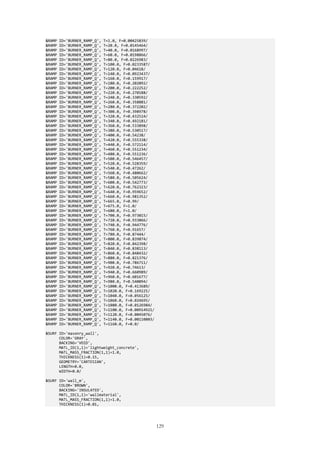
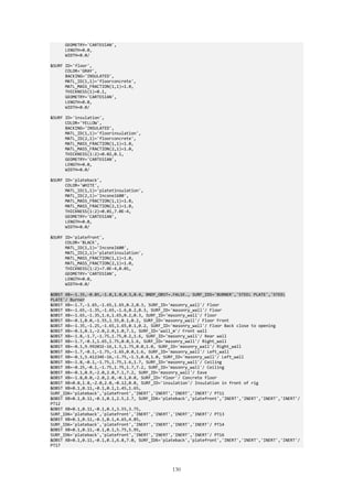
![131
&OBST XB=-1.8,-0.25,-1.75,1.75,1.7,7.2, COLOR='INVISIBLE', SURF_ID='INERT'/ Obstruction
&OBST XB=-1.8,-0.1,1.75,2.0,1.7,7.2, COLOR='INVISIBLE', SURF_ID='INERT'/ Obstruction
&OBST XB=-1.8,-0.1,-2.0,-1.75,1.7,7.2, COLOR='INVISIBLE', SURF_ID='INERT'/ Obstruction
&OBST XB=-1.35,-0.1,-1.65,-1.55,0.2,0.3, SURF_ID='masonry_wall'/ Obstruction
&OBST XB=-1.35,-0.1,1.55,1.65,0.2,0.3, SURF_ID='masonry_wall'/ Obstruction
&OBST XB=-1.35,9.85323E-16,-1.55,1.55,0.2,0.3, SURF_ID='masonry_wall'/ Obstruction
&VENT SURF_ID='OPEN', XB=1.8,1.8,-2.0,2.0,0.0,7.2/ Mesh Vent: Fire mesh [XMAX]
&VENT SURF_ID='OPEN', XB=-1.8,-1.8,-2.0,2.0,0.0,7.2/ Mesh Vent: Fire mesh [XMIN]
&VENT SURF_ID='OPEN', XB=-1.8,1.8,2.0,2.0,0.0,7.2/ Mesh Vent: Fire mesh [YMAX]
&VENT SURF_ID='OPEN', XB=-1.8,1.8,-2.0,-2.0,0.0,7.2/ Mesh Vent: Fire mesh [YMIN]
&VENT SURF_ID='OPEN', XB=-1.8,1.8,-2.0,2.0,7.2,7.2/ Mesh Vent: Fire mesh [ZMAX]
&BNDF QUANTITY='ADIABATIC SURFACE TEMPERATURE'/
&BNDF QUANTITY='NET HEAT FLUX'/
&BNDF QUANTITY='INCIDENT HEAT FLUX'/
&BNDF QUANTITY='RADIATIVE HEAT FLUX'/
&BNDF QUANTITY='WALL TEMPERATURE'/
&ISOF QUANTITY='TEMPERATURE', VALUE=300.0/
&SLCF QUANTITY='VELOCITY', VECTOR=.TRUE., PBY=0.0/
&SLCF QUANTITY='VELOCITY', VECTOR=.TRUE., PBY=0.7/
&SLCF QUANTITY='VELOCITY', VECTOR=.TRUE., PBY=-0.7/
&SLCF QUANTITY='MIXTURE FRACTION', VECTOR=.TRUE., PBY=0.0/
&SLCF QUANTITY='MIXTURE FRACTION', VECTOR=.TRUE., PBY=0.7/
&SLCF QUANTITY='MIXTURE FRACTION', VECTOR=.TRUE., PBY=-0.7/
&SLCF QUANTITY='MIXTURE FRACTION', VECTOR=.TRUE., PBX=0.2/
&SLCF QUANTITY='MIXTURE FRACTION', VECTOR=.TRUE., PBX=0.4/
&SLCF QUANTITY='MIXTURE FRACTION', VECTOR=.TRUE., PBX=0.6/
&SLCF QUANTITY='MIXTURE FRACTION', PBX=1.0/
&SLCF QUANTITY='TEMPERATURE', VECTOR=.TRUE., PBY=0.0/
&SLCF QUANTITY='TEMPERATURE', VECTOR=.TRUE., PBY=0.7/
&SLCF QUANTITY='TEMPERATURE', VECTOR=.TRUE., PBY=-0.7/
&SLCF QUANTITY='TEMPERATURE', VECTOR=.TRUE., PBX=0.1/
&SLCF QUANTITY='TEMPERATURE', VECTOR=.TRUE., PBX=0.2/
&SLCF QUANTITY='TEMPERATURE', VECTOR=.TRUE., PBX=0.4/
&SLCF QUANTITY='TEMPERATURE', VECTOR=.TRUE., PBX=0.6/
&SLCF QUANTITY='TEMPERATURE', VECTOR=.TRUE., PBX=1.0/
&SLCF QUANTITY='TURBULENCE RESOLUTION', PBY=0.0/
&SLCF QUANTITY='TURBULENCE RESOLUTION', PBX=0.6/
&SLCF QUANTITY='TURBULENCE RESOLUTION', PBX=0.2/
&SLCF QUANTITY='TURBULENCE RESOLUTION', PBX=0.4/
&SLCF QUANTITY='VELOCITY', VECTOR=.TRUE., PBX=0.15/
&SLCF QUANTITY='TEMPERATURE', VECTOR=.TRUE., PBX=0.15/
&DEVC ID='[Extra Species: oxygen] Volume Fraction above fire_MEAN', QUANTITY='VOLUME FRACTION',
SPEC_ID='OXYGEN', STATISTICS='MEAN', XB=-1.35,-1.05,-0.15,0.15,1.3,1.6/
&DEVC ID='[Extra Species: oxygen] Volume Fraction door_MEAN', QUANTITY='VOLUME FRACTION',
SPEC_ID='OXYGEN', STATISTICS='MEAN', XB=-0.1,0.0,-1.5,1.5,0.3,1.0/
&TAIL /](https://image.slidesharecdn.com/b9c25bc4-7009-433b-9915-9df65ba0719b-160222143636/85/Report_5510_Markus_Nilsson-143-320.jpg)
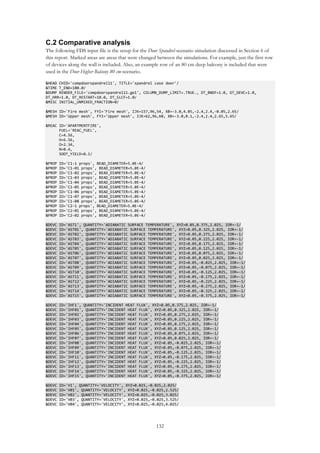

![134
MATL_MASS_FRACTION(1,1)=1.0,
THICKNESS(1)=0.1,
GEOMETRY='CARTESIAN',
LENGTH=0.0,
WIDTH=0.0/
&SURF ID='WALL',
RGB=255,255,102,
BACKING='VOID',
MATL_ID(1,1)='CONCRETE',
MATL_MASS_FRACTION(1,1)=1.0,
THICKNESS(1)=0.1,
GEOMETRY='CARTESIAN',
LENGTH=0.0,
WIDTH=0.0/
&SURF ID='FIRE',
COLOR='RED',
HRRPUA=3100.0,
RAMP_Q='FIRE_RAMP_Q'/
&RAMP ID='FIRE_RAMP_Q', T=0.0, F=0.0/
&RAMP ID='FIRE_RAMP_Q', T=10.0, F=1.0/
&RAMP ID='FIRE_RAMP_Q', T=180.0, F=1.0/
&OBST XB=0.05,0.1,-0.4,0.4,2.55,3.2, SURF_ID='FACADE WALL'/ Spandrel
&OBST XB=0.05,0.1,-0.4,0.4,3.2,5.2, SURF_ID='Window'/ Door up
&OBST XB=0.05,0.1,0.4,2.3,2.55,5.6, SURF_ID='FACADE WALL'/ WallUp
&OBST XB=0.05,0.1,-0.4,0.4,5.2,5.6, SURF_ID='FACADE WALL'/ WallUp
&OBST XB=0.05,0.1,-2.3,-0.4,2.55,5.6, SURF_ID='FACADE WALL'/ WallUp
&OBST XB=0.05,0.1,-2.3,2.3,0.0,2.5, SURF_ID='FRONT WALL'/ WallDown
&OBST XB=0.1,4.6,2.25,2.3,0.0,2.5, COLOR='INVISIBLE', SURF_ID='WALL'/ WallDown
&OBST XB=0.1,4.6,-2.3,-2.25,0.0,2.5, SURF_ID='WALL'/ WallDown
&OBST XB=4.6,4.65,-2.3,2.3,0.0,2.5, SURF_ID='WALL'/ WallDown
&OBST XB=0.05,4.65,-2.3,2.3,-0.05,0.0, COLOR='GRAY 40', SURF_ID='WALL'/ FloorGround
&OBST XB=0.05,4.65,-2.3,2.3,2.5,2.55, COLOR='GRAY 40', SURF_ID='WALL'/ FloorBetween
&OBST XB=1.85,2.85,-0.5,0.5,0.0,0.2, COLOR='RED', BNDF_OBST=.FALSE., SURF_IDS='FIRE','INERT','INERT'/
Burner
&OBST XB=0.05,0.1,-2.3,2.3,5.6,5.65, COLOR='GRAY 40', SURF_ID='FACADE WALL'/ FloorBetween
&OBST XB=0.1,4.65,-2.4,2.4,2.55,2.65, COLOR='INVISIBLE', SURF_ID='INERT'/ Inert Obstruction
&OBST XB=-0.75,0.05,-0.8,0.8,2.35,2.55, COLOR='GRAY 20', SURF_ID='FACADE WALL'/ Balcony 80 cm
&HOLE XB=4.6,4.65,-2.0,2.0,0.0,0.4/ Hole
&HOLE XB=0.05,0.1,-0.4,0.4,0.0,2.0/ DoorDown
&VENT SURF_ID='OPEN', XB=4.85,4.85,-2.4,2.4,-0.05,2.65/ Mesh Vent: Fire mesh [XMAX]
&VENT SURF_ID='OPEN', XB=-3.0,-3.0,-2.4,2.4,-0.05,2.65/ Mesh Vent: Fire mesh [XMIN]
&VENT SURF_ID='OPEN', XB=-3.0,4.85,2.4,2.4,-0.05,2.65/ Mesh Vent: Fire mesh [YMAX]
&VENT SURF_ID='OPEN', XB=-3.0,4.85,-2.4,-2.4,-0.05,2.65/ Mesh Vent: Fire mesh [YMIN]
&VENT SURF_ID='OPEN', XB=0.1,4.85,-2.4,2.4,2.65,2.65/ Mesh Vent: Fire mesh [ZMAX]
&VENT SURF_ID='OPEN', XB=-3.0,4.85,-2.4,2.4,-0.05,-0.05/ Mesh Vent: Fire mesh [ZMIN]
&VENT SURF_ID='OPEN', XB=0.1,0.1,-2.4,2.4,2.65,5.65/ Mesh Vent: Upper mesh [XMAX]
&VENT SURF_ID='OPEN', XB=-3.0,-3.0,-2.4,2.4,2.65,5.65/ Mesh Vent: Upper mesh [XMIN]
&VENT SURF_ID='OPEN', XB=-3.0,0.1,2.4,2.4,2.65,5.65/ Mesh Vent: Upper mesh [YMAX]
&VENT SURF_ID='OPEN', XB=-3.0,0.1,-2.4,-2.4,2.65,5.65/ Mesh Vent: Upper mesh [YMIN]
&VENT SURF_ID='OPEN', XB=-3.0,0.1,-2.4,2.4,5.65,5.65/ Mesh Vent: Upper mesh [ZMAX]
&BNDF QUANTITY='ADIABATIC SURFACE TEMPERATURE'/
&BNDF QUANTITY='CONVECTIVE HEAT FLUX'/
&BNDF QUANTITY='GAUGE HEAT FLUX'/
&BNDF QUANTITY='NET HEAT FLUX'/
&BNDF QUANTITY='INCIDENT HEAT FLUX'/
&BNDF QUANTITY='RADIATIVE HEAT FLUX'/
&BNDF QUANTITY='RADIOMETER'/
&BNDF QUANTITY='WALL TEMPERATURE'/
&ISOF QUANTITY='TEMPERATURE', VALUE=300.0/
&SLCF QUANTITY='PRESSURE', PBY=0.0/
&SLCF QUANTITY='MIXTURE FRACTION', VECTOR=.TRUE., PBX=-0.05/
&SLCF QUANTITY='MIXTURE FRACTION', VECTOR=.TRUE., PBX=-0.1/
&SLCF QUANTITY='MIXTURE FRACTION', VECTOR=.TRUE., PBX=-0.2/
&SLCF QUANTITY='MIXTURE FRACTION', VECTOR=.TRUE., PBX=-0.4/
&SLCF QUANTITY='MIXTURE FRACTION', VECTOR=.TRUE., PBX=-0.6/
&SLCF QUANTITY='MIXTURE FRACTION', VECTOR=.TRUE., PBX=-0.8/
&SLCF QUANTITY='MIXTURE FRACTION', VECTOR=.TRUE., PBX=-1.0/
&SLCF QUANTITY='MIXTURE FRACTION', VECTOR=.TRUE., PBX=-1.2/
&SLCF QUANTITY='MIXTURE FRACTION', VECTOR=.TRUE., PBX=-1.4/
&SLCF QUANTITY='MIXTURE FRACTION', VECTOR=.TRUE., PBX=-1.6/](https://image.slidesharecdn.com/b9c25bc4-7009-433b-9915-9df65ba0719b-160222143636/85/Report_5510_Markus_Nilsson-146-320.jpg)
![135
&SLCF QUANTITY='MIXTURE FRACTION', VECTOR=.TRUE., PBY=0.0/
&SLCF QUANTITY='TURBULENCE RESOLUTION', PBY=0.0/
&SLCF QUANTITY='TURBULENCE RESOLUTION', PBX=-0.1/
&SLCF QUANTITY='VELOCITY', VECTOR=.TRUE., PBY=0.0/
&SLCF QUANTITY='VELOCITY', VECTOR=.TRUE., PBZ=0.2/
&SLCF QUANTITY='VELOCITY', VECTOR=.TRUE., PBX=-0.05/
&SLCF QUANTITY='TEMPERATURE', VECTOR=.TRUE., PBY=0.0/
&SLCF QUANTITY='TEMPERATURE', VECTOR=.TRUE., PBY=1.1/
&SLCF QUANTITY='TEMPERATURE', VECTOR=.TRUE., PBY=-1.1/
&SLCF QUANTITY='TEMPERATURE', VECTOR=.TRUE., PBX=0.0/
&SLCF QUANTITY='TEMPERATURE', VECTOR=.TRUE., PBX=-0.05/
&SLCF QUANTITY='TEMPERATURE', VECTOR=.TRUE., PBX=-0.1/
&SLCF QUANTITY='TEMPERATURE', VECTOR=.TRUE., PBX=-0.2/
&SLCF QUANTITY='TEMPERATURE', VECTOR=.TRUE., PBX=-0.4/
&SLCF QUANTITY='TEMPERATURE', VECTOR=.TRUE., PBX=-0.5/
&SLCF QUANTITY='TEMPERATURE', VECTOR=.TRUE., PBX=-0.6/
&SLCF QUANTITY='TEMPERATURE', VECTOR=.TRUE., PBX=-0.8/
&SLCF QUANTITY='TEMPERATURE', VECTOR=.TRUE., PBX=-1.0/
&SLCF QUANTITY='TEMPERATURE', VECTOR=.TRUE., PBX=-1.2/
&SLCF QUANTITY='TEMPERATURE', VECTOR=.TRUE., PBX=-1.4/
&SLCF QUANTITY='TEMPERATURE', VECTOR=.TRUE., PBX=-1.6/
&DEVC ID='[Extra Species: oxygen] Volume Fraction_MEAN', QUANTITY='VOLUME FRACTION', SPEC_ID='OXYGEN',
STATISTICS='MEAN', XB=0.1,0.4,-2.25,-1.95,0.0,0.3/
&DEVC ID='[Extra Species: oxygen] Volume Fraction door_MEAN', QUANTITY='VOLUME FRACTION',
SPEC_ID='OXYGEN', STATISTICS='MEAN', XB=0.05,0.1,-0.4,0.4,0.0,2.0/
&DEVC ID='[Extra Species: oxygen] Volume Fraction abbove fire_MEAN', QUANTITY='VOLUME FRACTION',
SPEC_ID='OXYGEN', STATISTICS='MEAN', XB=2.2,2.5,-0.15,0.15,2.2,2.5/
&DEVC ID='Gas Temperature door_MEAN', QUANTITY='GAS TEMPERATURE', STATISTICS='MEAN', XB=0.0,0.1,-
0.4,0.4,0.0,2.0/
&DEVC ID='Gas Temperature door_MAX', QUANTITY='GAS TEMPERATURE', STATISTICS='MAX', XB=0.0,0.1,-
0.4,0.4,0.0,2.0/
&DEVC ID='Glass temperature_MEAN', QUANTITY='WALL TEMPERATURE', STATISTICS='MEAN', XB=0.05,0.1,-
0.4,0.4,3.2,5.2/
&DEVC ID='Glass temperature_MIN', QUANTITY='WALL TEMPERATURE', STATISTICS='MIN', XB=0.05,0.1,-
0.4,0.4,3.2,5.2/
&DEVC ID='Glass temperature_MAX', QUANTITY='WALL TEMPERATURE', STATISTICS='MAX', XB=0.05,0.1,-
0.4,0.4,3.2,5.2/
&TAIL /.](https://image.slidesharecdn.com/b9c25bc4-7009-433b-9915-9df65ba0719b-160222143636/85/Report_5510_Markus_Nilsson-147-320.jpg)


