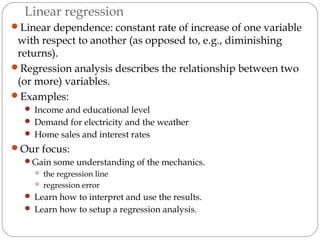
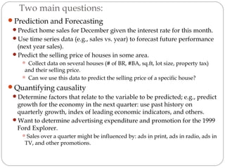
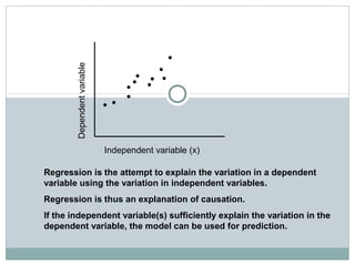
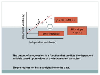
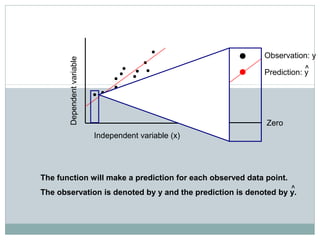
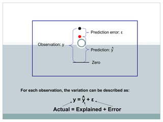
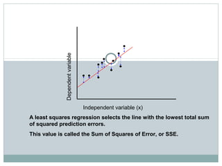
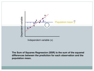
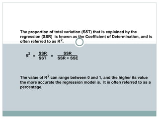
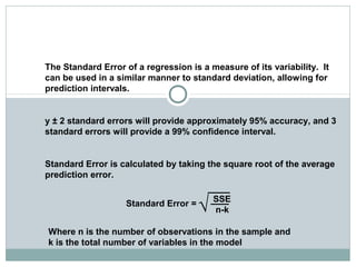
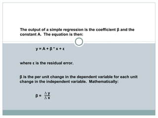
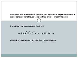
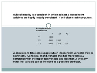
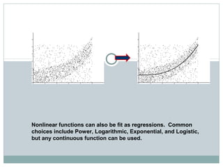
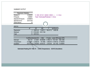
Regression analysis is used to identify relationships between variables and make predictions. Simple linear regression fits a straight line to data using one independent variable to predict a dependent variable. Multiple linear regression uses more than one independent variable to explain variance in the dependent variable. The goal is to select variables that sufficiently explain variation in the dependent variable to allow for accurate prediction. Key outputs of regression include coefficients, R-squared, standard error, and significance values.

1. Regression Analysis
BY- RIA KACHHAWAHA
IBS GURGAON

2. Regression: Introduction
BASIC IDEA:
USE DATA TO IDENTIFY RELATIONSHIPS AMONG
VARIABLES AND USE THESE RELATIONSHIPS TO MAKE
PREDICTIONS.

3. Linear regression
Linear dependence: constant rate of increase of one variable
with respect to another (as opposed to, e.g., diminishing
returns).
Regression analysis describes the relationship between two
(or more) variables.
Examples:
 Income and educational level
 Demand for electricity and the weather
 Home sales and interest rates
Our focus:
Gain some understanding of the mechanics.
 the regression line
 regression error
 Learn how to interpret and use the results.
 Learn how to setup a regression analysis.

4. Two main questions:
Prediction and Forecasting
Predict home sales for December given the interest rate for this month.
Use time series data (e.g., sales vs. year) to forecast future performance
(next year sales).
Predict the selling price of houses in some area.
 Collect data on several houses (# of BR, #BA, sq.ft, lot size, property tax)
and their selling price.
 Can we use this data to predict the selling price of a specific house?
Quantifying causality
Determine factors that relate to the variable to be predicted; e.g., predict
growth for the economy in the next quarter: use past history on
quarterly growth, index of leading economic indicators, and others.
Want to determine advertising expenditure and promotion for the 1999
Ford Explorer.
Sales over a quarter might be influenced by: ads in print, ads in radio, ads in
TV, and other promotions.

5. Regression
Regression is the attempt to explain the variation in a dependent
variable using the variation in independent variables.
Regression is thus an explanation of causation.
If the independent variable(s) sufficiently explain the variation in the
dependent variable, the model can be used for prediction.
Independent variable (x)
Dependentvariable

6. Simple Linear Regression
Independent variable (x)
Dependentvariable(y)
The output of a regression is a function that predicts the dependent
variable based upon values of the independent variables.
Simple regression fits a straight line to the data.
y’ = b0 + b1X ± є
b0 (y intercept)
B1 = slope
= ∆y/ ∆x
є

7. Simple Linear Regression
Independent variable (x)
Dependentvariable
The function will make a prediction for each observed data point.
The observation is denoted by y and the prediction is denoted by y.
Zero
Prediction: y
Observation: y
^
^

8. Simple Linear Regression
For each observation, the variation can be described as:
y = y + ε
Actual = Explained + Error
Zero
Prediction error: ε
^
Prediction: y^
Observation: y

9. Regression
Independent variable (x)
Dependentvariable
A least squares regression selects the line with the lowest total sum
of squared prediction errors.
This value is called the Sum of Squares of Error, or SSE.

10. Calculating SSR
Independent variable (x)
Dependentvariable
The Sum of Squares Regression (SSR) is the sum of the squared
differences between the prediction for each observation and the
population mean.
Population mean: y

11. Regression Formulas
The Total Sum of Squares (SST) is equal to SSR + SSE.
Mathematically,
SSR = ∑ ( y – y ) (measure of explained variation)
SSE = ∑ ( y – y ) (measure of unexplained variation)
SST = SSR + SSE = ∑ ( y – y ) (measure of total variation in y)
^
^
2
2

12. The Coefficient of Determination
The proportion of total variation (SST) that is explained by the
regression (SSR) is known as the Coefficient of Determination, and is
often referred to as R .
R = =
The value of R can range between 0 and 1, and the higher its value
the more accurate the regression model is. It is often referred to as a
percentage.
SSR SSR
SST SSR + SSE
2
2
2

13. Standard Error of Regression
The Standard Error of a regression is a measure of its variability. It
can be used in a similar manner to standard deviation, allowing for
prediction intervals.
y ± 2 standard errors will provide approximately 95% accuracy, and 3
standard errors will provide a 99% confidence interval.
Standard Error is calculated by taking the square root of the average
prediction error.
Standard Error =
SSE
n-k
Where n is the number of observations in the sample and
k is the total number of variables in the model
√

14. The output of a simple regression is the coefficient β and the
constant A. The equation is then:
y = A + β * x + ε
where ε is the residual error.
β is the per unit change in the dependent variable for each unit
change in the independent variable. Mathematically:
β =
∆ y
∆ x

15. Multiple Linear Regression
More than one independent variable can be used to explain variance in
the dependent variable, as long as they are not linearly related.
A multiple regression takes the form:
y = A + β X + β X + … + β k Xk + ε
where k is the number of variables, or parameters.
1 1 2 2

16. Multicollinearity
Multicollinearity is a condition in which at least 2 independent
variables are highly linearly correlated. It will often crash computers.
Example table of
Correlations
Y X1 X2
Y 1.000
X1 0.802 1.000
X2 0.848 0.578 1.000
A correlations table can suggest which independent variables may be
significant. Generally, an ind. variable that has more than a .3
correlation with the dependent variable and less than .7 with any
other ind. variable can be included as a possible predictor.

17. Nonlinear Regression
Nonlinear functions can also be fit as regressions. Common
choices include Power, Logarithmic, Exponential, and Logistic,
but any continuous function can be used.

18. Regression Output in Excel
SUMMARY OUTPUT
Regression Statistics
Multiple R 0.982655
R Square 0.96561
Adjusted R Square 0.959879
Standard Error 26.01378
Observations 15
ANOVA
df SS MS F Significance F
Regression 2 228014.6 114007.3 168.4712 1.65E-09
Residual 12 8120.603 676.7169
Total 14 236135.2
CoefficientsStandard Error t Stat P-value Lower 95%Upper 95%
Intercept 562.151 21.0931 26.65094 4.78E-12 516.1931 608.1089
Temperature -5.436581 0.336216 -16.1699 1.64E-09 -6.169133 -4.704029
Insulation -20.01232 2.342505 -8.543127 1.91E-06 -25.1162 -14.90844
Estimated Heating Oil = 562.15 - 5.436 (Temperature) - 20.012 (Insulation)
Y = B0 + B1 X1 + B2X2 + B3X3 - - - +/- Error
Total = Estimated/Predicted +/- Error

19. SOURCE: MARKETING RESEARCH TEXT BOOK (MALHOTRA, 1988)