This document discusses methods for estimating missing rainfall data, including simple arithmetic averaging if normal annual precipitation is within 10% between stations, and a normal ratio method if precipitation varies considerably. It also discusses consistency testing of rainfall records using a double mass curve technique to identify changes in rainfall regimes. Methods for determining mean precipitation over an area using Thiessen polygons and isohyetal mapping are presented. The relationship between rainfall intensity, duration and frequency is examined through intensity-duration-frequency and depth-duration curves. An example illustrates plotting a rainfall hyetograph and intensity-duration curve from mass curve data.

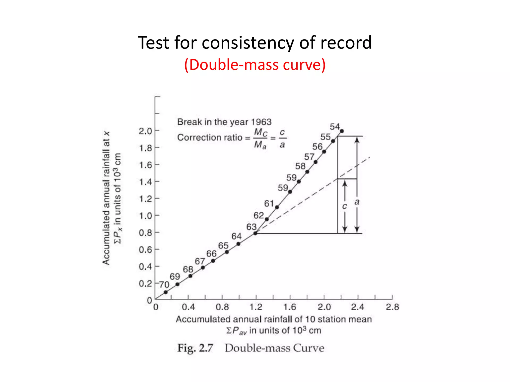
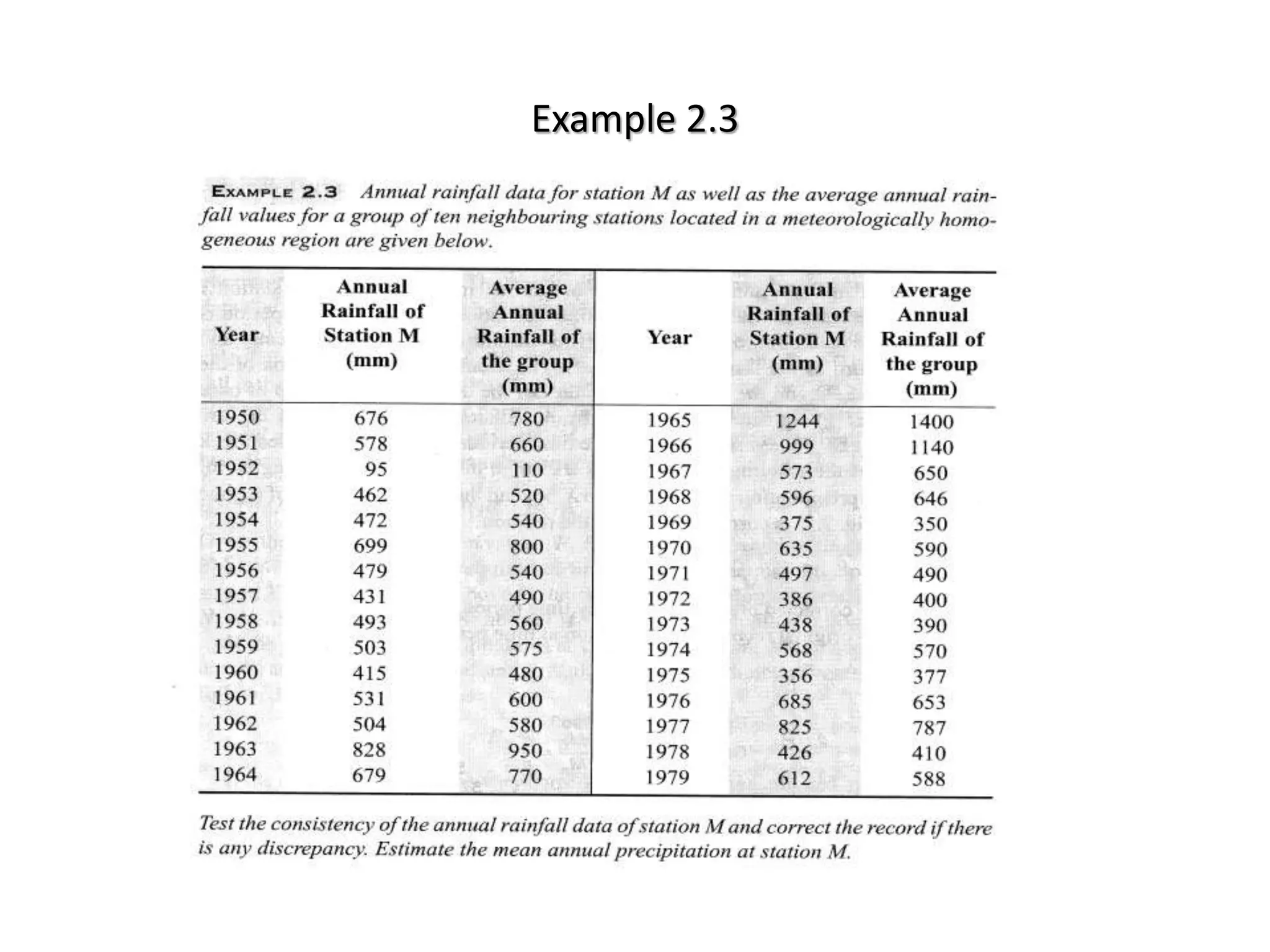
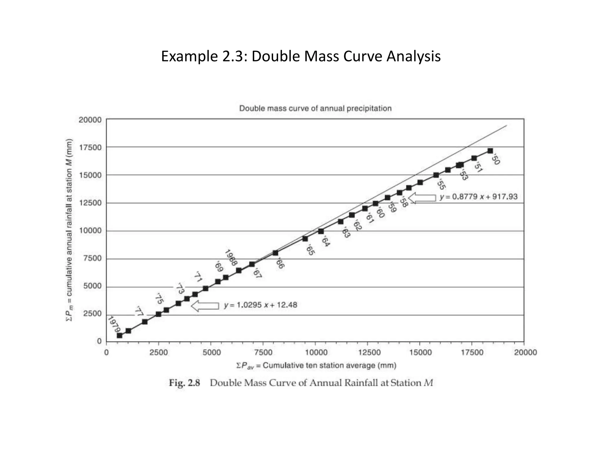
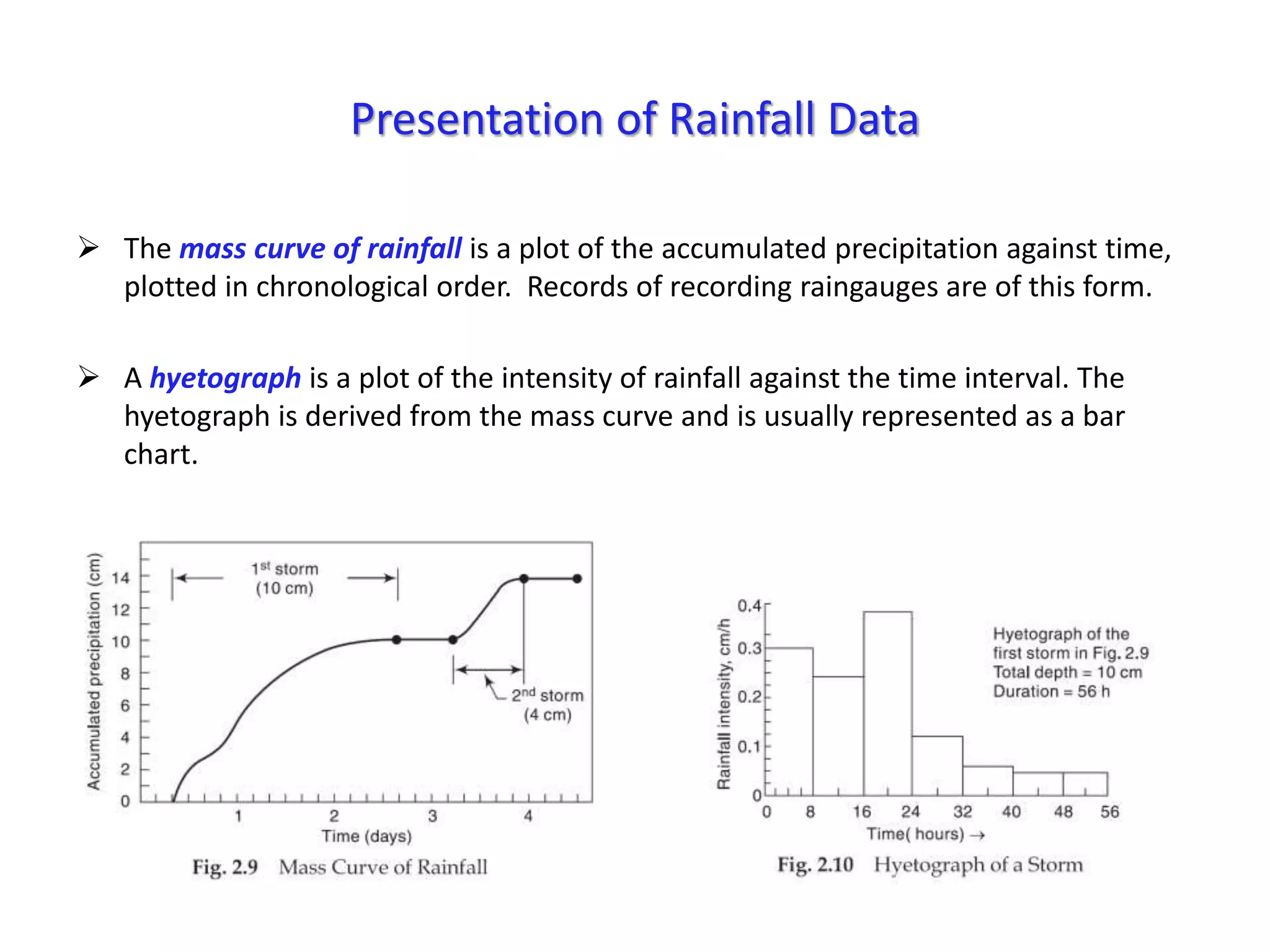
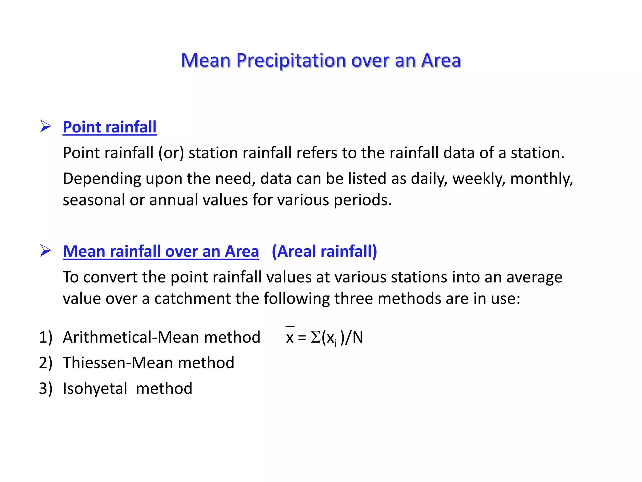
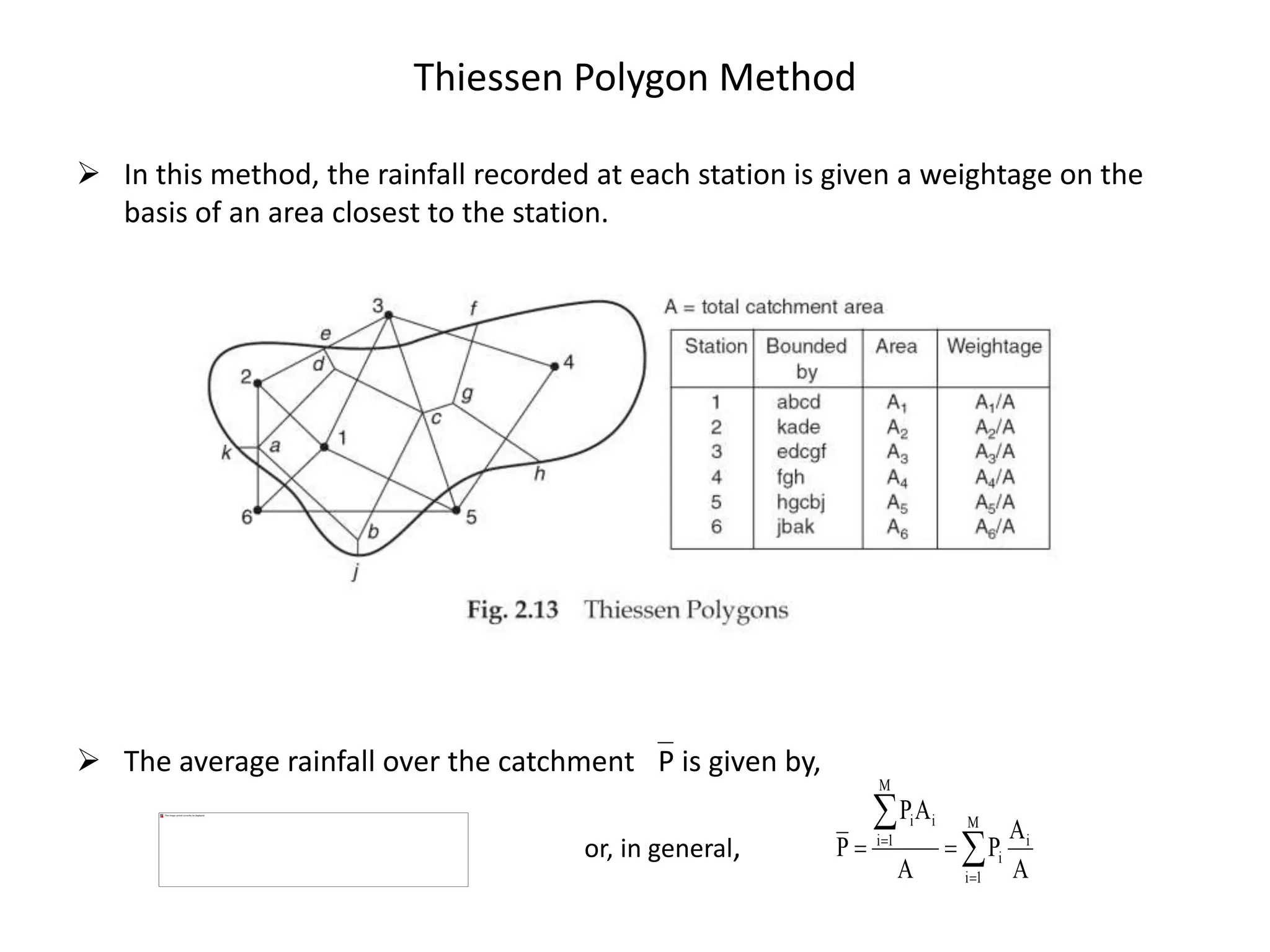
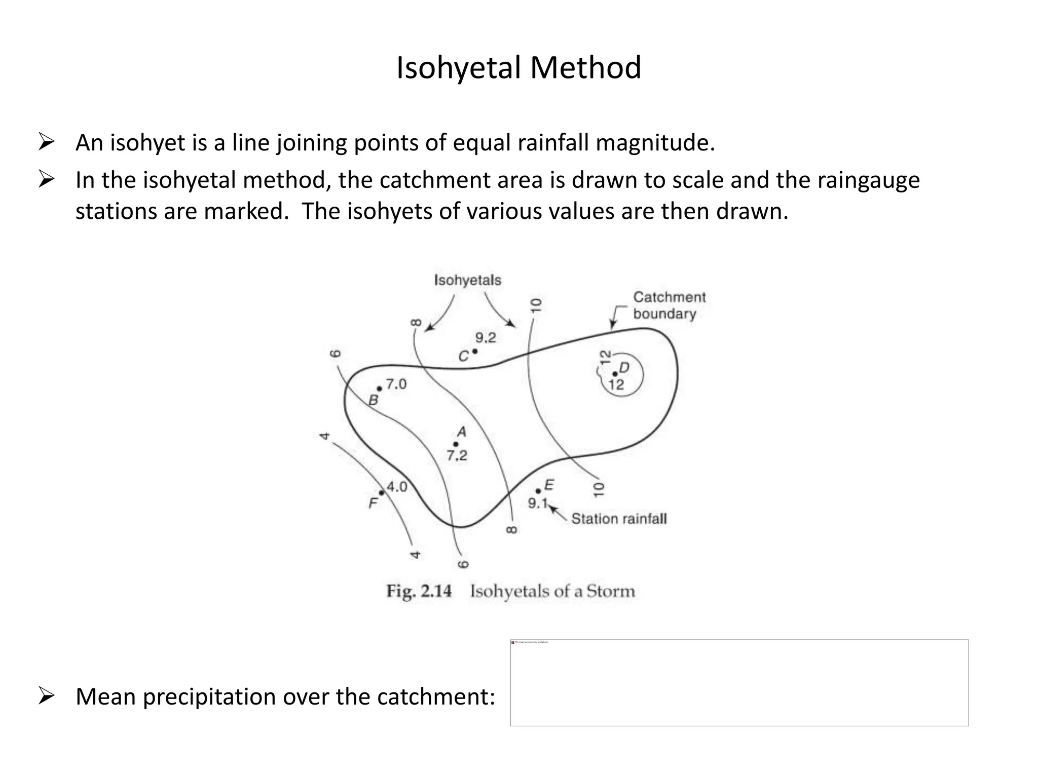
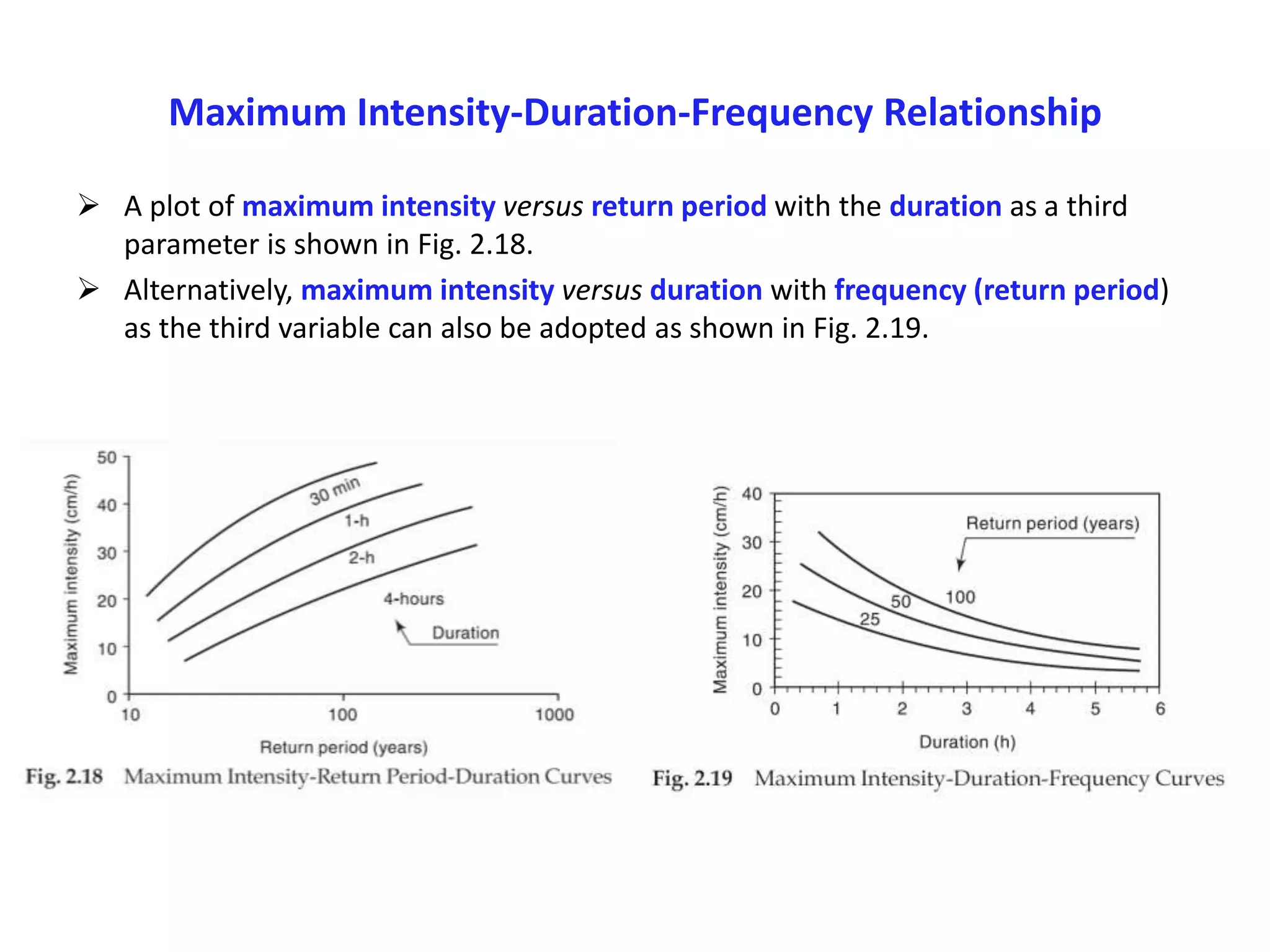
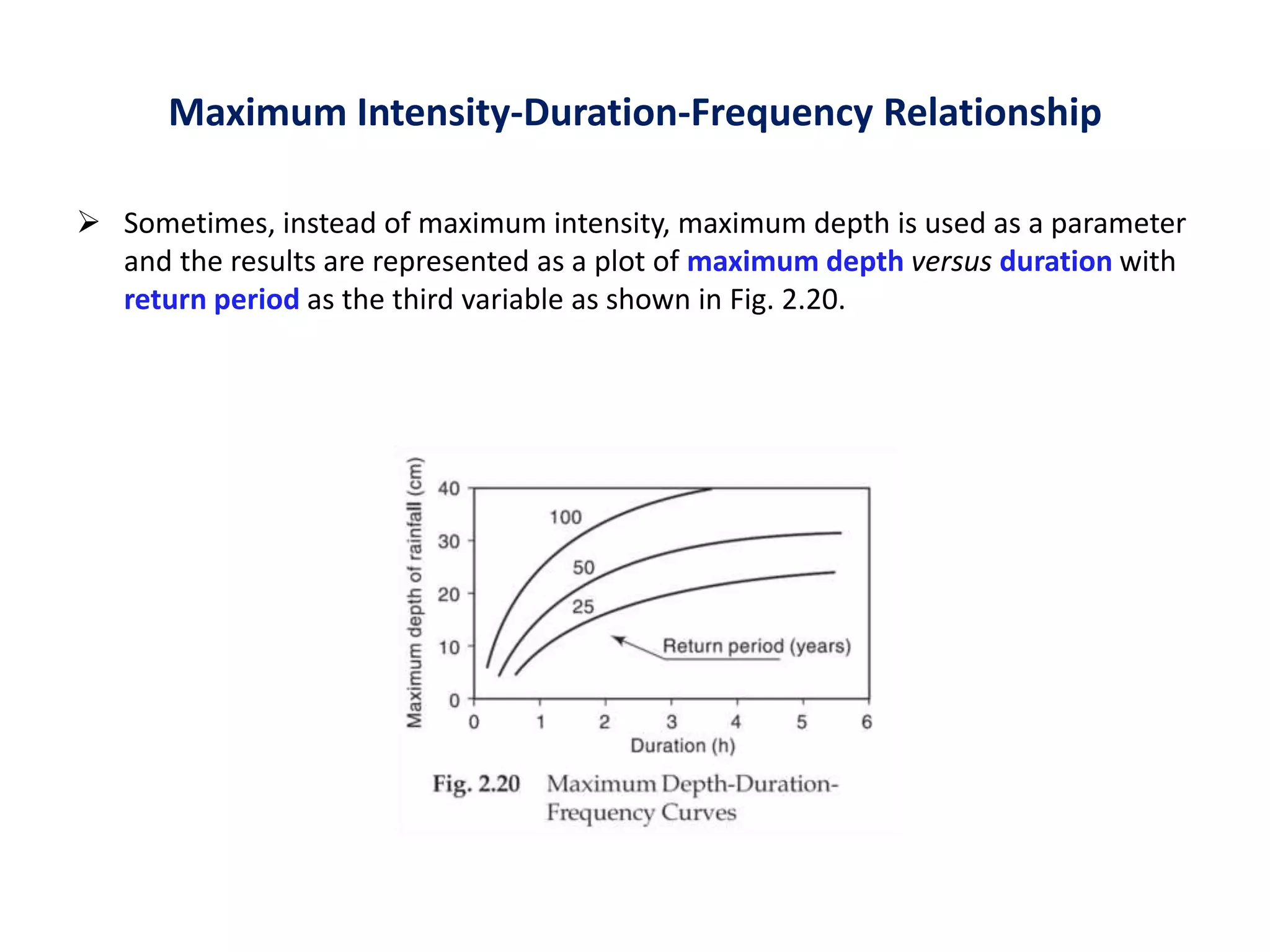
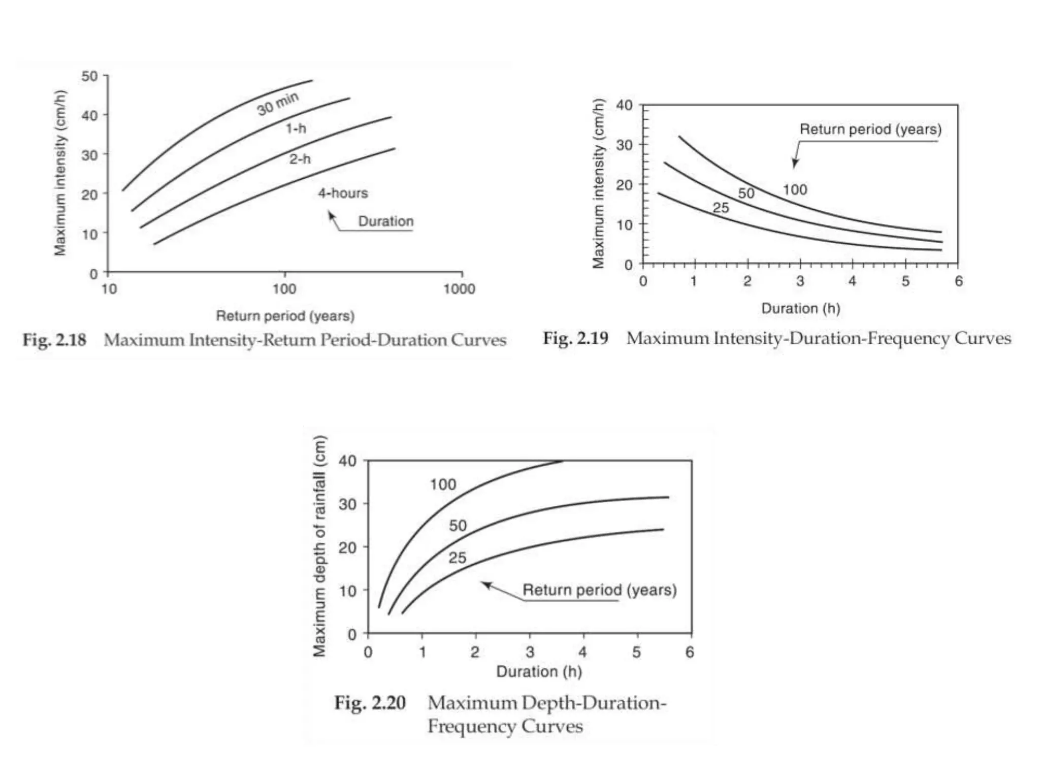
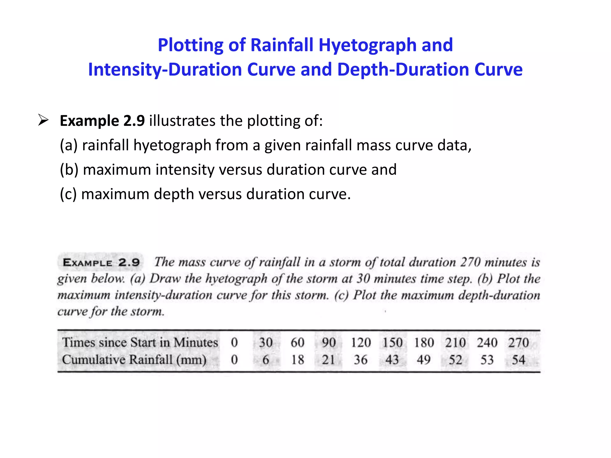
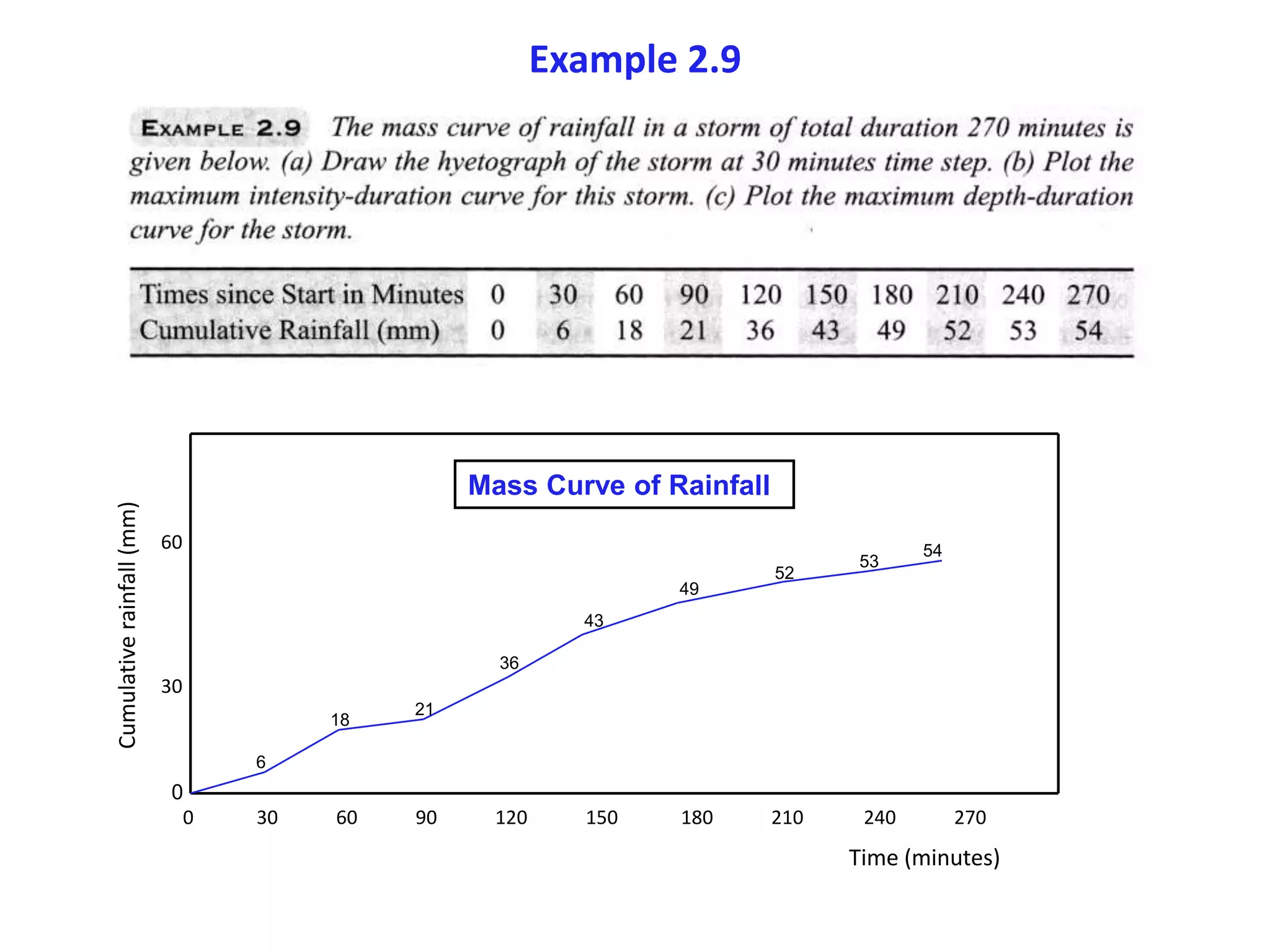
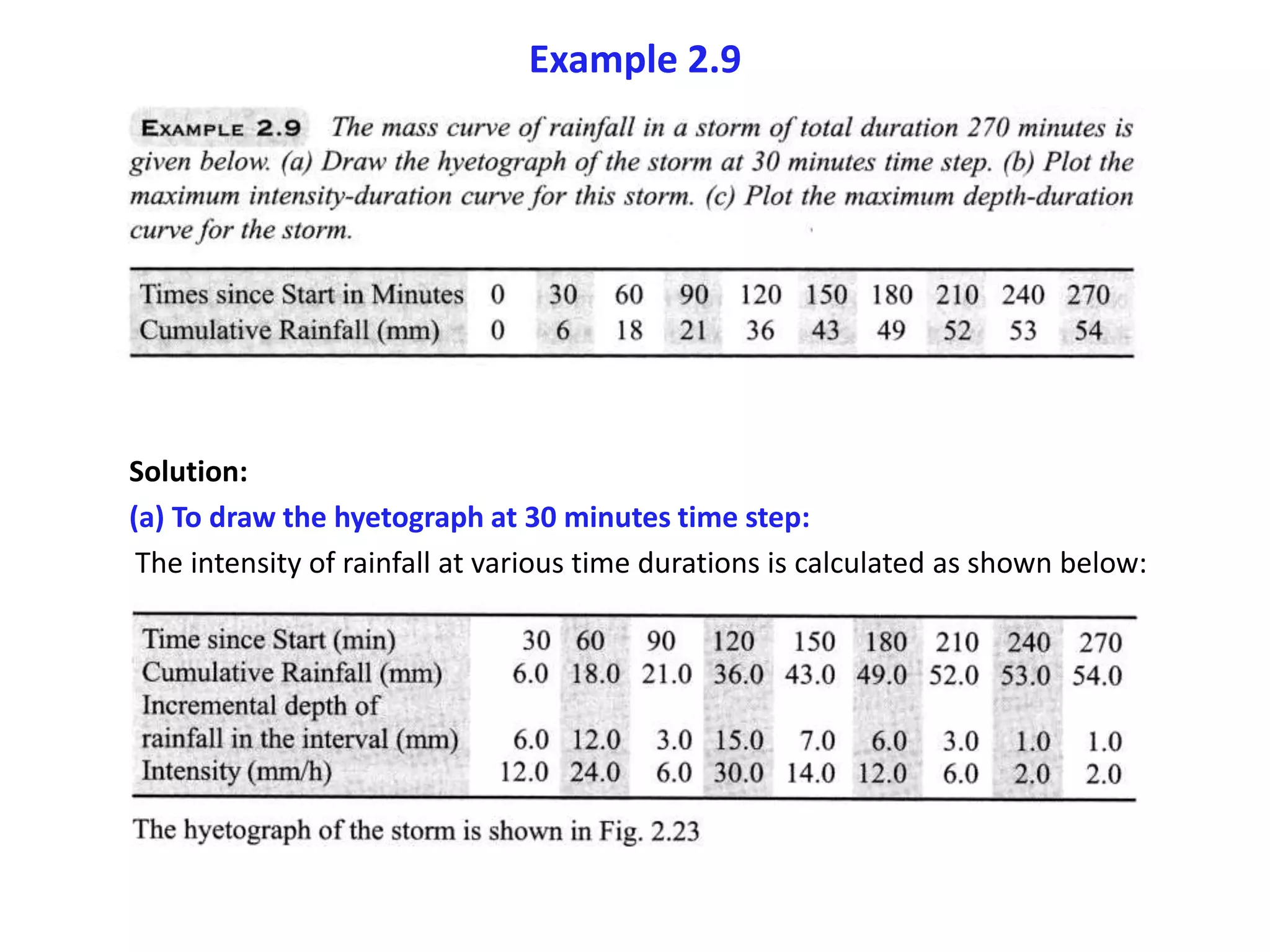
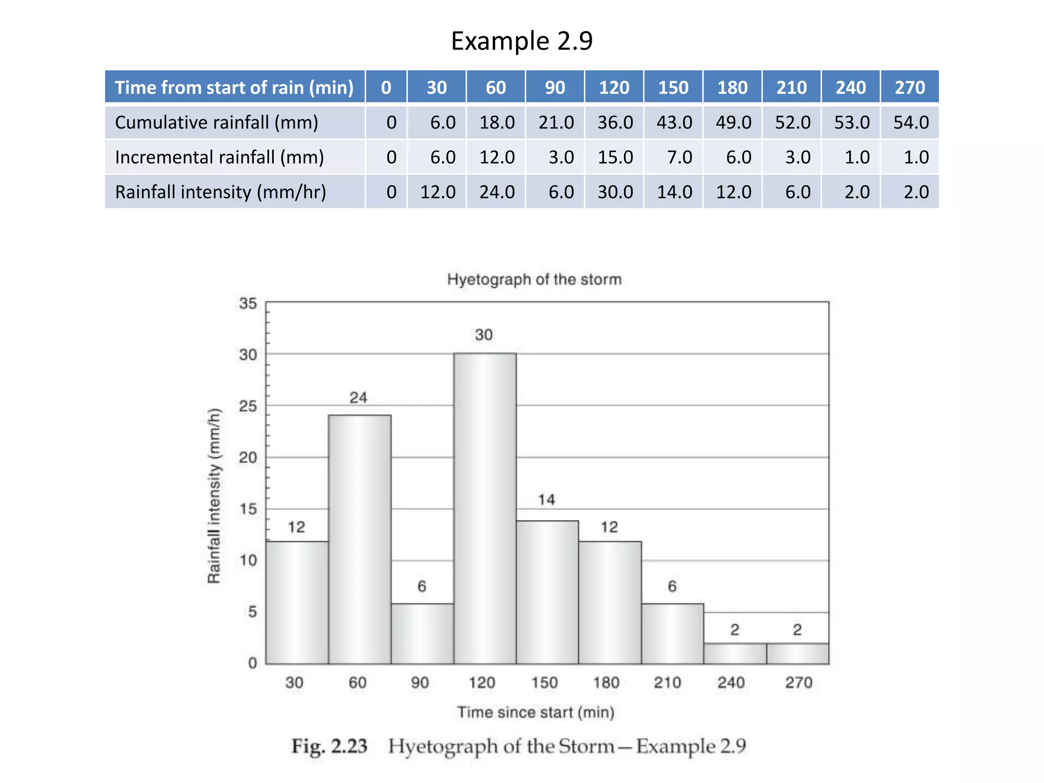
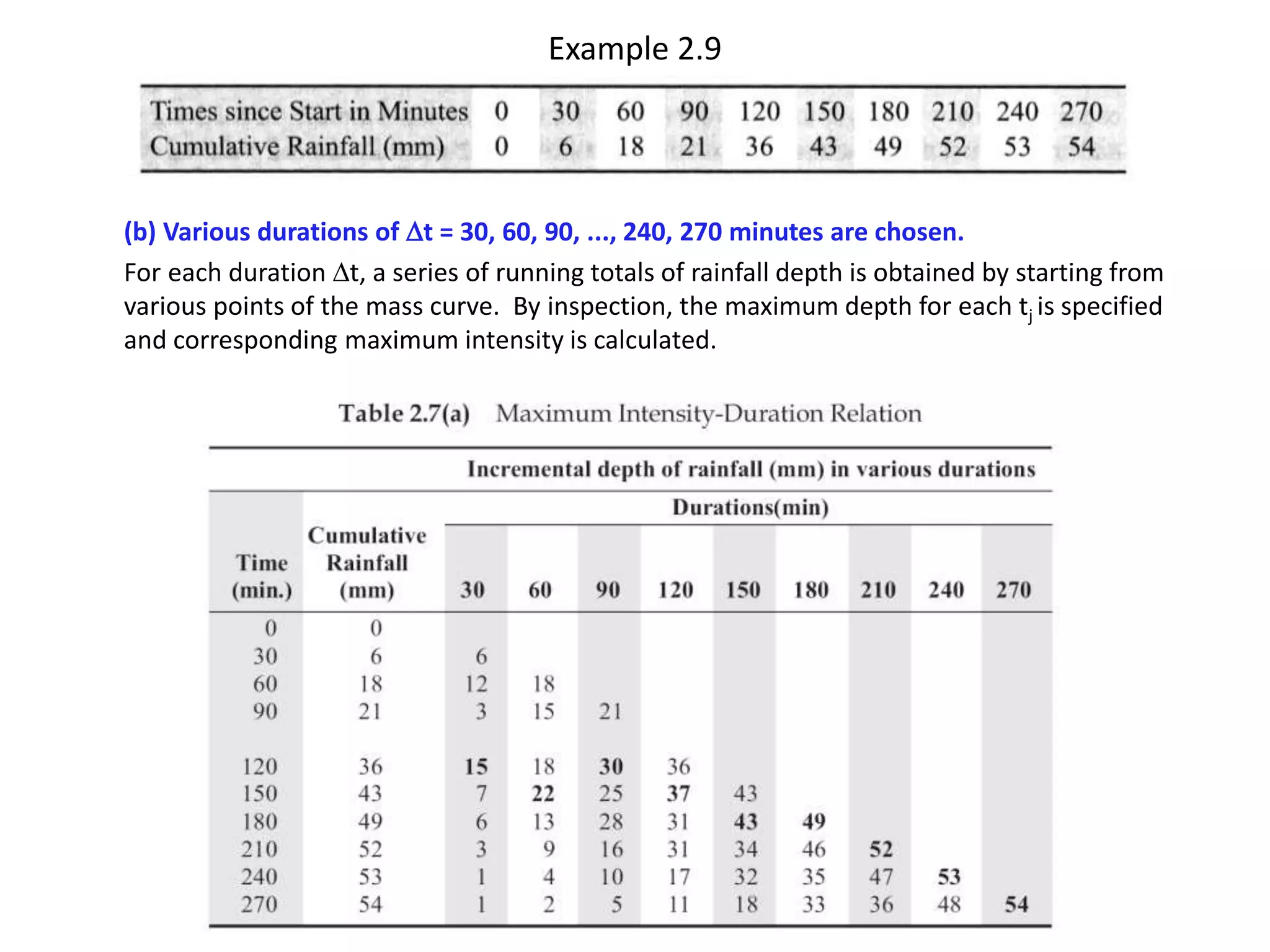
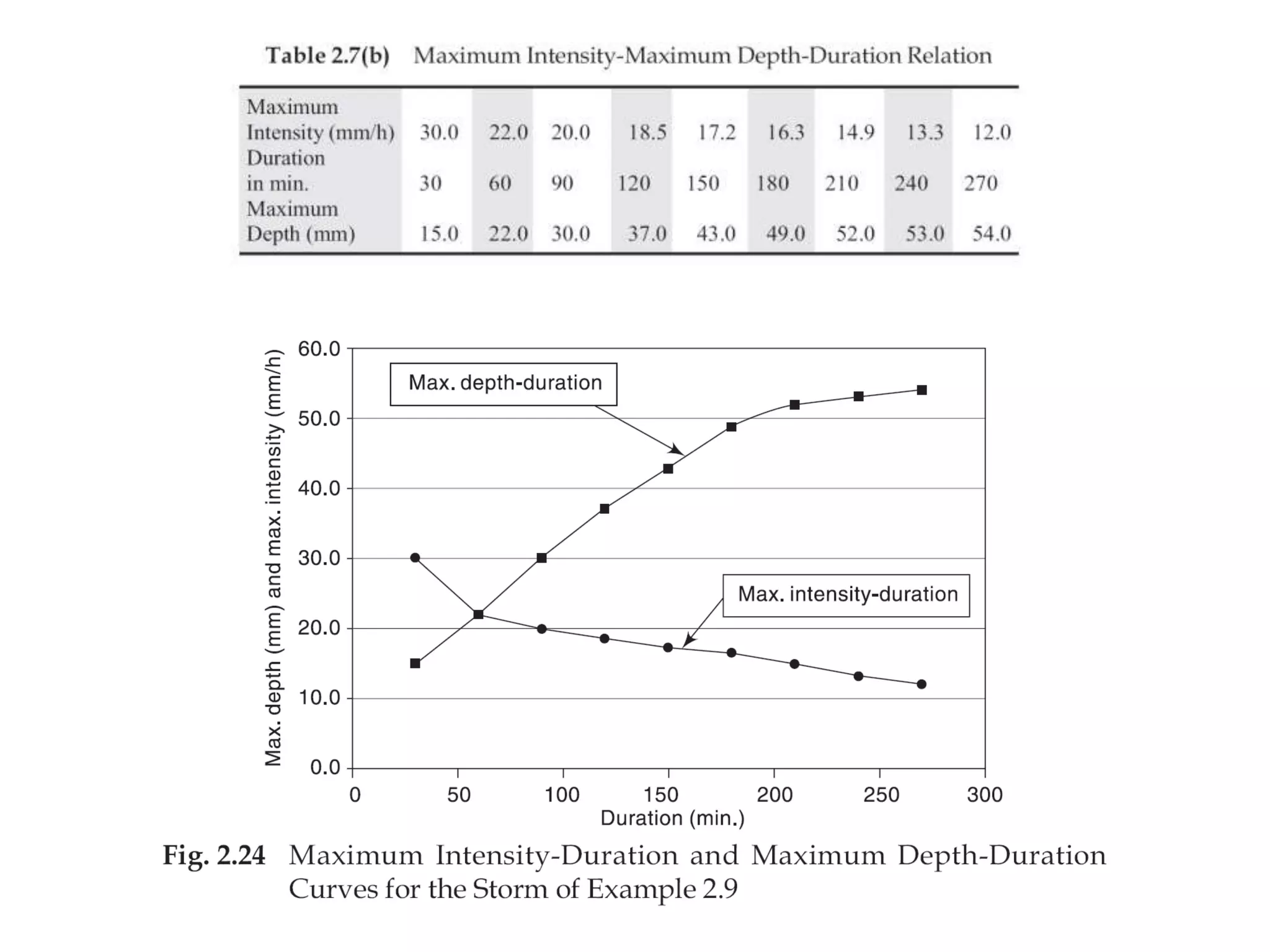
1. Precipitation Analysis (Solved
Examples)

2. Estimation of missing Rainfall Data
 Given the annual precipitation values, P1, P2, P3,….,Pm at neighbouring M stations 1, 2, 3, ….,M
respectively. It is required to find the missing annual precipitation Px at a station X not included
in the above M stations.
1. If the normal annual precipitations at various stations are within about 10% of the normal
annual precipitation at station X, then a simple arithmetic average procedure is used to
estimate Px. Thus
(2.4)
2. If the normal precipitations vary considerably, then Px is estimated by weighing the
precipitation at the various stations by the ratios of normal annual precipitations. This method,
known as the normal ratio method, gives Px as
(or)
(2.5)
]
......
[
1
2
1 m
x P
P
P
M
P 



]
........
[
1
2
2
1
1
m
m
m
x
x
x P
N
N
P
N
N
P
N
N
M
P 



]
......
[
2
2
1
1
m
m
x
x
N
P
N
P
N
P
M
N
P 




3. Example 2.2
 The normal annual rainfall at stations A, B, C, and D in a basin are 80.97, 67.59,
76.28 and 92.01 cm respectively. In the year 1975, the station D was inoperative
and the stations A, B and C recorded annual precipitations of 91.11, 72.23 and
79.89 cm respectively. Estimate the rainfall at station D in that year.
 As the normal rainfall values vary more than 10%, the normal ratio
method is adopted.
cm
48
.
99
]
28
.
76
89
.
79
59
.
67
23
.
72
79
.
80
11
.
91
[
x
3
01
.
92
PD 



]
......
[
2
2
1
1
m
m
x
x
N
P
N
P
N
P
M
N
P 




4. Test for consistency of record
 If the conditions relevant to the recording of a raingauge station have undergone a
significant change during the period of record, inconsistency would arise in the
rainfall data of that station.
 This inconsistency would be felt from the time the significant change took place.
 Some of the common causes for inconsistency of record are:
i. shifting of a raingauge station to a new location,
ii. the neighbourhood of the station undergoing a marked change,
iii. change in the ecosystem due to calamities, such as forest fires, land slides, and
iv. occurrence of observational error from a certain date.
 Checking for inconsistency of a record is done by the double–mass curve technique.
This technique is based on the principle that when each recorded data comes from
the same parent population, they are consistent.

5. Test for consistency of record
(Double-mass curve)

6. Example 2.3

7. Example 2.3
 The rainfall data is sorted in descending order of the year, starting from the latest
year 1979.
 Cumulative values of station M rainfall (Pm) and the ten station average rainfall
values (Pav) are calculated as shown in Table 2.1.
 The data is then plotted with Pm on the Y-axis and Pav on the X-axis to obtain a
double-mass curve plot.
 The year corresponding to the plotted points is also noted on the plot.
 It is seen that the data plots as two straight lines with a break of slope at the year
1969.
This represents a change in the regime of the station M after the year 1968.

8. Example 2.3
 The slope of the best straight line for the period (1979-1969) is Mc = 1.0295 and
the slope of the best straight line for the period (1968-1950) is Ma= 0.8779.
 The correction ratio to bring the old records (1950 to 1968) to the current regime
is,
Mc/ Ma = 1.0295/0.8779 = 1.173
 Each of the pre 1969 annual rainfall value is multiplied by the correction ratio of
1.173 to get the adjusted value as shown in the last column of Table 2.1.
 The mean annual precipitation at station M is 19004/30 = 633.5 mm

9. 793
∑

10. Example 2.3: Double Mass Curve Analysis

11. Presentation of Rainfall Data
 The mass curve of rainfall is a plot of the accumulated precipitation against time,
plotted in chronological order. Records of recording raingauges are of this form.
 A hyetograph is a plot of the intensity of rainfall against the time interval. The
hyetograph is derived from the mass curve and is usually represented as a bar
chart.

12. Mean Precipitation over an Area
 Point rainfall
Point rainfall (or) station rainfall refers to the rainfall data of a station.
Depending upon the need, data can be listed as daily, weekly, monthly,
seasonal or annual values for various periods.
 Mean rainfall over an Area (Areal rainfall)
To convert the point rainfall values at various stations into an average
value over a catchment the following three methods are in use:
1) Arithmetical-Mean method x = (xi )/N
2) Thiessen-Mean method
3) Isohyetal method

13. Thiessen Polygon Method
 In this method, the rainfall recorded at each station is given a weightage on the
basis of an area closest to the station.
 The average rainfall over the catchment P is given by,
or, in general, 





M
1
i
i
i
M
1
i
i
i
A
A
P
A
A
P
P

14. Isohyetal Method
 An isohyet is a line joining points of equal rainfall magnitude.
 In the isohyetal method, the catchment area is drawn to scale and the raingauge
stations are marked. The isohyets of various values are then drawn.
 Mean precipitation over the catchment:

15. Frequency of Point Rainfall
 Determination of the frequency of occurrence of extreme hydrologic events like
severe storms, floods or droughts are important in water resources engineering.
 Frequency or probability distribution helps to relate the magnitude of these
extreme events with their number of occurrences such that their chance of
occurrence with time can be predicted successfully.
 The probability of occurrence of an event of a random variable (e.g., rainfall) whose
magnitude is equal to or in excess of a specified magnitude X is denoted by P.
 The recurrence interval (also known as return period) is defined as
T = 1/P (2.11)
This represent the average interval between the occurrence of a rainfall of
magnitude equal to or greater than X.

16. Frequency of Point Rainfall
 For example, one may list the maximum 24-hr rainfall occurring in each year at a
station to prepare an annual series of 24-hr maximum rainfall values.
 The probability of occurrence of an event in this series is studied by frequency
analysis of this annual data series.
 Thus, if it is stated that the return period of rainfall of 20 cm in 24 hr is 10 years at
a certain station A, it implies that on an average, rainfall magnitudes equal to or
greater than 20 cm in 24 hr occur once in 10 years.
That is, in a long period of say 100 years, 10 such events can be expected.
However, it does not mean that every 10 years one such event is likely to occur.
 The probability of a rainfall of 20 cm in 24 hr occurring in any one year at station A
is P = 1/T = 1/10 = 0.1 (or) 10%.

17. Maximum Intensity-Duration-Frequency Relationship
 If the rainfall data from a self-recording raingauge is available for a long
period, the frequency of occurrence of maximum intensity occurring over
a specified duration can be determined.
 A knowledge of maximum intensity of rainfall of specified return period
and of duration equal to the critical time of concentration is of
considerable practical importance in evaluating peak flows related to
hydraulic structures.

18. Maximum Intensity-Duration-Frequency Relationship
 A plot of maximum intensity versus return period with the duration as a third
parameter is shown in Fig. 2.18.
 Alternatively, maximum intensity versus duration with frequency (return period)
as the third variable can also be adopted as shown in Fig. 2.19.

19. Maximum Intensity-Duration-Frequency Relationship
 Sometimes, instead of maximum intensity, maximum depth is used as a parameter
and the results are represented as a plot of maximum depth versus duration with
return period as the third variable as shown in Fig. 2.20.

21. Plotting of Rainfall Hyetograph and
Intensity-Duration Curve and Depth-Duration Curve
 Example 2.9 illustrates the plotting of:
(a) rainfall hyetograph from a given rainfall mass curve data,
(b) maximum intensity versus duration curve and
(c) maximum depth versus duration curve.

22. Example 2.9
0 30 60 90 120 150 180 210 240 270
Time (minutes)
Cumulative
rainfall
(mm)
0
54
Mass Curve of Rainfall
30
60
6
18
21
36
43
49
52
53

23. Example 2.9
Solution:
(a) To draw the hyetograph at 30 minutes time step:
The intensity of rainfall at various time durations is calculated as shown below:

24. Example 2.9
Time from start of rain (min) 0 30 60 90 120 150 180 210 240 270
Cumulative rainfall (mm) 0 6.0 18.0 21.0 36.0 43.0 49.0 52.0 53.0 54.0
Incremental rainfall (mm) 0 6.0 12.0 3.0 15.0 7.0 6.0 3.0 1.0 1.0
Rainfall intensity (mm/hr) 0 12.0 24.0 6.0 30.0 14.0 12.0 6.0 2.0 2.0

25. Example 2.9
(b) Various durations of t = 30, 60, 90, ..., 240, 270 minutes are chosen.
For each duration t, a series of running totals of rainfall depth is obtained by starting from
various points of the mass curve. By inspection, the maximum depth for each tj is specified
and corresponding maximum intensity is calculated.

26. Example 2.9
(c) In Table 2.7(a), the maximum depth is marked by bold letter. Table 2.7(b) shows
maximum intensity and maximum depth corresponding to a specified duration.

28. The end