This document provides examples of different R data structures including vectors, matrices, lists, and data frames. Vectors are one-dimensional arrays that can contain only one data type. Matrices are two-dimensional arrays that can contain only one data type. Lists are collections of elements that can contain different data types. Data frames are two-dimensional structures similar to tables or spreadsheets that can contain different data types across rows and columns. The document demonstrates how to create, subset, and manipulate each of these structures through examples.

1. Michelle
Darling
Fall 2013

2. R data structures
VECTOR
[1]
•
•
•
•
MATRIX
[2]
[3]
1 row, N columns.
One data type only (numeric, character, date, OR logical).
Uses: track changes in a single variable over time.
Examples: stock prices, hurricane path, temp readings, disease spread,
financial performance, sports scores.
[,1]
•
•
•
[,3]
[1,]
[2,]
[3,]
•
•
•
N row, N columns.
One data type only (any combination of numeric, character, date, logical).
Basically, a collection of vectors.
DATA FRAME
LIST
[1]
[,2]
[2]
[,1]
[3]
1 row, N columns. Multiple data types.
Uses: ist detailed information for a person/place/thing/concept.
Examples: Listing for real estate, book, movie, contact, country, stock,
company, etc. Or, a "snapshot" or observation of an event or phenomenon
such as stock market, or scientific experiment.
[,2]
[,3]
[1,]
[2,]
[3,]
•
•
•
N rows, N columns.
Multiple data types.
Basically, a collection of lists or snapshots which when assembled together
provide a "bigger picture."

3. Other important R concepts
FACTORS
USER-DEFINED FUNCTIONS
Stores each distinct value only once, and the data itself is stored as a vector of
integers. When a factor is first created, all of its levels are stored along with the
factor.
> f <- function(a) { a^2 }
> f(2)
[1] 4
> weekdays=c("Monday","Tuesday","Wednesday","Thursday","Friday")
> wf <- factor(weekdays)
[1] Monday
Tuesday
Wednesday Thursday Friday
Levels: Friday Monday Thursday Tuesday Wednesday
Used to group and summarize data:
WeekDaySales <- (DailySalesVector, wf, sum)
# Sum daily sales figures by M,T,W,Th,F
PACKAGES, FUNCTIONS, DATASETS
> search() # Search for installed packages & datasets
[1] ".GlobalEnv"
"mtcars"
"tools:rstudio"
[4] "package:stats"
"package:graphics" "package:grDevices"
•
•
•
•
SPECIAL VALUES
•
•
•
# List available datasets
pi=3.141593. Use lowercase "pi"; "Pi" or "PI" won't work
inf=1/0 (Infinity)
NA=Not Available. A logical constant of length 1 that means neither
TRUE nor FALSE. Causes functions to barf.
•
Tell function to ignore NAs: function(args, na.rm=TRUE)
•
Check for NA values: is.na(x)
> library(ggplot2) # load package ggplot2
Attaching package: ‘ggplot2’
> data()
Functions can be passed as arguments to other functions.
Function behavior is defined inside the curly brackets { }.
Functions can be nested, so that you can define a function inside another.
The return value of a function is the last expression evaluated.
•
NULL=Empty Value. Not allowed in vectors or matrixes.
•
> attach(iris) # Attach dataset "iris"
•
Check for NULL values: is.null(x)
NaN=Not a Number. Numeric data type value for undefined (e.g., 0/0).
See this for NA vs. NULL explanation.

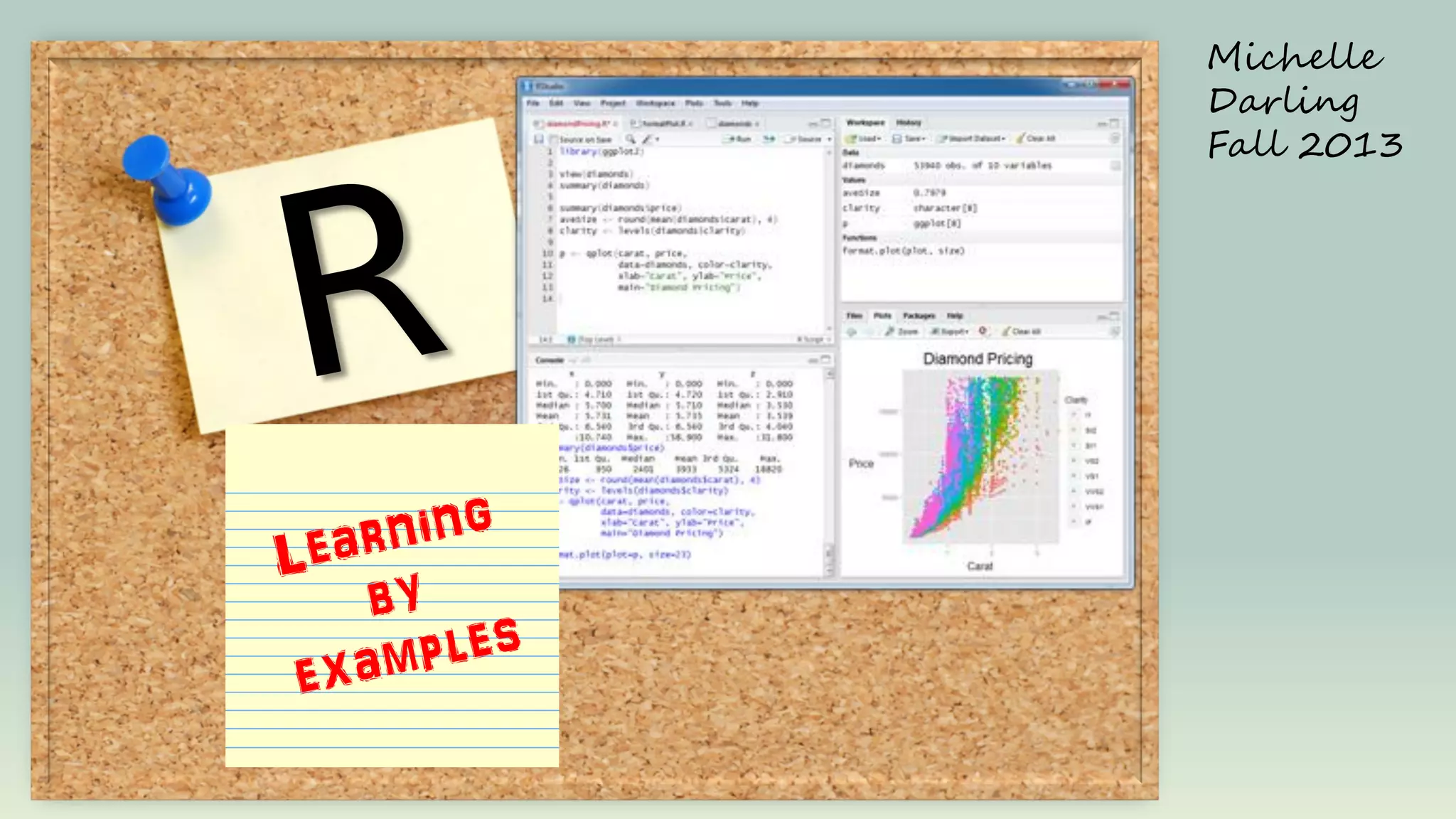
4. VECTOR:
Examples
[1]
[2]
[3]

5. VECTORS
[1]
[2]
[3]
# 1xN array of same data type
> v<-c(1:3); v
[1] 1 2 3
> mode(v)
# displays data type
[1] "numeric"
> v <-c("one", "two", "three"); v
[1] "one"
"two"
"three"
> mode(v)
[1] "character"
> v <-c(TRUE,FALSE,TRUE); v
[1] TRUE FALSE TRUE
> mode(v)
[1] "logical"
> v<-c(pi, 2*pi, 3*pi); v
[1] 3.141593 6.283185 9.424778
> mode(v)
[1] "numeric"
# Numeric values coerced into character mode
> v<-c(1,2,3,"one", "two", "three"); v
[1] "1"
"2"
"3"
"one"
"two"
"three"
> mode(v)
[1] "character"
BASIC OPERATIONS
# Addition
> v1<-1:3
> v2 <- c(10,10,10)
> mode(v1)
[1] "numeric"
> mode(v2)
[1] "numeric"
> v1+v2
[1] 11 12 13
# Multiplication &
Division
> v1 * v2
[1] 10 20 30
> v1 / v2
[1] 0.1 0.2 0.3
> v2 / v1
[1] 10.000000 5.000000
3.333333
#Subtraction
> v1-v2
[1] -9 -8 -7
> v2-v1
[1] 9 8 7
# Logical Comparison
> v1==v2
[1] FALSE FALSE FALSE
> v1 != v2
[1] TRUE TRUE TRUE
> v1 > v2
[1] FALSE FALSE FALSE
> v1 < v2
[1] TRUE TRUE TRUE

6. VECTORS
[1]
[2]
[3]
# By default, column numbers are used as indexes
> v3[1]
[1] 1
# But columns can be given meaningful names…
> names(v3) # What are current column names?
NULL
> names(v3)<- c("1st","2nd","3rd","4th","5th",
"6th") # Rename column names.
> names(v3) [1] "1st" "2nd" "3rd" "4th" "5th"
"6th"
> v3
1st 2nd 3rd 4th 5th 6th
1
2
3 10 10 10
# Now we can use names as indexes:
> v3["6th"] # same as v3[6]
6th
10
> v3[c("1st","6th")] # same as v3[c(1,6)]
1st 6th
1 10
> v3[-1] # Can exclude columns using (-)
2nd 3rd 4th 5th 6th
2
3 10 10 10
INDEXING, SELECTING
& SUBSETTING
> v3[v3==10] # Select values equal to 10
[1] 10 10 10
> v3[v3!=10] # Select values NOT equal to 10
[1] 1 2 3
> median(v3)
[1] 6.5
> v3[v3<median(v3)] # Select values < median
[1] 1 2 3
> v3[v3>median(v3)] # Select values > median
[1] 10 10 10
> v3 < median(v3) # Test if value < median?
[1] TRUE TRUE TRUE FALSE FALSE FALSE
> v3 %% 2==0 # Test if value is an even number?
[1] FALSE TRUE FALSE TRUE TRUE TRUE
> v3 %% 2==1 # Test if value is an odd number?
[1] TRUE FALSE TRUE FALSE FALSE FALSE

7. LIST:
Examples
[1]
[2]
Product Details








Series: O'Reilly Cookbooks
Paperback: 438 pages
Publisher: O'Reilly Media; 1 edition (March 22, 2011)
Language: English
ISBN-10: 0596809158
ISBN-13: 978-0596809157
Product Dimensions: 0.9 x 7 x 9.2 inches
Shipping Weight: 1.6 pounds
[3]

8. LISTS
[[1]]
[[2]]
[[3]]
# 1xN array of multiple data types/modes
> c1 <-c("A", "B", "C")
> n1 <-c(1:3)
> l2 <- list(c1,n1,Sys.Date(),TRUE);l2
[[1]]
[1] "A" "B" "C"
[[2]]
[1] 1 2 3
[[3]]
[1] "2013-11-03"
[[4]]
[1] TRUE
> str(l2)
List of 4
$ : chr [1:3] "A" "B" "C"
$ : int [1:3] 1 2 3
$ : Date[1:1], format: "2013-11-03"
$ : logi TRUE
> l2[[4]]
[1] TRUE
> l2[[1]]
[1] "A" "B" "C"
------->fix('l2')
list(c("A", "B", "C"), 1:3, structure(16012, class =
"Date"),TRUE)
# Append to a list; the results get trippy
> l2 <- list(l2,pi); l2
[[1]]
[[1]][[1]]
[1] "A" "B" "C"
[[1]][[2]]
[1] 1 2 3
[[1]][[3]]
[1] "2013-11-03"
[[1]][[4]]
[1] TRUE
[[2]]
[1] 3.141593
# Basically, a new () gets added each time the list is
appended
list(list(c("A", "B", "C"), 1:3, structure(16012, class =
"Date"), TRUE), 3.14159265358979)
# [[1]] is not the same as [1]
> mode(l3[[1]])
[1] "numeric"
> mode(l3[1])
[1] "list"
# To avoid confusion, use names
> l3 = list(x=1,y=2,z=3); l3
$x
[1] 1
$y
[1] 2
$z
[1] 3
> l3$x # this is the same as l3[[1]]
[1] 1

9. MATRIX:
Examples
[,1]
[1,]
[2,]
[3,]
[,2]
[,3]
Recommendation
Engine
Matrices
bought bought bought
bought likely buy likely buy

10. DATA FRAME:
Examples
[,1]
[,2]
[,3]
[1,]
[2,]
[3,]
Data Frames: Most frequently used structure for storing and manipulating
data sets. Similar to:
• A database table
• A spreadsheet
Like the above, DFs have rows x columns, but terminology is different:
• Observations = rows
• Variables = Columns
R Table vs. Data Frame: KISS and stick to data frames for now.
#Convert table to data frame:
> HEC <- data.frame(HairEyeColor)
> str(HEC)
'data.frame':32 obs. of 4 variables:
$ Hair: Factor w/ 4 levels "Black","Brown",..: 1 2 3 4 1 2 3 4 1 2 ...
$ Eye : Factor w/ 4 levels "Brown","Blue",..: 1 1 1 1 2 2 2 2 3 3 ...
$ Sex : Factor w/ 2 levels "Male","Female": 1 1 1 1 1 1 1 1 1 1 ...
$ Freq: num 32 53 10 3 11 50 10 30 10 25 ...

11. DATA FRAMES
[,1]
[,2]
[,3]
[1,]
[2,]
[3,]
# HEC[1,] returns a row
> HEC[1,]
Hair
Eye Sex Freq
1 Black Brown Male
32
# Subsetting made easier
> HEC6 <-subset(HEC,select=Hair); str(HEC6)
'data.frame':
32 obs. of 1 variable:
$ Hair: Factor w/ 4 levels "Black","Brown",..: 1 2 3 4
> HEC7 <-subset(HEC,select= c(Hair,Eye)); str(HEC7)
'data.frame':
32 obs. of 2 variables:
$ Hair: Factor w/ 4 levels "Black","Brown"...
$ Eye : Factor w/ 4 levels "Brown","Blue"...
> HEC8 <-subset(HEC, subset=(Hair == "Black" & Eye ==
"Brown")); HEC8
Hair
Eye
Sex Freq
1 Black Brown
Male
32
17 Black Brown Female
36
INDEXING, SELECTING
& SUBSETTING
# HEC[[1]], HEC[,"Hair"], HEC$Hair return column
> HEC1 <-HEC[[1]]; HEC1
> str(HEC1)
Factor w/ 4 levels "Black","Brown",..: 1 2 3 4 1 2 3 4 1 2 ...
# HEC[1] and HEC["Hair"] return column dframe
> HEC2 <-HEC[1]; HEC2
> str(HEC2)
'data.frame':32 obs. of 1 variable:
$ Hair: Factor w/ 4 levels "Black","Brown",..: 1 2 3 4 1 2 3 4 1 2
> HEC4 <-HEC["Hair"]
> HEC2 == HEC4
Hair
[1,] TRUE
[2,] TRUE
#
#
>
>
etc.
Returning multiple columns in a data frame
This is the same as HEC[,c(1, 4)]
HEC5 <-HEC[,c("Hair", "Freq")]
str(HEC5)
'data.frame':
32 obs. of 2 variables:
$ Hair: Factor w/ 4 levels "Black","Brown",..: 1 2 3 4 1 2 3 4 1
$ Freq: num 32 53 10 3 11 50 10 30 10 25 ...

12. DATA FRAMES
# Combine 2 DFs columnwise
> echo <- cbind(HEC2, HEC4)
> echo
Hair Hair
1 Black Black
2 Brown Brown
3 Red
Red etc
# Stack 2 DFs (UNION)
> rbind(HEC8, HEC8)
1
17
11
171
Hair
Black
Black
Black
Black
Eye
Sex Freq
Brown
Male
32
Brown Female
36
Brown
Male
32
Brown Female
36
# Skip having to specify the DF for col names
> f <- sum(HEC$Freq)
# Instead of this
> attach(HEC)
> f <- sum(Freq) # Use this

13. FUNCTIONS
SEQUENCING
seq(from,to,by) generate a sequence
indices <- seq(1,10,2)
#indices is c(1, 3, 5, 7, 9)
rep(x,ntimes)
repeat x n times
y <- rep(1:3, 2)
# y is c(1, 2, 3, 1, 2, 3)
cut(x,n)
divide continuous variable in factor
with n levels
y <- cut(x, 5)
DATE PROCESSING
Sys.Date()
as.date()
generate today's date
> Sys.Date()
[1] "2013-11-03
Convert string to date format
> to=as.Date('2006-1-10')
> mode(to)
[1] "numeric"
> class(to)
[1] "Date"
CHARACTER PROCESSING Description
substr(x, start=n1, stop=n2)
Extract or replace substrings in a character vector.
x <- "abcdef"
substr(x, 2, 4) is "bcd"
substr(x, 2, 4) <- "22222" is "a222ef"
grep(pattern, x ,
Search for pattern in x. If fixed =FALSE then pattern is
ignore.case=FALSE, fixed=FALSE) a regular expression. If fixed=TRUE then pattern is a
text string. Returns matching indices.
grep("A", c("b","A","c"), fixed=TRUE) returns 2
sub(pattern, replacement,x,
Find pattern in x and replace with replacement text. If
ignore.case =FALSE, fixed=FALSE) fixed=FALSE then pattern is a regular expression.
If fixed = T then pattern is a text string.
sub("s",".","Hello There") returns "Hello.There"
strsplit(x, split)
Split the elements of character vector x at split.
strsplit("abc", "") returns 3 element vector "a","b","c"
paste(..., sep="")
Concatenate strings after using sep string to seperate
them.
paste("x",1:3,sep="") returns c("x1","x2" "x3")
paste("x",1:3,sep="M") returns c("xM1","xM2" "xM3")
paste("Today is", date())
toupper(x)
Uppercase
tolower(x)
Lowercase
TYPE CONVERSION
STRUCTURE CONVERSION
as.character(x)
as.complex(x)
as.numeric(x)
as.logical(x)
as.data.frame(x)
as.list(x)
as.matrix(x)
as.vector(x)

14. DATA TRANSFORMATIONS
VECTOR
[1]
[2]
[3]
MATRIX
# s=simplify into a vector
# sapply returns a vector
l <- sapply(lst,function)
# lapply returns a list
v <- lapply(lst,function)
[,1]
[,3]
[1,]
[2,]
[3,]
DATA FRAME
LIST
[1]
[,2]
[2]
[,1]
[3]
[1,]
[2,]
[3,]
[,2]
[,3]

15. GET HELPFUL INFO
PRINTING
# Get help
>help.search("cat") # find info about "cat"
>?mean # get help about function
>example(mean) # get examples
> print(matrix(c(1234),2,2))
[,1] [,2]
[1,] 1234 1234
[2,] 1234 1234
# List objects in workspace
> ls()
[1] "tbl"
"w_day"
> print(matrix(c(1,2,3,4),2,2))
[,1] [,2]
[1,]
1
3
[2,]
2
4
# List all available datasets
> data()
# Get structure
> str(HairEyeColor)
table [1:4, 1:4, 1:2] 32 53 10 3 11 50 10 30 10 25
...
- attr(*, "dimnames")=List of 3
..$ Hair: chr [1:4] "Black" "Brown" "Red" "Blond"
..$ Eye : chr [1:4] "Brown" "Blue" "Hazel" "Green"
..$ Sex : chr [1:2] "Male" "Female"
# Get Class (vector,list, dataframe, table, matrix,
numeric, function, factor,, et)
> class(HairEyeColor)
[1] "table"
# Use Google R style sheet
> print ("print works on only");print("one
string or variable at a time"); print(pi)
[1] "print works on only"
[1] "one string or variable at a time"
[1] 3.141593
> num <-1:10
> print(num)
[1] 1 2 3
4
5
6
7
8
9 10
# cat works only on strings and vectors
> cat("the first 10 numbers are:", num, "n")
the first 10 numbers are: 1 2 3 4 5 6 7 8 9 10

16. INPUT / OUTPUT
Ctrl-R executes the selected line(s)
# Getting and setting the working directory
> getwd()
[1] "C:/Users/mdarling/Documents"
> setwd("DA/data")
[1] "C:/Users/mdarling/Documents/DA/data"
# Enter data using spreadsheet editor
w_day <- data.frame()
w_day <- edit(w_day)
# Read data from URL
> tbl <read.csv("http://www.andrewpatton.com/countrylist.csv")
# Write data to csv file
> write.csv(tbl, "countries.csv")
#
>
>
>
Read data from HTML tables
library(XML)
url <-"http://www.andrewpatton.com/countrylist.html"
tbls <- readHTMLTable(url)
MORE DATE PROCESSING
library(timeDate)
ymdhs <- "2012-03-04 05:06:07"
pd.sec <- as.POSIXlt(ymdhs)$sec
pd.hour <- as.POSIXlt(ymdhs)$hour
pd.min <- as.POSIXlt(ymdhs)$min
pd.mday <- as.POSIXlt(ymdhs)$mday
pd.mon <- ((as.POSIXlt(ymdhs)$mon)+1)
pd.year <- ((as.POSIXlt(ymdhs)$year) + 1900)

17. PLOTTING
Plotting in R
- base
- ggplot2, ggmap, map
Types of Graphs
- chloropleth
- heat map
# Base plots
plot(faithful, type = 'l') #line graph
plot(faithful, type = 'p') #point graph
hist(faithful$waiting)
#histogram of column waiting
# Quickly plot a matrix of scatterplots
# This plots each column vs. all the other ones
names(iris)
[1] "Sepal.Length" "Sepal.Width" "Petal.Length"
"Petal.Width" "Species"
pairs(iris[,-5])
pairs(iris[,1:2])
# Plot x vs. y using 2 df columnns and geom_point()
ggplot(movies, aes(x=year, y=budget)) + geom_point()
# Plot histogram using 1 column, Note: geom_bar()
ggplot(movies, aes(x=year)) + geom_bar()
# plot all rows vs. mpaa column
plot(movies[, "mpaa"]) # plot has lots of nulls
mpaa.movies <- subset(movies, mpaa != "")! # exclude nulls
plot(mpaa.movies[, "mpaa"])
# Or use na.rm