PROCESS SCHEDULING.pptx in operating system

Basic concepts
• Scheduling is the basis of multiprogrammed operating systems. By
switching the CPU among processes, the operating system can make
the computer more productive.
• In a single-processor system, only one process can run at a time.
Others must wait until the CPU is free and can be rescheduled.
• The objective of multiprogramming is to have some process running
at all times, to maximize CPU utilization.
• A process is executed until it must wait, typically for the completion of
some I/O request. In a simple computer system, the CPU then just sits
idle. All this waiting time is wasted; no useful work is accomplished

• When one process has to wait, the operating system takes the CPU away from that process and gives
the CPU to another process. This pattern continues. Every time one process has to wait, another
process can take over use of the CPU
• Scheduling is the process of controlling and prioritizing processes to send to a processor for
execution. The goal of scheduling is maintaining a constant amount of work for the processor,
eliminating high and lows in the workload and making sure each process is completed within a
reasonable time frame. It is an internal operating system program, called the scheduler performs this
task.
• CPU scheduling is done in the following four circumstances:
When a process switches from the running state to the waiting state
When a process switches from the running state to the ready state (For example, when an interrupt
occurs)
When process switches from the waiting state to the ready state (For example, at completion of I/O)
When a process terminates.

• Technical terms used in scheduling:
Ready queue: The processes waiting to be assigned to a processor are
put in a queue called ready queue.
Burst time: The time for which a process holds the CPU is known as
burst time.
Arrival time: Arrival Time is the time at which a process arrives at the
ready queue.
Turnaround time: The interval from the time of submission of a
process to the time of completion is the turnaround time.

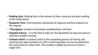
• Waiting time: Waiting time is the amount of time a process has been waiting
in the ready queue.
• Response Time: Time between submission of requests and first response to
the request
• Throughput: number of processes completed per unit time.
• Dispatch latency – It is the time it takes for the dispatcher to stop one process
and start another running
• Context switch: A context switch is the computing process of storing and
restoring the state (context) of a CPU so that execution can be resumed from
the same point at a later time. This enables multiple processes to share a
single CPU.

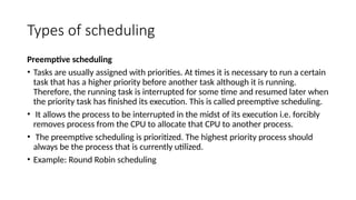
Types of scheduling
Preemptive scheduling
• Tasks are usually assigned with priorities. At times it is necessary to run a certain
task that has a higher priority before another task although it is running.
Therefore, the running task is interrupted for some time and resumed later when
the priority task has finished its execution. This is called preemptive scheduling.
• It allows the process to be interrupted in the midst of its execution i.e. forcibly
removes process from the CPU to allocate that CPU to another process.
• The preemptive scheduling is prioritized. The highest priority process should
always be the process that is currently utilized.
• Example: Round Robin scheduling

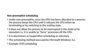
Non preemptive scheduling
• Under non-preemptive, once the CPU has been allocated to a process,
the process keeps the CPU until it releases the CPU either by
terminating or by switching to the waiting state.
• It does not allow the process to be interrupted in the midst of its
execution i.e. it is unable to "force" processes off the CPU.
• It is also known as Cooperative scheduling or voluntary.
• This scheduling method was used by Microsoft Windows 3.x.
• Example: FCFS scheduling

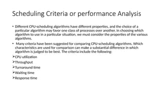
Scheduling Criteria or performance Analysis
• Different CPU-scheduling algorithms have different properties, and the choice of a
particular algorithm may favor one class of processes over another. In choosing which
algorithm to use in a particular situation, we must consider the properties of the various
algorithms.
• Many criteria have been suggested for comparing CPU-scheduling algorithms. Which
characteristics are used for comparison can make a substantial difference in which
algorithm is judged to be best. The criteria include the following:
CPU utilization
Throughput
Turnaround time
Waiting time
Response time

• CPU utilization. We want to keep the CPU as busy as possible. Conceptually, CPU
utilization can range from 0 to 100 percent. In a real system, it should range from
40 percent (for a lightly loaded system) to 90 percent (for a heavily loaded system).
• Throughput. If the CPU is busy executing processes, then work is being done. One
measure of work is the number of processes that are completed per time unit,
called throughput. For long processes, this rate may be one process per hour; for
short transactions, it may be ten processes per second.
• Turnaround time. From the point of view of a particular process, the important
criterion is how long it takes to execute that process. The interval from the time of
submission of a process to the time of completion is the turnaround time.
Turnaround time is the sum of the periods spent waiting to get into memory,
waiting in the ready queue, executing on the CPU, and doing I/O.

• Waiting time. The CPU-scheduling algorithm does not affect the amount of
time during which a process executes or does I/O. It affects only the amount
of time that a process spends waiting in the ready queue. Waiting time is the
sum of the periods spent waiting in the ready queue.
• Response time. In an interactive system, turnaround time may not be the
best criterion. Often, a process can produce some output fairly early and can
continue computing new results while previous results are being output to
the user. Thus, another measure is the time from the submission of a request
until the first response is produced. This measure, called response time, is the
time it takes to start responding, not the time it takes to output the response.
The turnaround time is generally limited by the speed of the output device.

Categories of Scheduling Algorithms
• In different environments different scheduling algorithms are needed.
This situation arises because different application areas (and different
kinds of operating systems) have different goals. In other words, what
the scheduler should optimize for is not the same in all systems. Three
environments worth distinguishing are
1. Batch.
2. Interactive.
3. Real time.

• Batch Scheduling: Batch scheduling is a way for computers to process a set of
tasks without requiring constant user interaction. In a batch system, a series of
jobs or tasks are executed one after the other without the need for immediate
user input. The focus is on maximizing efficiency and throughput.
• Interactive Scheduling: Interactive scheduling is a method used by computers
to quickly respond to user inputs or requests while they are actively using the
system. The goal is to provide a responsive and interactive experience by sharing
the CPU time among different tasks, ensuring that users don't experience
significant delays.
• Real-Time Scheduling: Real-time scheduling is a strategy employed in computer
systems to ensure that tasks are completed within specific deadlines, especially
in critical applications where timing is crucial. Real-time systems aim to meet
strict timing requirements, and scheduling algorithms are designed to prioritize
and execute tasks according to their urgency and deadlines.

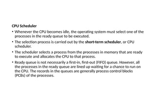
CPU Scheduler
• Whenever the CPU becomes idle, the operating system must select one of the
processes in the ready queue to be executed.
• The selection process is carried out by the short-term scheduler, or CPU
scheduler.
• The scheduler selects a process from the processes in memory that are ready
to execute and allocates the CPU to that process.
• Ready queue is not necessarily a first-in, first-out (FIFO) queue. However, all
the processes in the ready queue are lined up waiting for a chance to run on
the CPU. The records in the queues are generally process control blocks
(PCBs) of the processes.

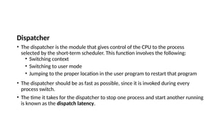
Dispatcher
• The dispatcher is the module that gives control of the CPU to the process
selected by the short-term scheduler. This function involves the following:
• Switching context
• Switching to user mode
• Jumping to the proper location in the user program to restart that program
• The dispatcher should be as fast as possible, since it is invoked during every
process switch.
• The time it takes for the dispatcher to stop one process and start another running
is known as the dispatch latency.

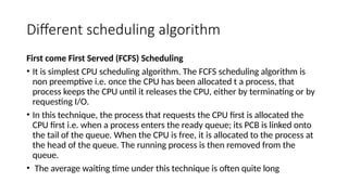
Different scheduling algorithm
First come First Served (FCFS) Scheduling
• It is simplest CPU scheduling algorithm. The FCFS scheduling algorithm is
non preemptive i.e. once the CPU has been allocated t a process, that
process keeps the CPU until it releases the CPU, either by terminating or by
requesting I/O.
• In this technique, the process that requests the CPU first is allocated the
CPU first i.e. when a process enters the ready queue; its PCB is linked onto
the tail of the queue. When the CPU is free, it is allocated to the process at
the head of the queue. The running process is then removed from the
queue.
• The average waiting time under this technique is often quite long

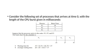
• Consider the following set of processes that arrives at time 0, with the
length of the CPU burst given in milliseconds:

• Suppose that the process arrive in the order P2,P3,P1
• The gantt chart for the schedule is

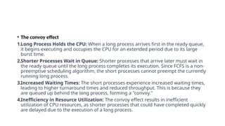
• The convoy effect
1.Long Process Holds the CPU: When a long process arrives first in the ready queue,
it begins executing and occupies the CPU for an extended period due to its large
burst time.
2.Shorter Processes Wait in Queue: Shorter processes that arrive later must wait in
the ready queue until the long process completes its execution. Since FCFS is a non-
preemptive scheduling algorithm, the short processes cannot preempt the currently
running long process.
3.Increased Waiting Times: The short processes experience increased waiting times,
leading to higher turnaround times and reduced throughput. This is because they
are queued up behind the long process, forming a "convoy."
4.Inefficiency in Resource Utilization: The convoy effect results in inefficient
utilization of CPU resources, as shorter processes that could have completed quickly
are delayed due to the execution of a long process.

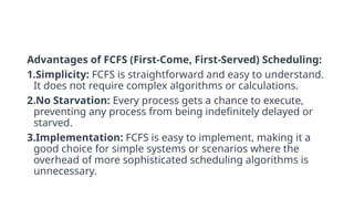
Advantages of FCFS (First-Come, First-Served) Scheduling:
1.Simplicity: FCFS is straightforward and easy to understand.
It does not require complex algorithms or calculations.
2.No Starvation: Every process gets a chance to execute,
preventing any process from being indefinitely delayed or
starved.
3.Implementation: FCFS is easy to implement, making it a
good choice for simple systems or scenarios where the
overhead of more sophisticated scheduling algorithms is
unnecessary.

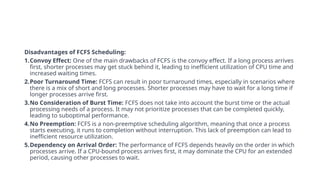
Disadvantages of FCFS Scheduling:
1.Convoy Effect: One of the main drawbacks of FCFS is the convoy effect. If a long process arrives
first, shorter processes may get stuck behind it, leading to inefficient utilization of CPU time and
increased waiting times.
2.Poor Turnaround Time: FCFS can result in poor turnaround times, especially in scenarios where
there is a mix of short and long processes. Shorter processes may have to wait for a long time if
longer processes arrive first.
3.No Consideration of Burst Time: FCFS does not take into account the burst time or the actual
processing needs of a process. It may not prioritize processes that can be completed quickly,
leading to suboptimal performance.
4.No Preemption: FCFS is a non-preemptive scheduling algorithm, meaning that once a process
starts executing, it runs to completion without interruption. This lack of preemption can lead to
inefficient resource utilization.
5.Dependency on Arrival Order: The performance of FCFS depends heavily on the order in which
processes arrive. If a CPU-bound process arrives first, it may dominate the CPU for an extended
period, causing other processes to wait.

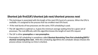
Shortest job first(SJF)/shortest job next/shortest process next
• This technique is associated with the length of the next CPU burst of a process. When the CPU is
available, it is assigned to the process that has smallest next CPU burst.
• If the next bursts of two processes are the same, FCFS scheduling is used.
• The SJF algorithm is optimal i.e. it gives the minimum average waiting time for a given set of
processes. The real difficulty with this algorithm knows the length of next CPU request
• The SJF is either preemptive or non preemptive.
• Preemptive SJF scheduling is sometimes called Shortest Remaining Time First scheduling(SRTF)/
shortest remaining time next.. With this scheduling algorithms the scheduler always chooses the
process whose remaining run time is shortest.

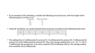
• As an example of SJF scheduling, consider the following set of processes, with the length of the
CPU burst given in milliseconds
• Using SJF scheduling, we would schedule these processes according to the following Gantt chart
• The waiting time is 3 milliseconds for process P1, 16 milliseconds for process P2, 9 milliseconds for
process P3, and 0 milliseconds for process P4. Thus, the average waiting time is (3 + 16 + 9 + 0)/4 =
7 milliseconds. By comparison, if we were using the FCFS scheduling scheme, the average waiting
time would be 10.25 milliseconds.

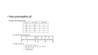
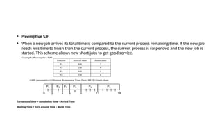
• Preemptive SJF
• When a new job arrives its total time is compared to the current process remaining time. If the new job
needs less time to finish than the current process, the current process is suspended and the new job is
started. This scheme allows new short jobs to get good service.
Turnaround time = completion time – Arrival Time
Waiting Time = Turn around Time – Burst Time

• Average Turn around Time = [(16-0) +(7-2) + (5-4) + (11-5)] / 4
= 7ms
• Average waiting time = [(11 – 2) + (5 – 4) + (4 – 4) + (7 – 5)] / 4
= (9 + 1 + 0 +2) / 4
= 3 milliseconds

Draw gantt chart and calculate the average waiting time and
turn around time
Calculate average waiting time and average turn around
time?????
Gantt chart

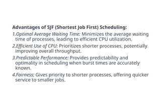
Advantages of SJF (Shortest Job First) Scheduling:
1.Optimal Average Waiting Time: Minimizes the average waiting
time of processes, leading to efficient CPU utilization.
2.Efficient Use of CPU: Prioritizes shorter processes, potentially
improving overall throughput.
3.Predictable Performance: Provides predictability and
optimality in scheduling when burst times are accurately
known.
4.Fairness: Gives priority to shorter processes, offering quicker
service to smaller jobs.

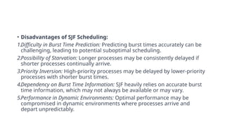
• Disadvantages of SJF Scheduling:
1.Difficulty in Burst Time Prediction: Predicting burst times accurately can be
challenging, leading to potential suboptimal scheduling.
2.Possibility of Starvation: Longer processes may be consistently delayed if
shorter processes continually arrive.
3.Priority Inversion: High-priority processes may be delayed by lower-priority
processes with shorter burst times.
4.Dependency on Burst Time Information: SJF heavily relies on accurate burst
time information, which may not always be available or may vary.
5.Performance in Dynamic Environments: Optimal performance may be
compromised in dynamic environments where processes arrive and
depart unpredictably.

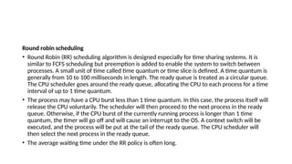
Round robin scheduling
• Round Robin (RR) scheduling algorithm is designed especially for time sharing systems. It is
similar to FCFS scheduling but preemption is added to enable the system to switch between
processes. A small unit of time called time quantum or time slice is defined. A time quantum is
generally from 10 to 100 milliseconds in length. The ready queue is treated as a circular queue.
The CPU scheduler goes around the ready queue, allocating the CPU to each process for a time
interval of up to 1 time quantum.
• The process may have a CPU burst less than 1 time quantum. In this case, the process itself will
release the CPU voluntarily. The scheduler will then proceed to the next process in the ready
queue. Otherwise, if the CPU burst of the currently running process is longer than 1 time
quantum, the timer will go off and will cause an interrupt to the OS. A context switch will be
executed, and the process will be put at the tail of the ready queue. The CPU scheduler will
then select the next process in the ready queue.
• The average waiting time under the RR policy is often long.

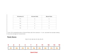
If we use time quantum of 4ms then gantt chart is given as
below

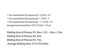
• Turn around time for process p1 = (27-0) = 27
• Turn around time for process p2 = (7-0) = 7
• Turn around time for process p3 = ( 11-0) = 11
Average turnaround time =(27+7+11)/3 = 15 ms
Waiting time of Process P1: 0ms + (11 – 4)ms = 7ms
Waiting time of Process P2: 4ms
Waiting time of Process P3: 7ms
Average Waiting time: (7+4+7)/3=6ms

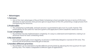
• Advantages:
1.Fairness:
1. One of the main advantages of Round Robin Scheduling is that it provides fairness in terms of CPU time
allocation to each process. Every process gets an equal share of the CPU, preventing a single process from
monopolizing the resources.
2.Predictable:
1. The scheduling is predictable, and each process is guaranteed to get a turn in a cyclic manner. This
predictability can be useful for real-time systems and applications where deadlines need to be met.
3.Low complexity:
1. Round Robin has low implementation complexity. It is easy to understand and implement, making it an
attractive choice for basic scheduling needs.
4.No starvation:
1. Since each process gets a turn regularly, no process is indefinitely delayed or starved of CPU time. This
ensures that all processes eventually get to execute.
5.Handles different priorities:
1. Round Robin can be extended to handle different priority levels by adjusting the time quantum for each
priority class. This makes it adaptable to different types of applications.

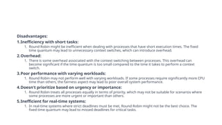
Disadvantages:
1.Inefficiency with short tasks:
1. Round Robin might be inefficient when dealing with processes that have short execution times. The fixed
time quantum may lead to unnecessary context switches, which can introduce overhead.
2.Overhead:
1. There is some overhead associated with the context switching between processes. This overhead can
become significant if the time quantum is too small compared to the time it takes to perform a context
switch.
3.Poor performance with varying workloads:
1. Round Robin may not perform well with varying workloads. If some processes require significantly more CPU
time than others, the fairness aspect may lead to poor overall system performance.
4.Doesn't prioritize based on urgency or importance:
1. Round Robin treats all processes equally in terms of priority, which may not be suitable for scenarios where
some processes are more urgent or important than others.
5.Inefficient for real-time systems:
1. In real-time systems where strict deadlines must be met, Round Robin might not be the best choice. The
fixed time quantum may lead to missed deadlines for critical tasks.

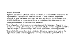
• Priority scheduling
• A priority is associated with each process, and the CPU is allocated to the process with the
highest priority. Equal priorities are scheduled in FCFS order. Priorities are generally
indicated by some fixed range of numbers and there is no general method of indicating
which is the highest or lowest priority, it may be either increasing or decreasing order.
• Priority can be defined either internally or externally.
 Internally defined priorities use some measurable quantity to compute the priority of a
process. For example, time limits, memory requirements, the number of open files and the
ratio of average I/O burst to average CPU burst has been used in computing priorities.
External priorities are set by criteria outside the OS, such as importance of process, the
type and amount of funds being paid for computer user, and other political factors.

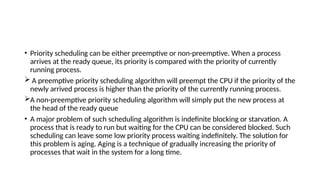
• Priority scheduling can be either preemptive or non-preemptive. When a process
arrives at the ready queue, its priority is compared with the priority of currently
running process.
 A preemptive priority scheduling algorithm will preempt the CPU if the priority of the
newly arrived process is higher than the priority of the currently running process.
A non-preemptive priority scheduling algorithm will simply put the new process at
the head of the ready queue
• A major problem of such scheduling algorithm is indefinite blocking or starvation. A
process that is ready to run but waiting for the CPU can be considered blocked. Such
scheduling can leave some low priority process waiting indefinitely. The solution for
this problem is aging. Aging is a technique of gradually increasing the priority of
processes that wait in the system for a long time.

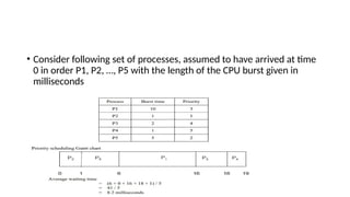
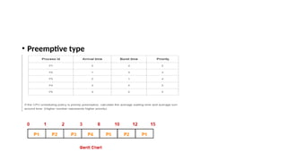
• Consider following set of processes, assumed to have arrived at time
0 in order P1, P2, …, P5 with the length of the CPU burst given in
milliseconds

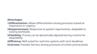
Advantages:
1.Differentiation: Allows differentiation among processes based on
importance or urgency.
2.Responsiveness: Responsive to system requirements, adaptable to
varying workloads.
3.Flexibility: Priority can be dynamically adjusted during runtime for
adaptability.
4.Efficiency: Well-suited for real-time systems with strict deadlines.
5.Fairness: Provides fairness among processes of similar priority levels.

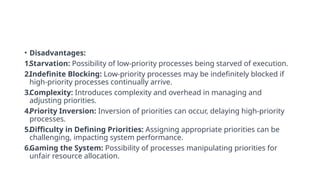
• Disadvantages:
1.Starvation: Possibility of low-priority processes being starved of execution.
2.Indefinite Blocking: Low-priority processes may be indefinitely blocked if
high-priority processes continually arrive.
3.Complexity: Introduces complexity and overhead in managing and
adjusting priorities.
4.Priority Inversion: Inversion of priorities can occur, delaying high-priority
processes.
5.Difficulty in Defining Priorities: Assigning appropriate priorities can be
challenging, impacting system performance.
6.Gaming the System: Possibility of processes manipulating priorities for
unfair resource allocation.

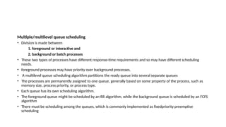
Multiple/multilevel queue scheduling
• Division is made between
1. foreground or interactive and
2. background or batch processes
• These two types of processes have different response-time requirements and so may have different scheduling
needs.
• foreground processes may have priority over background processes.
• A multilevel queue scheduling algorithm partitions the ready queue into several separate queues
• The processes are permanently assigned to one queue, generally based on some property of the process, such as
memory size, process priority, or process type.
• Each queue has its own scheduling algorithm.
• The foreground queue might be scheduled by an RR algorithm, while the background queue is scheduled by an FCFS
algorithm
• There must be scheduling among the queues, which is commonly implemented as fixedpriority preemptive
scheduling

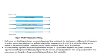
Figure Multilevel queue scheduling.
• Each queue has absolute priority over lower priority queues. No process can in the batch queue, could run unless the queues
for system process, interactive process, and interactive editing processes were all empty. If an interactive editing process
entered in the ready queue while a batch process was running, the batch process would be preempted.
• In such scheduling algorithm, processes are permanently assigned to a queue when they enter the system. If there are
separate queues foreground and background processes, for example, process do not move from one queue to another, since
processes do not change their foreground and background nature. So it is inflexible.

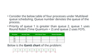
• Consider the below table of four processes under Multilevel
queue scheduling. Queue number denotes the queue of the
process.
• Priority of queue 1 is greater than queue 2. queue 1 uses
Round Robin (Time Quantum = 2) and queue 2 uses FCFS.
Below is the Gantt chart of the problem:

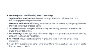
• Advantages of Multilevel Queue Scheduling:
1.Improved Responsiveness: Ensures prompt attention to interactive tasks,
enhancing system responsiveness.
2.Resource Utilization: Efficiently allocates system resources by assigning different
priorities to various process types.
3.Fairness: Provides a degree of fairness by preventing complete starvation of
lower-priority processes.
4.Adaptability: Allows dynamic adjustment of process priorities based on behavior,
adapting to changing workloads.
5.Prioritization: Supports assigning higher priorities to critical or real-time
processes.
6.Flexibility: Customizable scheduling algorithms within each queue accommodate
diverse process needs.

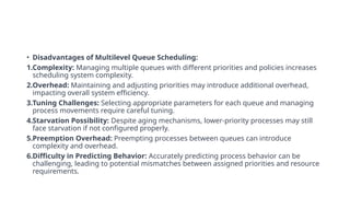
• Disadvantages of Multilevel Queue Scheduling:
1.Complexity: Managing multiple queues with different priorities and policies increases
scheduling system complexity.
2.Overhead: Maintaining and adjusting priorities may introduce additional overhead,
impacting overall system efficiency.
3.Tuning Challenges: Selecting appropriate parameters for each queue and managing
process movements require careful tuning.
4.Starvation Possibility: Despite aging mechanisms, lower-priority processes may still
face starvation if not configured properly.
5.Preemption Overhead: Preempting processes between queues can introduce
complexity and overhead.
6.Difficulty in Predicting Behavior: Accurately predicting process behavior can be
challenging, leading to potential mismatches between assigned priorities and resource
requirements.

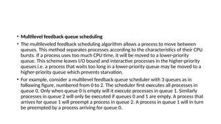
• Multilevel feedback queue scheduling
• The multileveled feedback scheduling algorithm allows a process to move between
queues. This method separates processes according to the characteristics of their CPU
bursts. If a process uses too much CPU time, it will be moved to a lower-priority
queue. This scheme leaves I/O bound and interactive processes in the higher-priority
queues i.e. a process that waits too long in a lower-priority queue may be moved to a
higher-priority queue which prevents starvation.
• For example, consider a multilevel feedback queue scheduler with 3 queues as in
following figure, numbered from 0 to 2. The scheduler first executes all processes in
queue 0. Only when queue 0 is empty will it execute processes in queue 1. Similarly
processes in queue 2 will only be executed if queues 0 and 1 are empty. A process that
arrives for queue 1 will preempt a process in queue 2. A process in queue 1 will in turn
be preempted by a process arriving for queue 0.

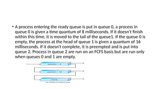
• A process entering the ready queue is put in queue 0, a process in
queue 0 is given a time quantum of 8 milliseconds. If it doesn't finish
within this time, it is moved to the tail of the queue1. If the queue 0 is
empty, the process at the head of queue 1 is given a quantum of 16
milliseconds. If it doesn't complete, it is preempted and is put into
queue 2. Process in queue 2 are run on an FCFS basis but are run only
when queues 0 and 1 are empty.

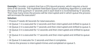
Example: Consider a system that has a CPU-bound process, which requires a burst
time of 40 seconds. The multilevel Feed Back Queue scheduling algorithm is used and
the queue time quantum ‘2’ seconds and in each level it is incremented by ‘5’ seconds.
Then how many times the process will be interrupted and in which queue the process
will terminate the execution?
Solution:
• Process P needs 40 Seconds for total execution.
• At Queue 1 it is executed for 2 seconds and then interrupted and shifted to queue 2.
• At Queue 2 it is executed for 7 seconds and then interrupted and shifted to queue 3.
• At Queue 3 it is executed for 12 seconds and then interrupted and shifted to queue
4.
• At Queue 4 it is executed for 17 seconds and then interrupted and shifted to queue
5.
• At Queue 5 it executes for 2 seconds and then it completes.
• Hence the process is interrupted 4 times and completed on queue 5.

Real time scheduling
• Real-time scheduling is a technique used in operating systems to manage and
schedule tasks with specific timing requirements. These tasks are often referred to as
real-time tasks, and they have deadlines or time constraints that must be met for the
system to function correctly. Real-time scheduling is crucial in systems where timely
and predictable execution of tasks is essential, such as in embedded systems,
industrial automation, robotics, and other time-sensitive applications.
• There are two main types of real-time scheduling: hard real-time scheduling and soft
real-time scheduling.
1.Hard Real-Time Scheduling:
1. In hard real-time systems, tasks have strict and non-negotiable deadlines that must be met.
2. Failure to meet a deadline can lead to catastrophic consequences.
3. Scheduling algorithms for hard real-time systems prioritize tasks based on their deadlines.
2.Soft Real-Time Scheduling:
1. In soft real-time systems, tasks have deadlines, but missing a deadline might not have severe
consequences.
2. The system aims to maximize the number of deadlines met, but occasional misses are
acceptable.
3. Scheduling algorithms for soft real-time systems often consider both deadlines and system
efficiency.

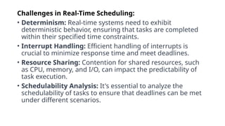
Challenges in Real-Time Scheduling:
• Determinism: Real-time systems need to exhibit
deterministic behavior, ensuring that tasks are completed
within their specified time constraints.
• Interrupt Handling: Efficient handling of interrupts is
crucial to minimize response time and meet deadlines.
• Resource Sharing: Contention for shared resources, such
as CPU, memory, and I/O, can impact the predictability of
task execution.
• Schedulability Analysis: It's essential to analyze the
schedulability of tasks to ensure that deadlines can be met
under different scenarios.

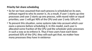
Priority fair share scheduling
• So far we have assumed that each process is scheduled on its own,
without regard to who its owner is. As a result, if user 1 starts up nine
processes and user 2 starts up one process, with round robin or equal
priorities, user 1 will get 90% of the CPU and user 2 only 10% of it.
• To prevent this situation, some systems take into account which user
owns a process before scheduling it. In this model, each user is
allocated some fraction of the CPU and the scheduler picks processes
in such a way as to enforce it. Thus if two users have each been
promised 50% of the CPU, they will each get that, no matter how
many processes they have in existence

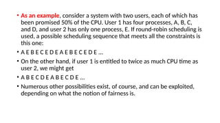
• As an example, consider a system with two users, each of which has
been promised 50% of the CPU. User 1 has four processes, A, B, C,
and D, and user 2 has only one process, E. If round-robin scheduling is
used, a possible scheduling sequence that meets all the constraints is
this one:
• A E B E C E D E A E B E C E D E ...
• On the other hand, if user 1 is entitled to twice as much CPU time as
user 2, we might get
• A B E C D E A B E C D E ...
• Numerous other possibilities exist, of course, and can be exploited,
depending on what the notion of fairness is.

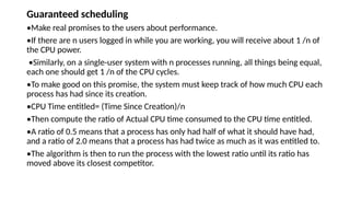
Guaranteed scheduling
•Make real promises to the users about performance.
•If there are n users logged in while you are working, you will receive about 1 /n of
the CPU power.
•Similarly, on a single-user system with n processes running, all things being equal,
each one should get 1 /n of the CPU cycles.
•To make good on this promise, the system must keep track of how much CPU each
process has had since its creation.
•CPU Time entitled= (Time Since Creation)/n
•Then compute the ratio of Actual CPU time consumed to the CPU time entitled.
•A ratio of 0.5 means that a process has only had half of what it should have had,
and a ratio of 2.0 means that a process has had twice as much as it was entitled to.
•The algorithm is then to run the process with the lowest ratio until its ratio has
moved above its closest competitor.

Lottery scheduling
• Lottery Scheduling is a probabilistic scheduling algorithm for processes in an
operating system. Processes are each assigned some number of lottery tickets for
various system resources such as CPU time.;and the scheduler draws a random ticket
to select the next process.
• The distribution of tickets need not be uniform; granting a process more tickets
provides it a relative higher chance of selection. This technique can be used to
approximate other scheduling algorithms, such as Shortest job next and Fairshare
scheduling.
• Lottery scheduling solves the problem of starvation. Giving each process at least one
lottery ticket guarantees that it has non-zero probability of being selected at each
scheduling operation. More important process can be given extra tickets to increase
their odd of winning.
• If there are 100 tickets outstanding, & one process holds 20 of them it will have 20%
chance of winning each lottery. In the long run it will get 20% of the CPU. A process
holding a fraction f of the tickets will get about a fraction of the resource in questions.

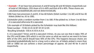
• Example – If we have two processes A and B having 60 and 40 tickets respectively out
of total of 100 tickets. CPU share of A is 60% and that of B is 40%. These shares are
calculated probabilistically and not deterministically.
1.We have two processes A and B. A has 60 tickets (ticket number 1 to 60) and B has 40
tickets (ticket no. 61 to 100).
2.Scheduler picks a random number from 1 to 100. If the picked no. is from 1 to 60 then
A is executed otherwise B is executed.
3.An example of 10 tickets picked by the Scheduler may look like this follows:
Ticket number - 73 82 23 45 32 87 49 39 12 09.
Resulting Schedule - B B A A A B A A A A.
4. A is executed 7 times and B is executed 3 times. As you can see that A takes 70% of
the CPU and B takes 30% which is not the same as what we need as we need A to have
60% of the CPU and B should have 40% of the CPU. This happens because shares are
calculated probabilistically but in a long run(i.e when no. of tickets picked is more than
100 or 1000) we can achieve a share percentage of approx. 60 and 40 for A and B
respectively.

Highest response ratio next(HRN) scheduling
• Highest Response Ratio Next (HRRN) scheduling is a non-preemptive discipline, in
which the priority of each job is dependent on its estimated run time, and also the
amount of time it has spent waiting.
• Jobs gain higher priority the longer they wait, which prevents indefinite postponement
(process starvation). It selects a process with the largest ratio of waiting time over
service time. This guarantees that a process does not starve due to its requirements.
In fact, the jobs that have spent a long time waiting compete against those estimated
to have short run times.
Priority = waiting time + estimated runtime / estimated runtime
(Or)
Ratio = (waiting time + service time) / service time

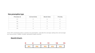
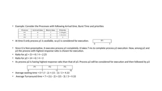
• Example: Consider the Processes with following Arrival time, Burst Time and priorities
• At time 0 only process p1 is available, so p1 is considered for execution.
• Since it is Non-preemptive, it executes process p1 completely. It takes 7 ms to complete process p1 execution. Now, among p2 and
p3 the process with highest response ratio is chosen for execution.
• Ratio for p2 = (5 + 4) / 4 = 2.25
• Ratio for p3 = (4 + 4) / 4 = 2
• As process p2 is having highest response ratio than that of p3. Process p2 will be considered for execution and then followed by p3
• Average waiting time = 0 + (7 - 2) + (11 - 3) / 3 = 4.33
• Average Turnaround time = 7 + (11 - 2) + (15 - 3) / 3 = 9.33

PROCESS SCHEDULING.pptx in operating system

More Related Content

Similar to PROCESS SCHEDULING.pptx in operating system

More from gautamb639

Recently uploaded

PROCESS SCHEDULING.pptx in operating system