Reasoning bayes rule conditional

1. ARTIFICIAL INTELLIGENCE
Lecturer: Silja Renooij
Uncertainty: probabilistic reasoning
Utrecht University
The Netherlands
These slides are part of the INFOB2KI Course Notes available from
www.cs.uu.nl/docs/vakken/b2ki/schema.html
INFOB2KI 2019-2020

2. Outline
 Reasoning under uncertainty
 Probabilities
 Bayes’ rule & Bayesian Networks
 Bayesian skill rating

3. Uncertainty
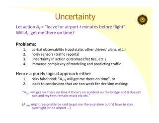
Let action At = “leave for airport t minutes before flight”
Will At get me there on time?
Problems:
1. partial observability (road state, other drivers' plans, etc.)
2. noisy sensors (traffic reports)
3. uncertainty in action outcomes (flat tire, etc.)
4. immense complexity of modeling and predicting traffic
Hence a purely logical approach either
1. risks falsehood: “A125 will get me there on time”, or
2. leads to conclusions that are too weak for decision making:
“A125 will get me there on time if there's no accident on the bridge and it doesn't
rain and my tires remain intact etc etc.”
(A1440 might reasonably be said to get me there on time but I'd have to stay
overnight in the airport …)

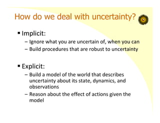
4. How do we deal with uncertainty?
 Implicit:
– Ignore what you are uncertain of, when you can
– Build procedures that are robust to uncertainty
 Explicit:
– Build a model of the world that describes
uncertainty about its state, dynamics, and
observations
– Reason about the effect of actions given the
model

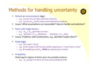
5. Methods for handling uncertainty
 Default or nonmonotonic logic:
– e.g. assume my car does not have a flat tire
– e.g. assume A125 works unless contradicted by evidence
 Issues: What assumptions are reasonable? How to handle contradiction?
 Rules with fudge factors:
– e.g. A125 |→0.3 get there on time;
– e.g. Sprinkler |→ 0.99 WetGrass; WetGrass |→ 0.7 Rain
 Issues: Problems with combination, e.g., Sprinkler implies Rain??
 Fuzzy Logic
– e.g. The road is “busy”
– e.g. At the airport 120 minutes before departure is “more than in time”
– e.g. IF road(busy) and A125 THEN at_airport (just‐in‐time)
 Probability
Model agent's degree of belief, given the available evidence
– e.g. A25 will get me there on time with probability 0.04

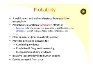
6. Probability
 A well‐known and well‐understood framework for
uncertainty
 Probabilistic assertions summarize effects of
– laziness: failure to enumerate exceptions, qualifications, etc.
– ignorance: lack of relevant facts, initial conditions, etc.
– …
 Clear semantics (mathematically correct)
 Provides principled answers for:
– Combining evidence
– Predictive & Diagnostic reasoning
– Incorporation of new evidence
 Intuitive (at some level) to human experts
 Can be assessed from data

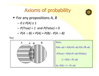
7. Axioms of probability
 For any propositions A, B
– 0 ≤ P(A) ≤ 1
– P(True) = 1 and P(False) = 0
– P(A  B) = P(A) + P(B) ‐ P(A  B)
Note:
P(AvA) = P(A)+P(A)‐P(A A)
P(True) = P(A)+P(A)‐P(False)
1 = P(A) + P(A)
So: P(A) = 1 ‐ P(A)

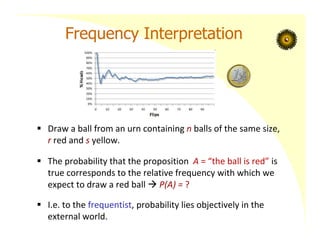
8. Frequency Interpretation
 Draw a ball from an urn containing n balls of the same size,
r red and s yellow.
 The probability that the proposition A = “the ball is red” is
true corresponds to the relative frequency with which we
expect to draw a red ball  P(A) = ?
 I.e. to the frequentist, probability lies objectively in the
external world.

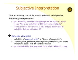
9. Subjective Interpretation
There are many situations in which there is no objective
frequency interpretation:
– On a windy day, just before paragliding from the top of El Capitan,
you say “there is a probability of 0.05 that I am going to die”
– You have worked hard on your AI class and you believe that the
probability that you will pass is 0.9
 Bayesian Viewpoint
– probability is "degree‐of‐belief", or "degree‐of‐uncertainty".
– To the Bayesian, probability lies subjectively in the mind, and can be
different for people with different information
– e.g., the probability that Wayne will get rich from selling his kidney.

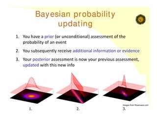
10. Bayesian probability
updating
1. You have a prior (or unconditional) assessment of the
probability of an event
2. You subsequently receive additional information or evidence
3. Your posterior assessment is now your previous assessment,
updated with this new info
Images from Moserware.com
1. 2. 3.

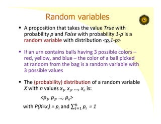
11. Random variables
 A proposition that takes the value True with
probability p and False with probability 1‐p is a
random variable with distribution <p,1‐p>
 If an urn contains balls having 3 possible colors –
red, yellow, and blue – the color of a ball picked
at random from the bag is a random variable with
3 possible values
 The (probability) distribution of a random variable
X with n values x1, x2, …, xn is:
<p1, p2, …, pn>
with P(X=xi) = pi and pi = 1

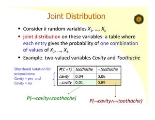
12. Joint Distribution
 Consider k random variables X1, …, Xk
 joint distribution on these variables: a table where
each entry gives the probability of one combination
of values of X1, …, Xk
 Example: two‐valued variables Cavity and Toothache
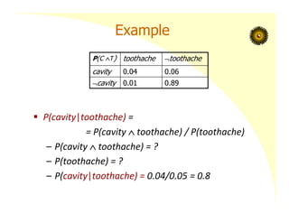
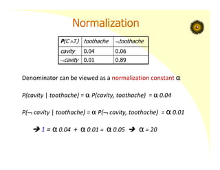
P(cavitytoothache)
P(cavitytoothache)
P(C T) toothache toothache
cavity 0.04 0.06
cavity 0.01 0.89
Shorthand notation for
propositions:
Cavity = yes and
Cavity = no

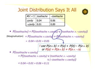
13. Joint Distribution Says It All
 P(toothache) = P((toothache  cavity) v (toothache  cavity))
= P(toothache  cavity) + P(toothache  cavity)
= 0.04 + 0.01 = 0.05
 P(toothache v cavity)
= P((toothache  cavity) v (toothache  cavity)
v (toothache  cavity))
= 0.04 + 0.01 + 0.06 = 0.11
P(C T) toothache toothache
cavity 0.04 0.06
cavity 0.01 0.89
! use P(a v b) = P(a) + P(b) – P(a  b)
or P(a) = P(a  b) + P(a   b)
(Marginalisation)

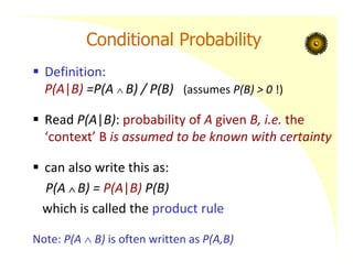
14. Conditional Probability
 Definition:
P(A|B) =P(A  B) / P(B) (assumes P(B) > 0 !)
 Read P(A|B): probability of A given B, i.e. the
‘context’ B is assumed to be known with certainty
 can also write this as:
P(A  B) = P(A|B) P(B)
which is called the product rule
Note: P(A  B) is often written as P(A,B)

15. Example
 P(cavity|toothache) =
= P(cavity  toothache) / P(toothache)
– P(cavity  toothache) = ?
– P(toothache) = ?
– P(cavity|toothache) = 0.04/0.05 = 0.8
P(C T) toothache toothache
cavity 0.04 0.06
cavity 0.01 0.89

16. Normalization
Denominator can be viewed as a normalization constant α
P(cavity | toothache) = α P(cavity, toothache) = α 0.04
P( cavity | toothache) = α P( cavity, toothache) = α 0.01
 1 = α 0.04 + α 0.01 = α 0.05  α = 20
P(C T) toothache toothache
cavity 0.04 0.06
cavity 0.01 0.89

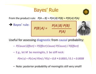
17. Bayes’ Rule
From the product rule: P(A  B) = P(A|B) P(B) = P(B|A) P(A)
 Bayes’ rule:
P(B|A) =
P(A|B) P(B)
P(A)
Useful for assessing diagnostic from causal probability:
– P(Cause|Effect) = P(Effect|Cause) P(Cause) / P(Effect)
– E.g., let M be meningitis, S be stiff neck:
P(m|s) = P(s|m) P(m) / P(s) = 0.8 × 0.0001 / 0.1 = 0.0008
– Note: posterior probability of meningitis still very small!

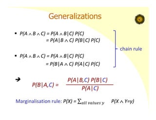
18. Generalizations
 P(A  B  C) = P(A  B|C) P(C)
= P(A|B  C) P(B|C) P(C)
 P(A  B  C) = P(A  B|C) P(C)
= P(B|A  C) P(A|C) P(C)

P(B|A,C) =
P(A|B,C) P(B|C)
P(A|C)
chain rule
Marginalisation rule: P(X) = P(X  Y=y)

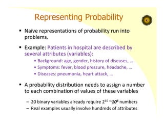
19. Representing Probability
 Naïve representations of probability run into
problems.
 Example: Patients in hospital are described by
several attributes (variables):
• Background: age, gender, history of diseases, …
• Symptoms: fever, blood pressure, headache, …
• Diseases: pneumonia, heart attack, …
 A probability distribution needs to assign a number
to each combination of values of these variables
– 20 binary variables already require 210 ~106 numbers
– Real examples usually involve hundreds of attributes

20. Practical Representation
 Key idea ‐‐ exploit regularities
 Here we focus on exploiting
(conditional) independence
properties

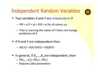
21. Independent Random Variables
 Two variables X and Y are independent if
– P(X = x|Y = y) = P(X = x) for all values x,y
– That is, learning the values of Y does not change
prediction of X
 If X and Y are independent then
– P(X,Y) = P(X|Y)P(Y) = P(X)P(Y)
 In general, if X1,…,Xn are independent, then
– P(X1,…,Xn)= P(X1)...P(Xn)
– Requires O(n) parameters

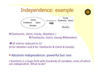
22. Independence: example
P(Toothache, Catch, Cavity, Weather) =
P(Toothache, Catch, Cavity) P(Weather)
32 entries reduced to 12
(4 for Weather and 8 for Toothache & Catch & Cavity);
 Absolute independence: powerful but rare
 Dentistry is a large field with hundreds of variables, none of which
are independent. What to do?

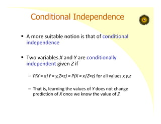
23. Conditional Independence
 A more suitable notion is that of conditional
independence
 Two variables X and Y are conditionally
independent given Z if
– P(X = x|Y = y,Z=z) = P(X = x|Z=z) for all values x,y,z
– That is, learning the values of Y does not change
prediction of X once we know the value of Z

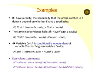
24. Examples
 If I have a cavity, the probability that the probe catches in it
doesn't depend on whether I have a toothache:
(1) P(catch | toothache, cavity) = P(catch | cavity)
 The same independence holds if I haven't got a cavity:
(2) P(catch | toothache, cavity) = P(catch | cavity)
  Variable Catch is conditionally independent of
variable Toothache given variable Cavity:
P(Catch | Toothache,Cavity) = P(Catch | Cavity)
 Equivalent statements:
P(Toothache | Catch, Cavity) = P(Toothache | Cavity)
P(Toothache, Catch | Cavity) = P(Toothache | Cavity) P(Catch | Cavity)

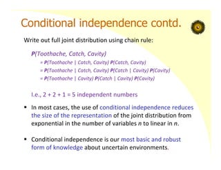
25. Conditional independence contd.
Write out full joint distribution using chain rule:
P(Toothache, Catch, Cavity)
= P(Toothache | Catch, Cavity) P(Catch, Cavity)
= P(Toothache | Catch, Cavity) P(Catch | Cavity) P(Cavity)
= P(Toothache | Cavity) P(Catch | Cavity) P(Cavity)
I.e., 2 + 2 + 1 = 5 independent numbers
 In most cases, the use of conditional independence reduces
the size of the representation of the joint distribution from
exponential in the number of variables n to linear in n.
 Conditional independence is our most basic and robust
form of knowledge about uncertain environments.

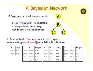
26. A Bayesian Network
A Bayesian network is made up of:
A P(A)
false 0.6
true 0.4
A
B
C D
A B P(B|A)
false false 0.01
false true 0.99
true false 0.7
true true 0.3
B C P(C|B)
false false 0.4
false true 0.6
true false 0.9
true true 0.1
B D P(D|B)
false false 0.02
false true 0.98
true false 0.05
true true 0.95
1. A Directed Acyclic Graph (DAG):
language for representing
(conditional) independences
2. A set of tables for each node in the graph,
representing (conditional) probability distributions

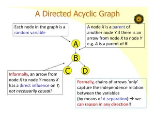
27. A Directed Acyclic Graph
A
B
C D
Each node in the graph is a
random variable
A node X is a parent of
another node Y if there is an
arrow from node X to node Y
e.g. A is a parent of B
Informally, an arrow from
node X to node Y means X
has a direct influence on Y;
not necessarily causal!
Formally, chains of arrows ‘only’
capture the independence relation
between the variables
(by means of d‐separation)  we
can reason in any direction!!

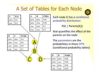
28. A Set of Tables for Each Node
Each node Xi has a conditional
probability distribution
P(Xi | Parents(Xi))
that quantifies the effect of the
parents on the node
The parameters are the
probabilities in these CPTs
(conditional probability tables)
A P(A)
false 0.6
true 0.4
A B P(B|A)
false false 0.01
false True 0.99
true false 0.7
true true 0.3
B C P(C|B)
false false 0.4
false true 0.6
true false 0.9
true true 0.1
B D P(D|B)
false false 0.02
false true 0.98
true false 0.05
true true 0.95
A
B
C D

29. A Set of Tables for Each Node
Conditional Probability
Distributions for C given B
If you have a Boolean variable with k Boolean parents, this table
has 2k+1 probabilities (but only 2k need to be stored)
B C P(C|B)
false false 0.4
false true 0.6
true false 0.9
true true 0.1
For a given combination of conditioning
values (for parents), the entries for
P(C=true | B) and P(C=false | B) must add
to 1, e.g.
P(C=true | B=false) + P(C=false |B=false)=1

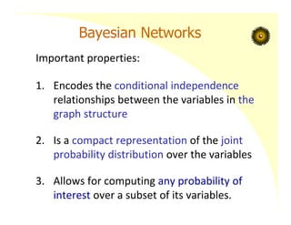
30. Bayesian Networks
Important properties:
1. Encodes the conditional independence
relationships between the variables in the
graph structure
2. Is a compact representation of the joint
probability distribution over the variables
3. Allows for computing any probability of
interest over a subset of its variables.

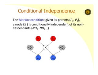
31. Conditional Independence
The Markov condition: given its parents (P1, P2),
a node (X ) is conditionally independent of its non‐
descendants (ND1, ND2,….)
X
P1 P2
C1 C2
ND2
ND1

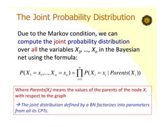
32. The Joint Probability Distribution
Due to the Markov condition, we can
compute the joint probability distribution
over all the variables X1, …, Xn in the Bayesian
net using the formula:






n
i
i
i
i
n
n X
Parents
x
X
P
x
X
x
X
P
1
1
1 ))
(
|
(
)
,...,
(
Where Parents(Xi) means the values of the parents of the node Xi
with respect to the graph
 The joint distribution defined by a BN factorizes into parameters
from all its CPTs.

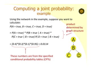
33. Computing a joint probability:
example
Using the network in the example, suppose you want to
calculate:
P(A = true, B = true, C = true, D = true)
= P(A = true) * P(B = true | A = true) *
P(C = true | B = true) P( D = true | B = true)
= (0.4)*(0.3)*(0.1)*(0.95) = 0.0114
A
B
C D
product
determined by
graph structure
These numbers are from the specified
conditional probability tables (CPTs)

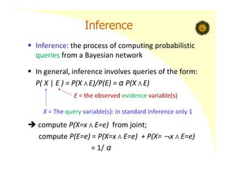
34. Inference
 Inference: the process of computing probabilistic
queries from a Bayesian network
 In general, inference involves queries of the form:
P( X | E ) = P(X ⋀ E)/P(E) = α P(X ⋀ E)
 compute P(X=x ⋀ E=e) from joint;
compute P(E=e) = P(X=x ⋀ E=e) + P(X= x ⋀ E=e)
= 1/ α
X = The query variable(s): in standard inference only 1
E = the observed evidence variable(s)

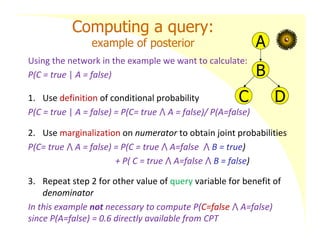
35. Computing a query:
example of posterior
Using the network in the example we want to calculate:
P(C = true | A = false)
1. Use definition of conditional probability
P(C = true | A = false) = P(C= true ⋀ A = false)/ P(A=false)
2. Use marginalization on numerator to obtain joint probabilities
P(C= true ⋀ A = false) = P(C = true ⋀ A=false ⋀ B = true)
+ P( C = true ⋀ A=false ⋀ B = false)
3. Repeat step 2 for other value of query variable for benefit of
denominator
In this example not necessary to compute P(C=false ⋀ A=false)
since P(A=false) = 0.6 directly available from CPT
A
B
C D

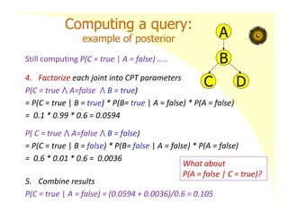
36. Computing a query:
example of posterior
Still computing P(C = true | A = false) …..
4. Factorize each joint into CPT parameters
P(C = true ⋀ A=false ⋀ B = true)
= P(C = true | B = true) * P(B= true | A = false) * P(A = false)
= 0.1 * 0.99 * 0.6 = 0.0594
P( C = true ⋀ A=false ⋀ B = false)
= P(C = true | B = false) * P(B= false | A = false) * P(A = false)
= 0.6 * 0.01 * 0.6 = 0.0036
5. Combine results
P(C = true | A = false) = (0.0594 + 0.0036)/0.6 = 0.105
A
B
C D
What about
P(A = false | C = true)?

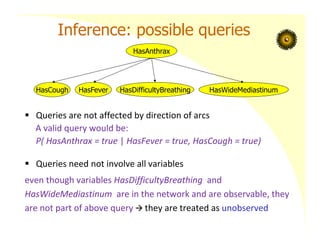
37. Inference: possible queries
 Queries are not affected by direction of arcs
A valid query would be:
P( HasAnthrax = true | HasFever = true, HasCough = true)
 Queries need not involve all variables
even though variables HasDifficultyBreathing and
HasWideMediastinum are in the network and are observable, they
are not part of above query  they are treated as unobserved
HasAnthrax
HasCough HasFever HasDifficultyBreathing HasWideMediastinum

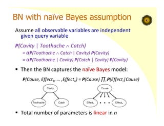
38. BN with naïve Bayes assumption
Assume all observable variables are independent
given query variable
P(Cavity | Toothache  Catch)
= αP(Toothache  Catch | Cavity) P(Cavity)
= αP(Toothache | Cavity) P(Catch | Cavity) P(Cavity)
 Then the BN captures the naïve Bayes model:
P(Cause, Effect1, … ,Effectn) = P(Cause) ∏i P(Effecti|Cause)
 Total number of parameters is linear in n

39. Complexity
 Exact inference is NP‐hard:
– Exact inference is feasible in small to medium‐
sized networks
– Exact inference in large, dense networks takes
a very long time
 Approximate inference techniques exist
– are much faster
– give pretty good results (but no guarantees)

40. How to build BNs
There are two options
(or combinations thereof):
 Handcrafting with the help of an expert in
the domain of application
 Machine learning it from data

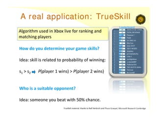
41. A real application: TrueSkill
Algorithm used in Xbox live for ranking and
matching players
How do you determine your game skills?
Idea: skill is related to probability of winning:
s1 > s2 P(player 1 wins) > P(player 2 wins)
Who is a suitable opponent?
Idea: someone you beat with 50% chance.
TrueSkill material: thanks to Ralf Herbrich and Thore Graepel, Microsoft Research Cambridge
Leaderboard

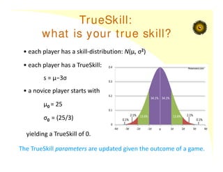
42. TrueSkill:
what is your true skill?
• each player has a skill‐distribution: N(μ, σ2)
• each player has a TrueSkill:
s = μ−3σ
• a novice player starts with
μ0 = 25
σ0 = (25/3)
yielding a TrueSkill of 0.
Moserware.com
The TrueSkill parameters are updated given the outcome of a game.

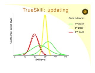
43. TrueSkill: updating
0 10 20 30 40 50
Skill-level
‘Confidence’
in
skill-level
1ste place
2de place
3rde place
Game outcome:

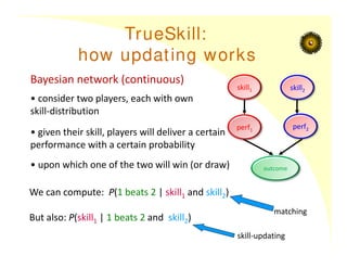
44. TrueSkill:
how updating works
outcome
perf1
perf2
skill1 skill2
Bayesian network (continuous)
• consider two players, each with own
skill‐distribution
• given their skill, players will deliver a certain
performance with a certain probability
• upon which one of the two will win (or draw)
We can compute: P(1 beats 2 | skill1 and skill2)
But also: P(skill1 | 1 beats 2 and skill2)
matching
skill‐updating

45. Does it work? An experiment…
Data Sets: Halo 2 Beta,
Halo 3 Public Beta
3 game modes: ‘Free-for-All’
Two Teams
1-on-1
Thousands of players, 10-thousands of
outcomes

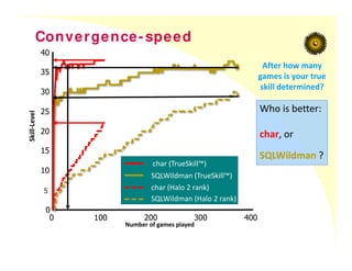
46. 0
10
15
20
25
30
35
40
Skill‐Level
0 100 200 300 400
Number of games played
char (Halo 2 rank)
SQLWildman (Halo 2 rank)
char (TrueSkill™)
SQLWildman (TrueSkill™)
Convergence-speed
After how many
games is your true
skill determined?
Who is better:
char, or
SQLWildman ?
5

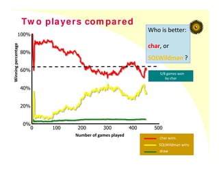
47. 0 100 200 300 400 500
0%
20%
40%
60%
80%
100%
Number of games played
Winning
percentage
5/8 games won
by char
SQLWildman wins
char wins
draw
Tw o players com pared
Who is better:
char, or
SQLWildman ?

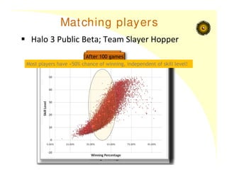
48. Matching players
 Halo 3 Public Beta; Team Slayer Hopper
After 1 game
…10 games
… 30 games
After 100 games
Most players have ≈50% chance of winning, independent of skill level!
Most players have ≈50% chance of winning, independent of skill level!

49. Applications of BN
Also: Bayesian medical kiosk (http://vimeo.com/64474130)