Ai Uncertainty reasoning

1. Artificial Intelligence
Chapter 13: Quantifying Uncertainty

3. JK

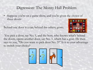
4. Digression: The Monty Hall Problem
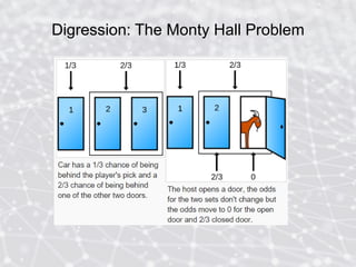
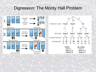
• Suppose you're on a game show, and you're given the choice of
three doors:
Behind one door is a car; behind the others, goats.
You pick a door, say No. 1, and the host, who knows what's behind
the doors, opens another door, say No. 3, which has a goat. He then
says to you, "Do you want to pick door No. 2?" Is it to your advantage
to switch your choice?

5. Digression: The Monty Hall Problem

6. Digression: The Monty Hall Problem

7. Uncertainty
• Agents need to handle uncertainty, whether due to partial
observability, non-determinism, or a combination of the two.
• In Chapter 4, we encountered problem-solving agents designed
to handle uncertainty by monitoring a belief-state – a
representation of the set of all possible world states in which
the agent might find itself (e.g. AND-OR graphs).
• The agent generated a contingency plan that handles every
possible eventuality that its sensors report during execution.

8. Uncertainty
• Despite its many virtues, however, this approach has many
significant drawbacks:
(*) With partial information, an agent must consider every
possible eventuality, no matter how unlikely. This leads to
impossibly large and complex belief-state representations.
(*) A correct contingency plan that handles every possible
outcome can grow arbitrarily large and must consider arbitrarily
unlikely contingencies.
(*) Sometimes there is, in fact, no plan that is guaranteed to
achieve a stated goal – yet the agent must act. It must have some
way to compare the merits of plans that are not guaranteed.

9. Uncertainty
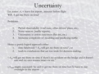
Let action At = leave for airport t minutes before flight
Will At get me there on time?
Problems:
1. Partial observability (road state, other drivers' plans, etc.)
2. Noisy sensors (traffic reports)
3. Uncertainty in action outcomes (flat tire, etc.)
4. Immense complexity of modeling and predicting traffic
Hence a purely logical approach either
1. risks falsehood: “A25 will get me there on time”, or
2. leads to conclusions that are too weak for decision making:
“A25 will get me there on time if there's no accident on the bridge and it doesn't
rain and my tires remain intact etc etc.”
(A1440 might reasonably be said to get me there on time but I'd have to stay
overnight in the airport …)

10. Uncertainty
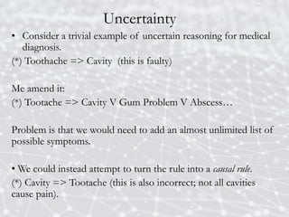
• Consider a trivial example of uncertain reasoning for medical
diagnosis.
(*) Toothache => Cavity (this is faulty)
Me amend it:
(*) Tootache => Cavity V Gum Problem V Abscess…
Problem is that we would need to add an almost unlimited list of
possible symptoms.
• We could instead attempt to turn the rule into a causal rule.
(*) Cavity => Tootache (this is also incorrect; not all cavities
cause pain).

11. Uncertainty
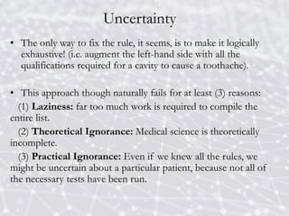
• The only way to fix the rule, it seems, is to make it logically
exhaustive! (i.e. augment the left-hand side with all the
qualifications required for a cavity to cause a toothache).
• This approach though naturally fails for at least (3) reasons:
(1) Laziness: far too much work is required to compile the
entire list.
(2) Theoretical Ignorance: Medical science is theoretically
incomplete.
(3) Practical Ignorance: Even if we knew all the rules, we
might be uncertain about a particular patient, because not all of
the necessary tests have been run.

12. Uncertainty
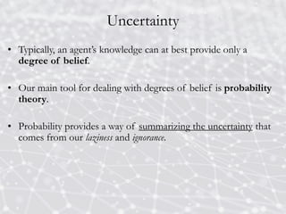
• Typically, an agent’s knowledge can at best provide only a
degree of belief.
• Our main tool for dealing with degrees of belief is probability
theory.
• Probability provides a way of summarizing the uncertainty that
comes from our laziness and ignorance.

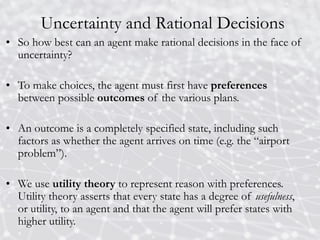
13. Uncertainty and Rational Decisions
• So how best can an agent make rational decisions in the face of
uncertainty?
• To make choices, the agent must first have preferences
between possible outcomes of the various plans.
• An outcome is a completely specified state, including such
factors as whether the agent arrives on time (e.g. the “airport
problem”).
• We use utility theory to represent reason with preferences.
Utility theory asserts that every state has a degree of usefulness,
or utility, to an agent and that the agent will prefer states with
higher utility.

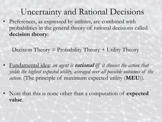
14. Uncertainty and Rational Decisions
• Preferences, as expressed by utilities, are combined with
probabilities in the general theory of rational decisions called
decision theory:
Decision Theory = Probability Theory + Utility Theory
• Fundamental idea: an agent is rational iff it chooses the action that
yields the highest expected utility, averaged over all possible outcomes of the
action. (The principle of maximum expected utility (MEU)).
• Note that this is none other than a computation of expected
value.

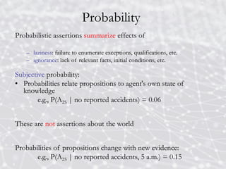
15. Probability
Probabilistic assertions summarize effects of
– laziness: failure to enumerate exceptions, qualifications, etc.
– ignorance: lack of relevant facts, initial conditions, etc.
Subjective probability:
• Probabilities relate propositions to agent's own state of
knowledge
e.g., P(A25 | no reported accidents) = 0.06
These are not assertions about the world
Probabilities of propositions change with new evidence:
e.g., P(A25 | no reported accidents, 5 a.m.) = 0.15

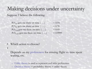
16. Making decisions under uncertainty
Suppose I believe the following:
P(A25 gets me there on time | …) = 0.04
P(A90 gets me there on time | …) = 0.70
P(A120 gets me there on time | …) = 0.95
P(A1440 gets me there on time | …) = 0.9999
• Which action to choose?
•
Depends on my preferences for missing flight vs. time spent
waiting, etc.
– Utility theory is used to represent and infer preferences
– Decision theory = probability theory + utility theory

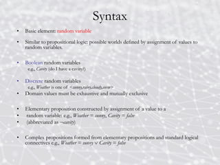
17. Syntax
• Basic element: random variable
• Similar to propositional logic: possible worlds defined by assignment of values to
random variables.
• Boolean random variables
e.g., Cavity (do I have a cavity?)
• Discrete random variables
e.g., Weather is one of <sunny,rainy,cloudy,snow>
• Domain values must be exhaustive and mutually exclusive
• Elementary proposition constructed by assignment of a value to a
• random variable: e.g., Weather = sunny, Cavity = false
• (abbreviated as cavity)
• Complex propositions formed from elementary propositions and standard logical
connectives e.g., Weather = sunny  Cavity = false

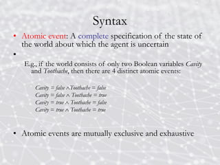
18. Syntax
• Atomic event: A complete specification of the state of
the world about which the agent is uncertain
•
E.g., if the world consists of only two Boolean variables Cavity
and Toothache, then there are 4 distinct atomic events:
Cavity = false Toothache = false
Cavity = false  Toothache = true
Cavity = true  Toothache = false
Cavity = true  Toothache = true
• Atomic events are mutually exclusive and exhaustive

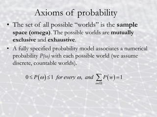
19. Axioms of probability
• The set of all possible “worlds” is the sample
space (omega). The possible worlds are mutually
exclusive and exhaustive.
• A fully specified probability model associates a numerical
probability P(ω) with each possible world (we assume
discrete, countable worlds).
   
0 1 , 1
P for every and P w

 

  


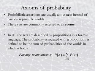
20. Axioms of probability
• Probabilistic assertions are usually about sets instead of
particular possible worlds.
• These sets are commonly referred to as events.
• In AI, the sets are described by propositions in a formal
language. The probability associated with a proposition is
defined to be the sum of probabilities of the worlds in
which it holds:
   
,
For any proposition P P
 
  

 

21. Axioms of probability
• Probabilistic assertions are usually about sets instead of
particular possible worlds.
• These sets are commonly referred to as events.
• In AI, the sets are described by propositions in a formal
language. The probability associated with a proposition is
defined to be the sum of probabilities of the worlds in
which it holds:
   
,
For any proposition P P
 
  

 

22. Axioms of probability
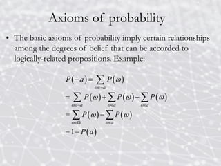
• The basic axioms of probability imply certain relationships
among the degrees of belief that can be accorded to
logically-related propositions. Example:
   
     
   
 
1
a
a a a
a
P a P
P P P
P P
P a

  
 

  
 

  
 
 
  
 
 

  
 

23. Axioms of probability
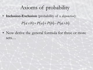
• Inclusion-Exclusion (probability of a disjunction):
• Now derive the general formula for three or more
sets…
       
P a b P a P b P a b
    

24. Axioms of probability
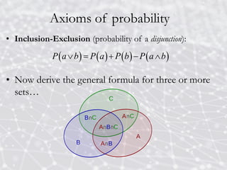
• Inclusion-Exclusion (probability of a disjunction):
• Now derive the general formula for three or more
sets…
       
P a b P a P b P a b
    

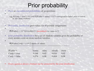
25. Prior probability
• Prior or unconditional probabilities of propositions
•
e.g., P(Cavity = true) = 0.1 and P(Weather = sunny) = 0.72 correspond to belief prior to arrival
of any (new) evidence
• Probability distribution gives values for all possible assignments:
•
P(Weather) = <0.72,0.1,0.08,0.1> (normalized, i.e., sums to 1)
• Joint probability distribution for a set of random variables gives the probability of
every atomic event on those random variables
•
P(Weather,Cavity) = a 4 × 2 matrix of values:
Weather = sunny rainy cloudy snow
Cavity = true 0.144 0.02 0.016 0.02
Cavity = false 0.576 0.08 0.064 0.08
• Every question about a domain can be answered by the joint distribution

26. Conditional probability
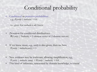
• Conditional or posterior probabilities
e.g., P(cavity | toothache) = 0.8
i.e., given that toothache is all I know
• (Notation for conditional distributions:
P(Cavity | Toothache) = 2-element vector of 2-element vectors)
• If we know more, e.g., cavity is also given, then we have
P(cavity | toothache,cavity) = 1
• New evidence may be irrelevant, allowing simplification, e.g.,
P(cavity | toothache, sunny) = P(cavity | toothache) = 0.8
• This kind of inference, sanctioned by domain knowledge, is crucial

27. Conditional probability
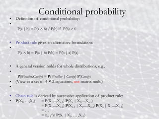
• Definition of conditional probability:
•
P(a | b) = P(a  b) / P(b) if P(b) > 0
• Product rule gives an alternative formulation:
•
P(a  b) = P(a | b) P(b) = P(b | a) P(a)
• A general version holds for whole distributions, e.g.,
•
P(Weather,Cavity) = P(Weather | Cavity) P(Cavity)
• (View as a set of 4 × 2 equations, not matrix mult.)
•
• Chain rule is derived by successive application of product rule:
• P(X1, …,Xn) = P(X1,...,Xn-1) P(Xn | X1,...,Xn-1)
= P(X1,...,Xn-2) P(Xn-1 | X1,...,Xn-2) P(Xn | X1,...,Xn-1)
= …
= πi= 1^n P(Xi | X1, … ,Xi-1)

28. Bayesian and Frequentist Probability
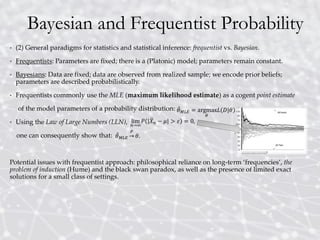
• (2) General paradigms for statistics and statistical inference: frequentist vs. Bayesian.
• Frequentists: Parameters are fixed; there is a (Platonic) model; parameters remain constant.
• Bayesians: Data are fixed; data are observed from realized sample; we encode prior beliefs;
parameters are described probabilistically.
• Frequentists commonly use the MLE (maximum likelihood estimate) as a cogent point estimate
of the model parameters of a probability distribution:
• Using the Law of Large Numbers (LLN),
one can consequently show that:
Potential issues with frequentist approach: philosophical reliance on long-term ‘frequencies’, the
problem of induction (Hume) and the black swan paradox, as well as the presence of limited exact
solutions for a small class of settings.

29. Bayesian and Frequentist Probability
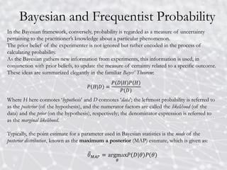
In the Bayesian framework, conversely, probability is regarded as a measure of uncertainty
pertaining to the practitioner’s knowledge about a particular phenomenon.
The prior belief of the experimenter is not ignored but rather encoded in the process of
calculating probability.
As the Bayesian gathers new information from experiments, this information is used, in
conjunction with prior beliefs, to update the measure of certainty related to a specific outcome.
These ideas are summarized elegantly in the familiar Bayes’ Theorem:
Where H here connotes ‘hypothesis’ and D connotes ‘data’; the leftmost probability is referred to
as the posterior (of the hypothesis), and the numerator factors are called the likelihood (of the
data) and the prior (on the hypothesis), respectively; the denominator expression is referred to
as the marginal likelihood.
Typically, the point estimate for a parameter used in Bayesian statistics is the mode of the
posterior distribution, known as the maximum a posterior (MAP) estimate, which is given as:

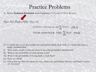
30. Practice Problems
(1) Derive Inclusion-Exclusion from Equations (13.1) and (13.2) in the text.
(2) Consider the set of all possible five-card poker hands dealt fairly (i.e. randomly) from a
single, standard deck.
(i) How many atomic events are there in the joint probability distribution?
(ii) What is the probability of each atomic event?
(iii) What is the probability of being dealt a royal flush?
(iv) Four of a kind?
(v) Given that my first two cards are aces, what is the probability that my total hand consists
of four aces?
(13.1)
(13.2)

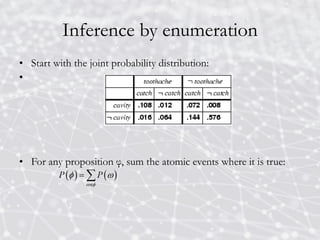
31. Inference by enumeration
• Start with the joint probability distribution:
•
• For any proposition φ, sum the atomic events where it is true:

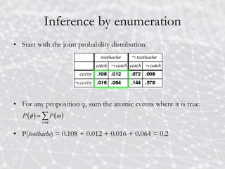
32. Inference by enumeration
• Start with the joint probability distribution:
• For any proposition φ, sum the atomic events where it is true:
• P(toothache) = 0.108 + 0.012 + 0.016 + 0.064 = 0.2

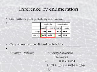
33. Inference by enumeration
• Start with the joint probability distribution:
•
• Can also compute conditional probabilities:
•
P(cavity | toothache) = P(cavity  toothache)
P(toothache)
= 0.016+0.064
0.108 + 0.012 + 0.016 + 0.064
= 0.4

34. Normalization
• Denominator can be viewed as a normalization constant α
•
P(Cavity | toothache) = α, P(Cavity,toothache)
= α, [P(Cavity,toothache,catch) + P(Cavity,toothache, catch)]
= α, [<0.108,0.016> + <0.012,0.064>]
= α, <0.12,0.08> = <0.6,0.4>
General idea: compute distribution on query variable by fixing evidence variables
and summing over hidden variables

35. Inference by enumeration
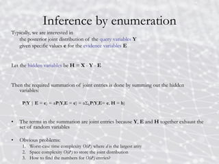
Typically, we are interested in
the posterior joint distribution of the query variables Y
given specific values e for the evidence variables E
Let the hidden variables be H = X - Y - E
Then the required summation of joint entries is done by summing out the hidden
variables:
P(Y | E = e) = αP(Y,E = e) = αΣhP(Y,E= e, H = h)
• The terms in the summation are joint entries because Y, E and H together exhaust the
set of random variables
• Obvious problems:
1. Worst-case time complexity O(dn) where d is the largest arity
2. Space complexity O(dn) to store the joint distribution
3. How to find the numbers for O(dn) entries?

36. Independence
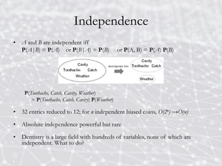
• A and B are independent iff
P(A|B) = P(A) or P(B|A) = P(B) or P(A, B) = P(A) P(B)
P(Toothache, Catch, Cavity, Weather)
= P(Toothache, Catch, Cavity) P(Weather)
• 32 entries reduced to 12; for n independent biased coins, O(2n) →O(n)
• Absolute independence powerful but rare
• Dentistry is a large field with hundreds of variables, none of which are
independent. What to do?

37. Conditional independence
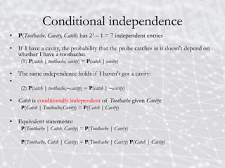
• P(Toothache, Cavity, Catch) has 23 – 1 = 7 independent entries
• If I have a cavity, the probability that the probe catches in it doesn't depend on
whether I have a toothache:
(1) P(catch | toothache, cavity) = P(catch | cavity)
• The same independence holds if I haven't got a cavity:
•
(2) P(catch | toothache,cavity) = P(catch | cavity)
• Catch is conditionally independent of Toothache given Cavity:
P(Catch | Toothache,Cavity) = P(Catch | Cavity)
• Equivalent statements:
P(Toothache | Catch, Cavity) = P(Toothache | Cavity)
P(Toothache, Catch | Cavity) = P(Toothache | Cavity) P(Catch | Cavity)

38. Conditional independence
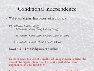
• Write out full joint distribution using chain rule:
•
P(Toothache, Catch, Cavity)
= P(Toothache | Catch, Cavity) P(Catch, Cavity)
= P(Toothache | Catch, Cavity) P(Catch | Cavity) P(Cavity)
= P(Toothache | Cavity) P(Catch | Cavity) P(Cavity)
I.e., 2 + 2 + 1 = 5 independent numbers
• In most cases, the use of conditional independence reduces the
size of the representation of the joint distribution from
exponential in n to linear in n.

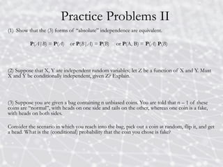
39. Practice Problems II
(1) Show that the (3) forms of “absolute” independence are equivalent.
P(A|B) = P(A) or P(B|A) = P(B) or P(A, B) = P(A) P(B)
(2) Suppose that X, Y are independent random variables; let Z be a function of X and Y. Must
X and Y be conditionally independent, given Z? Explain.
(3) Suppose you are given a bag containing n unbiased coins. You are told that n – 1 of these
coins are “normal”, with heads on one side and tails on the other, whereas one coin is a fake,
with heads on both sides.
Consider the scenario in which you reach into the bag, pick out a coin at random, flip it, and get
a head. What is the (conditional) probability that the coin you chose is fake?

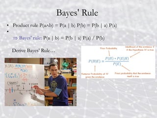
40. Bayes' Rule
• Product rule P(ab) = P(a | b) P(b) = P(b | a) P(a)
•
 Bayes' rule: P(a | b) = P(b | a) P(a) / P(b)
Derive Bayes’ Rule…

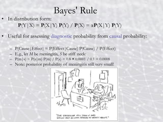
41. Bayes' Rule
• In distribution form:
P(Y|X) = P(X|Y) P(Y) / P(X) = αP(X|Y) P(Y)
• Useful for assessing diagnostic probability from causal probability:
– P(Cause|Effect) = P(Effect|Cause) P(Cause) / P(Effect)
– E.g., let M be meningitis, S be stiff neck:
– P(m|s) = P(s|m) P(m) / P(s) = 0.8 × 0.0001 / 0.1 = 0.0008
– Note: posterior probability of meningitis still very small!

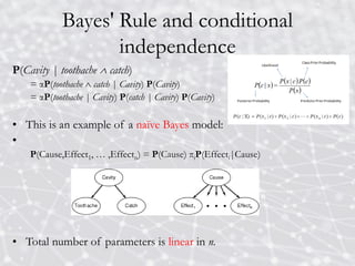
42. Bayes' Rule and conditional
independence
P(Cavity | toothache  catch)
= αP(toothache  catch | Cavity) P(Cavity)
= αP(toothache | Cavity) P(catch | Cavity) P(Cavity)
• This is an example of a naïve Bayes model:
•
P(Cause,Effect1, … ,Effectn) = P(Cause) πiP(Effecti|Cause)
• Total number of parameters is linear in n.

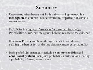
43. Summary
• Uncertainty arises because of both laziness and ignorance. It is
inescapable in complex, nondeterministic, or partially observable
environments.
• Probability is a rigorous formalism for uncertain knowledge.
Probabilities summarize the agent’s believes relative to the evidence.
• Decision Theory combines the agent’s beliefs and desires,
defining the best action as the one that maximizes expected utility.
• Basic probability statements include priors probabilities and
conditional probabilities. Joint probabilities distributions specifiy
a probability of every atomic event.

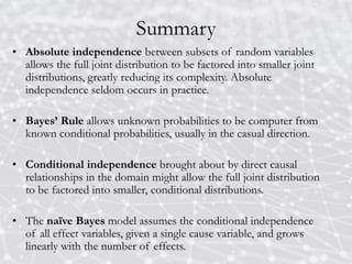
44. Summary
• Absolute independence between subsets of random variables
allows the full joint distribution to be factored into smaller joint
distributions, greatly reducing its complexity. Absolute
independence seldom occurs in practice.
• Bayes’ Rule allows unknown probabilities to be computer from
known conditional probabilities, usually in the casual direction.
• Conditional independence brought about by direct causal
relationships in the domain might allow the full joint distribution
to be factored into smaller, conditional distributions.
• The naïve Bayes model assumes the conditional independence
of all effect variables, given a single cause variable, and grows
linearly with the number of effects.