Physics Of The Large And The Small Tasi 2009 Proceedings Of The 2009 Theoretical Advanced Study Institute In Elementary Particle Physics Csaba Csaki
Physics Of The Large And The Small Tasi 2009 Proceedings Of The 2009 Theoretical Advanced Study Institute In Elementary Particle Physics Csaba Csaki
Physics Of The Large And The Small Tasi 2009 Proceedings Of The 2009 Theoretical Advanced Study Institute In Elementary Particle Physics Csaba Csaki


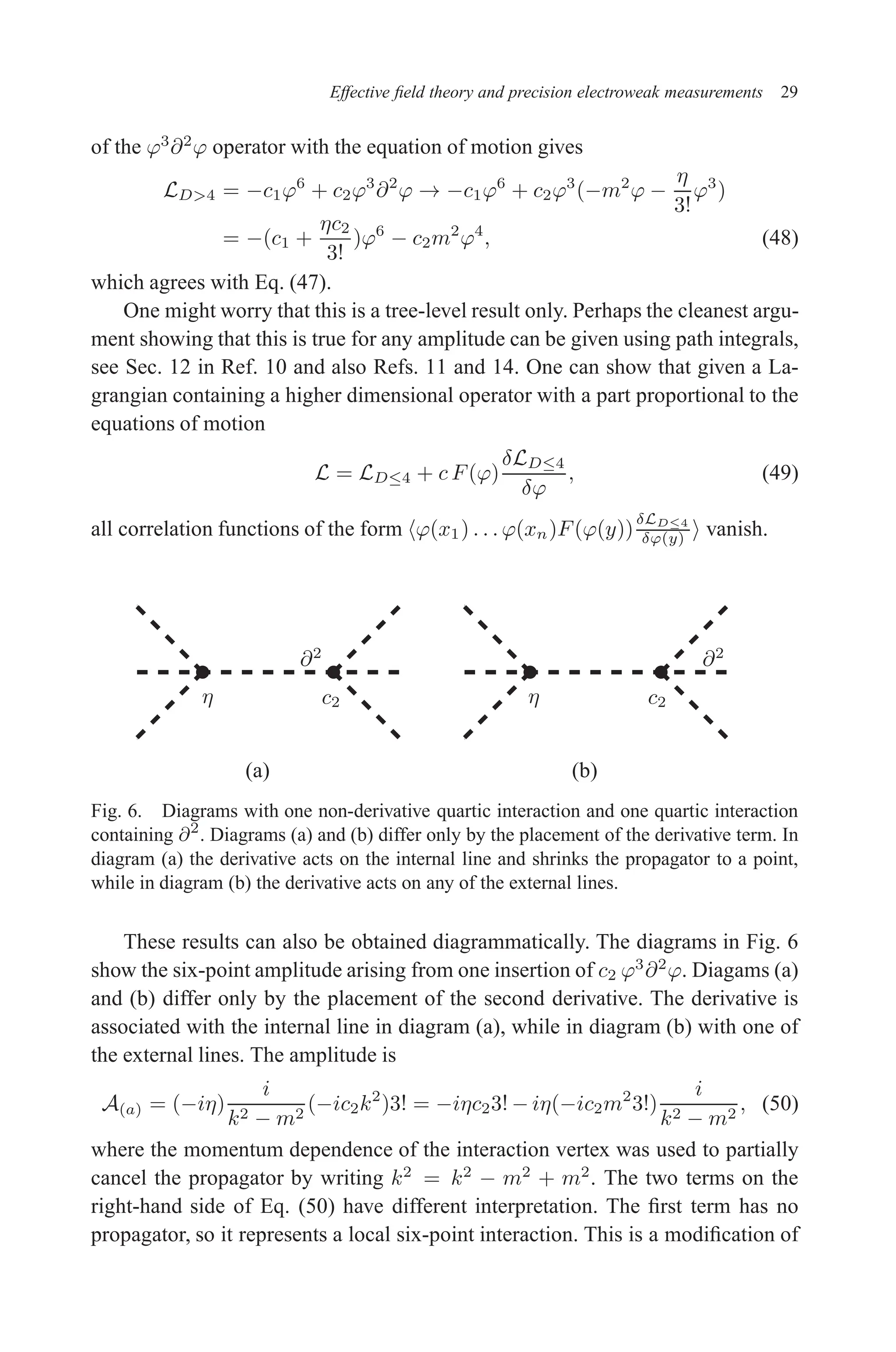
![December 22, 2010 9:24 WSPC - Proceedings Trim Size: 9in x 6in tasi2009
10 W. Skiba
When constructing an EFT one needs to be able to formally predict the mag-
nitudes of different Oi terms in the effective Lagrangian. This is referred to as
power counting the terms in the Lagrangian and it allows one to predict how dif-
ferent terms scale with energy. In the simple EFTs discussed here, power counting
is the same as dimensional analysis using the natural ~ = c = 1 units, in which
[mass] = [length]−1
. From now on, dimensions will be expressed in the units
of [mass], so that energy has dimension 1, while length has dimension −1. The
Lagrangian density has dimension 4 since
R
L d4
x must be dimensionless.
The dimensions of fields are determined from their kinetic energies because
in weakly interacting theories these terms always dominate. The kinetic energy
term for a scalar field, ∂µφ ∂µ
φ, implies that φ has dimension 1, while that of a
fermion, i ψ /
∂ ψ, implies that ψ has dimension 3
2 in 4 space-time dimensions.
A Yukawa theory consisting of a massless fermion interacting with with two
real scalar fields: a light one and a heavy one will serve as our working example.
The Lagrangian of the high-energy theory is taken to be
L = iψ /
∂ ψ +
1
2
(∂µΦ)2
−
M2
2
Φ2
+
1
2
(∂µϕ)2
−
m2
2
ϕ2
− λ ψψΦ − η ψψϕ. (3)
Let us assume that M m. As this is a toy example, we do not worry whether
it is natural to have a hierarchy between m and M. The Yukawa couplings are
denoted as λ and η. We neglect the potential for Φ and ϕ as it is unimportant for
now.
As our first example of an EFT, we will consider tree-level effects. We want
to find an effective theory with only the light fields present: the fermion ψ and
scalar ϕ. The interactions generated by the exchanges of the heavy field Ψ will be
mocked up by new interactions involving the light fields.
We want to examine the ψψ → ψψ scattering process to order λ2
in the
coupling constants, that is to the zeroth order in η, and keep terms to the second
order in the external momenta.
−
Φ
ψ
ψ ψ
ψ
Φ
1
2
3
4
1
2
3
4
Fig. 1. Tree-level diagrams proportional to λ2
that contribute to ψψ → ψψ scattering.](https://image.slidesharecdn.com/2325148-250520022801-8a7295d5/75/Physics-Of-The-Large-And-The-Small-Tasi-2009-Proceedings-Of-The-2009-Theoretical-Advanced-Study-Institute-In-Elementary-Particle-Physics-Csaba-Csaki-25-2048.jpg)
![December 22, 2010 9:24 WSPC - Proceedings Trim Size: 9in x 6in tasi2009
14 W. Skiba
the two-derivative term is not suppressed at all. Since the same argument holds
for terms with more and more derivatives, all terms would contribute exactly the
same and the momentum expansion would be pointless. This is, for example, how
hard momentum cut off and Pauli-Villars regulators behave. Such regulators do
their job, but they needlessly complicate power counting. From now on, we will
only be using dimensional regularization.
To calculate the RG running of the coefficient c, we need to obtain the relevant
Z factors. First, we need the fermion self energy diagram
p p + k
k
= (−iη)2
Z
dd
k
(2π)d
i(/
k + /
p)
(k + p)2
i
k2 − m2
= η2
Z
dd
l
(2π)d
Z 1
0
dx
/
l + (1 − x)/
p
[l2 − ∆2]2
=
iη2
(4π)2
1
ǫ
Z 1
0
dx(1 − x)/
p
+ finite
=
iη2
/
p
2(4π)2
1
ǫ
+ finite, (11)
where we used Feynman parameters to combine the denominators and shifted the
loop momentum l = k + xp. We then used the standard result for loop integrals
and expanded d = 4 − 2ǫ. Only the 1
ǫ pole is kept as the finite term does not enter
the RG calculation.
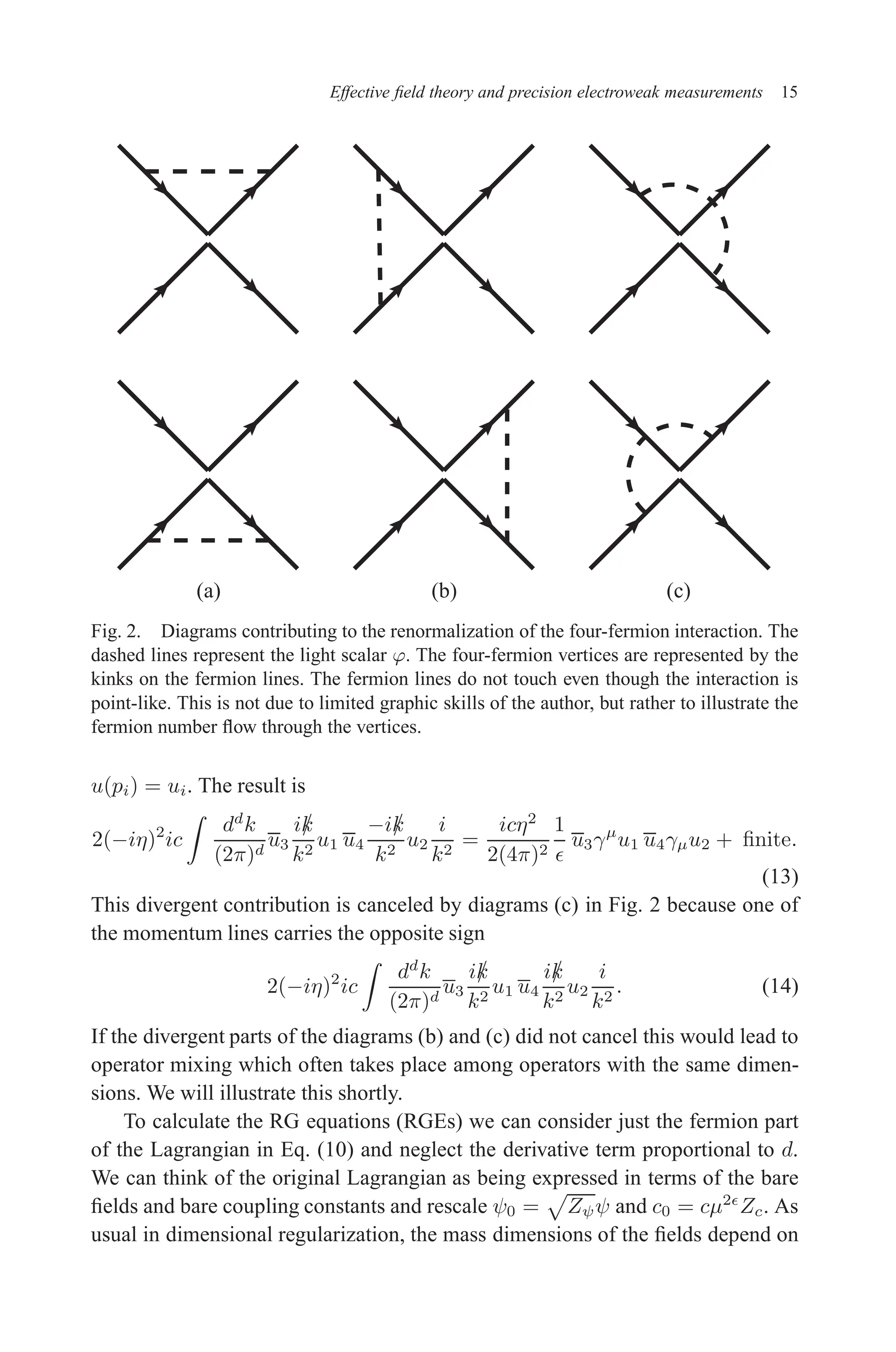
The second part of the calculation involves computing loop corrections to the
four-fermion vertex. There are six diagrams with a scalar exchange because there
are six different pairings of the external lines. The diagrams are depicted in Fig. 2
and there are two diagrams in each of the three topologies. All of these diagrams
are logarithmically divergent in the UV, so we can neglect the external momenta
and masses if we are interested in the divergent parts. The divergent terms must be
local and therefore be analytic in the external momenta. Extracting positive pow-
ers of momenta from a diagram reduces its degree of divergence which is apparent
from dimensional analysis. Diagrams (a) in Fig. 2 are the most straightforward to
deal with and the divergent part is easy to extract
2(−iη)2
ic
Z
dd
k
(2π)d
i/
k
k2
i/
k
k2
i
k2
= −2cη2
Z
dd
k
(2π)d
1
k4
= −
2icη2
(4π)2
1
ǫ
+ finite.
(12)
We did not mention the cross diagrams here, denoted {3 ↔ 4} in the previous
section, since they go along for the ride, but they participate in every step. Dia-
grams (b) in Fig. 2 require more care as the loop integral involves two different
fermion lines. To keep track of this we indicate the external spinors and abbreviate](https://image.slidesharecdn.com/2325148-250520022801-8a7295d5/75/Physics-Of-The-Large-And-The-Small-Tasi-2009-Proceedings-Of-The-2009-Theoretical-Advanced-Study-Institute-In-Elementary-Particle-Physics-Csaba-Csaki-29-2048.jpg)
![December 22, 2010 9:24 WSPC - Proceedings Trim Size: 9in x 6in tasi2009
16 W. Skiba
the dimension of space-time. In d = 4 − 2ǫ, the fermion dimension is [ψ] = 3
2 − ǫ
and [L] = 4 − 2ǫ. We explicitly compensate for this change from the usual 4
space-time dimensions by including the factor µ2ǫ
in the interaction term. This
way, the coupling c does not alter its dimension when d = 4−2ǫ. The Lagrangian
is then
L = iψ0 /
∂ ψ0 +
c0
2
ψ0ψ0 ψ0ψ0 = iZψψ /
∂ ψ +
c
2
ZcZ2
ψµ2ǫ
ψψ ψψ
= iψ/
∂ψ + µ2ǫ c
2
ψψ ψψ + i(Zψ − 1)ψ/
∂ψ + µ2ǫ c
2
(ZcZ2
ψ − 1)ψψ ψψ, (15)
where in the last line we separated the counterterms. We can read off the coun-
terterms from Eqs. (11) and (12) by insisting that the counterterms cancel the
divergences we calculated previously.
Zψ − 1 = −
η2
2(4π)2
1
ǫ
and c(ZcZ2
ψ − 1) =
2cη2
(4π)2
1
ǫ
, (16)
where we used the minimal subtraction (MS) prescription and hence retained only
the 1
ǫ poles. Comparing the two equations in (16), we obtain Zc = 1 + 3η2
(4π)2
1
ǫ .
The standard way of computing RGEs is to use the fact that the bare quantities
do not depend on the renormalization scale
0 = µ
d
dµ
c0 = µ
d
dµ
(cµ2ǫ
Zc) = βcµ2ǫ
Zc + 2ǫcµ2ǫ
Zc + cµ2ǫ
µ
d
dµ
Zc, (17)
where βc ≡ µ dc
dµ. We have µ d
dµ Zc = 3
(4π)2 2ηβη
1
ǫ . Just like we had to compensate
for the dimension of c, the renormalized coupling η needs an extra factor of µǫ
to
remain dimensionless in the space-time where d = 4 − 2ǫ. Repeating the same
manipulations we used in Eq. (17), we obtain βη = −ǫη − η
d log Zη
d log µ . Keeping the
derivative of Zη would give us a term that is of higher order in η as for any Z
factor the scale dependence comes from the couplings. Thus, we keep only the
first term, βη = −ǫη, and get µ d
dµ Zc = − 6η2
(4π)2 . Finally,
βc =
6η2
(4π)2
c. (18)
We can now complete our task and compute the low-energy coupling, and thus
the scattering amplitude, to the leading log order
c(m) = c(M) −
6η2
(4π)2
c log
M
m
=
λ2
M2
1 −
6η2
(4π)2
log
M
m
. (19)
Of course, at this point it requires little extra work to re-sum the logarithms by
solving the RGEs. First, one needs to solve for the running of η. We will not](https://image.slidesharecdn.com/2325148-250520022801-8a7295d5/75/Physics-Of-The-Large-And-The-Small-Tasi-2009-Proceedings-Of-The-2009-Theoretical-Advanced-Study-Institute-In-Elementary-Particle-Physics-Csaba-Csaki-31-2048.jpg)
![December 22, 2010 9:24 WSPC - Proceedings Trim Size: 9in x 6in tasi2009
Effective field theory and precision electroweak measurements 19
and that our effective theory is instead
Lp0,V = iψ /
∂ ψ +
cV
2
ψγµ
ψ ψγµψ +
1
2
(∂µϕ)2
−
m2
2
ϕ2
− η ψψϕ. (22)
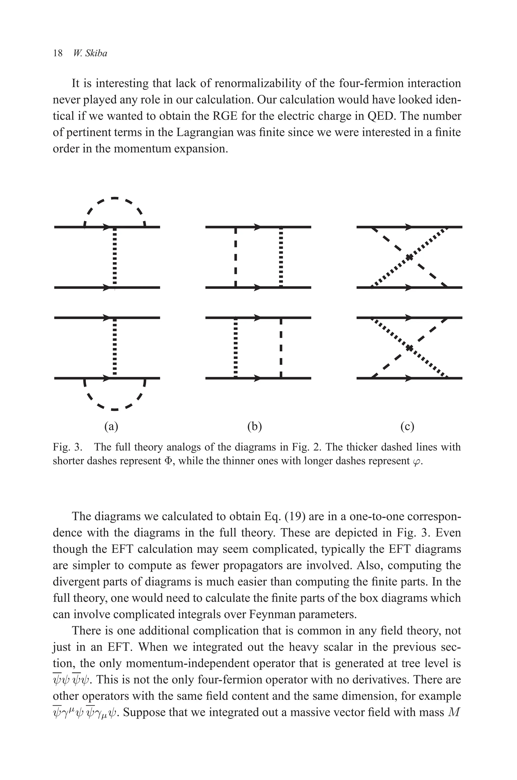
We could ask the same question about low-energy scattering in this theory, that
is ask about the RG evolution of the coefficient cV . The contributions from the
ϕ exchanges are identical to those depicted in Fig. 2. The only difference is that
the four-fermion vertex contains the γµ
matrices. Diagrams (a) give a divergent
contribution to the ψγµ
ψ ψγµψ operator. However, the sum of the divergent parts
of diagrams (b) and (c) is not proportional to the original operator, but instead pro-
portional to ψσµν
ψ ψσµν ψ, where σµν
= i
2 [γµ
, γν
]. This means that under RG
evolution these two operators mix. The two operators have the same dimensions,
field content, and symmetry properties thus loop corrections can turn one operator
into another.
To put it differently, it is not consistent to just keep a single four-fermion
operator in the effective Lagrangian in Eq. (22) at one loop. The theory needs to
be supplemented since there needs to be an additional counterterm to absorb the
divergence. At one loop it is enough to consider
Lp0,V T = iψ /
∂ ψ +
cV
2
ψγµ
ψ ψγµψ +
cT
2
ψσµν
ψ ψσµν ψ
+
1
2
(∂µϕ)2
−
m2
2
ϕ2
− η ψψϕ, (23)
but one expects that at higher loop orders all four-fermion operators are needed.
Since we assumed that the operator proportional to cV was generated by a heavy
vector field at tree level, we know that in our effective theory cT (µ = M) = 0
and cV (µ = M) 6= 0. At low energies, both coefficients will be nonzero.
We do not want to provide the calculation of the beta functions for the coef-
ficients cV and cT in great detail. This calculation is completely analogous to the
one for βc. The vector operator induces divergent contributions to itself and to the
tensor operator, while the tensor operator only generates a divergent contribution
for the vector operator. The coefficients of the two counterterms are
cV (ZV Z2
ψ − 1) =
η2
(4π)2
(−cV + 6cT )
1
ǫ
, (24)
cT (ZT Z2
ψ − 1) =
η2
(4π)2
cV
1
ǫ
, (25)
where we introduced separate Z factors for each operator since each requires a
counterterm. These Z factors imply that the beta functions are
βcV = 12 cT
η2
(4π)2
and βcT = 2 (cT + cV )
η2
(4π)2
. (26)](https://image.slidesharecdn.com/2325148-250520022801-8a7295d5/75/Physics-Of-The-Large-And-The-Small-Tasi-2009-Proceedings-Of-The-2009-Theoretical-Advanced-Study-Institute-In-Elementary-Particle-Physics-Csaba-Csaki-34-2048.jpg)
![December 22, 2010 9:24 WSPC - Proceedings Trim Size: 9in x 6in tasi2009
26 W. Skiba
are no tree-level diagrams involving fermions ψ in the internal lines only. We are
going to examine diagrams with two scalars and four scalars for illustration pur-
poses. The diagrams resemble those of the Coleman-Weinberg effective potential
calculation, but we do not necessarily neglect external momenta. The momentum
dependence could be of interest. The two point function gives
= (−1)(−iηµǫ
)2
Z
dd
k
(2π)d
i2
Tr[(/
k + /
p + M)(/
k + M)]
[(k + p)2 − M2](k2 − M2)
= −
4iη2
(4π)2
(
3
ǫ
+ 1 + 3 log(
µ2
M2
))(M2
−
p2
6
)
+
p2
2
−
p4
20M2
+ . . .
, (43)
where we truncated the momentum expansion at order p4
. The four-point ampli-
tude, to the lowest order in momentum is
= −
8iη4
(4π)2
3(
1
ǫ
+ log(
µ2
M2
)) − 8 + . . .
. (44)
There are no logarithms involving m2
or p2
in Eqs. (43) and (44). Our effective
theory at the tree-level contains a free scalar field only, so in that effective theory
there are no interactions and no loop diagrams. Thus, logarithms involving m2
or p2
do not appear because they could not be reproduced in the effective theory.
Setting µ = M and choosing the counterterms to cancel the 1
ǫ poles we can read
off the matching coefficients in the scalar theory
L = (1 −
4η2
3(4π)2
)
(∂µϕ)2
2
− (m2
+
4η2
M2
(4π)2
)
ϕ2
2
+
η2
5(4π)2M2
(∂2
ϕ)2
2
+
64η2
(4π)2
ϕ4
4!
+ . . . (45)
To obtain physical scattering amplitudes one needs to absorb the 1 − 4η2
3(4π)2 fac-
tor in the scalar kinetic energy, so the field is canonically normalized. The scalar
effective Lagrangian in Eq. (45) is by no means a consistent approximation. For
example, we did not calculate the tadpole diagram and did not calculate the di-
agram with three scalar fields. Such diagrams do not vanish since the Yukawa
interaction is not symmetric under ϕ → −ϕ. There are no new features in those
calculations so we skipped them.
The scalar mass term, m2
+ 4η2
M2
(4π)2 , contains a contribution from the heavy
fermion. If the sum m2
+ 4η2
M2
(4π)2 is small compared to 4η2
M2
(4π)2 one calls the scalar
“light” compared to the heavy mass scale M. This requires a cancellation between](https://image.slidesharecdn.com/2325148-250520022801-8a7295d5/75/Physics-Of-The-Large-And-The-Small-Tasi-2009-Proceedings-Of-The-2009-Theoretical-Advanced-Study-Institute-In-Elementary-Particle-Physics-Csaba-Csaki-41-2048.jpg)


![The reports for April are favorable. Naturally, losses occur,
but the main thing is that the increase in submarines
exceeds the losses. Our naval offensive is stronger today
than at the beginning of unrestricted submarine warfare.
That gives us an assured prospect of final success.
The submarine war is developing more and more into a
struggle between U-boat action and new construction of
ships. Thus far the monthly figures of destruction have
continued to be several times as large as those of new
construction. Even the British Ministry and the entire
British press admit that.
The latest appeal to British shipyard workers appears to
be especially significant. For the present the appeal does
not appear to have had great success. According to the
latest statements British shipbuilding fell from 192,000
tons in March to 112,000 in April; or, reckoned in ships,
from 32 to 22. That means a decline of 80,000 tons, or
about 40 per cent. [The British Admiralty stated that the
April new tonnage was reduced on account of the vast
amount of repairing to merchantmen.—Editor.]
America thus far has built little, and has fallen far below
expectations. Even if an increase is to be reckoned with in
the future, it will be used up completely by America
herself.
In addition to the sinkings by U-boats, there is a large
decline in cargo space owing to marine losses and to ships
becoming unserviceable. One of the best-known big
British ship owners declared at a meeting of shipping men
that the losses of the British merchant fleet through
marine accidents, owing to conditions created by the war,
were three times as large as in peace.](https://image.slidesharecdn.com/2325148-250520022801-8a7295d5/75/Physics-Of-The-Large-And-The-Small-Tasi-2009-Proceedings-Of-The-2009-Theoretical-Advanced-Study-Institute-In-Elementary-Particle-Physics-Csaba-Csaki-61-2048.jpg)