Pattern Recognition 21BR551 MODULE 04 NOTES.pdf

Mysore University School of Engineering
8J99+QC7, Manasa Gangothiri, Mysuru, Karnataka 570006
Prepared by: Mr Thanmay J S, Assistant Professor, Bio-Medical & Robotics Engineering, UoM, SoE, Mysore 57006
Pattern Recognition
(21BR551)
MODULE 04 NOTES

Module 04: Course Content
4.0 Introduction to Clustering
4.1 Hierarchical clustering
4.2 Agglomerative clustering algorithms
4.3 Single linkage algorithm
4.4 Complete linkage algorithm
4.5 Average linkage algorithm
4.6 Wards method, examples
4.7 Partitional clustering
4.8 Forgy’s algorithm
4.9 k-means algorithm, examples

4.0 Introduction to Clustering
Clustering is the process of grouping a set of objects in such a way that objects in the same group (called a
cluster) are more similar to each other than to those in other groups. The goal of clustering is to identify
inherent patterns in data. Clustering is an unsupervised learning technique, meaning that it doesn't require
predefined labels. It is widely used in various domains like data mining, image analysis, marketing, and
biology. There are two main types of clustering:
• Hierarchical Clustering: Builds a tree of clusters.
• Partitional Clustering: Divides data into a predefined number of clusters.
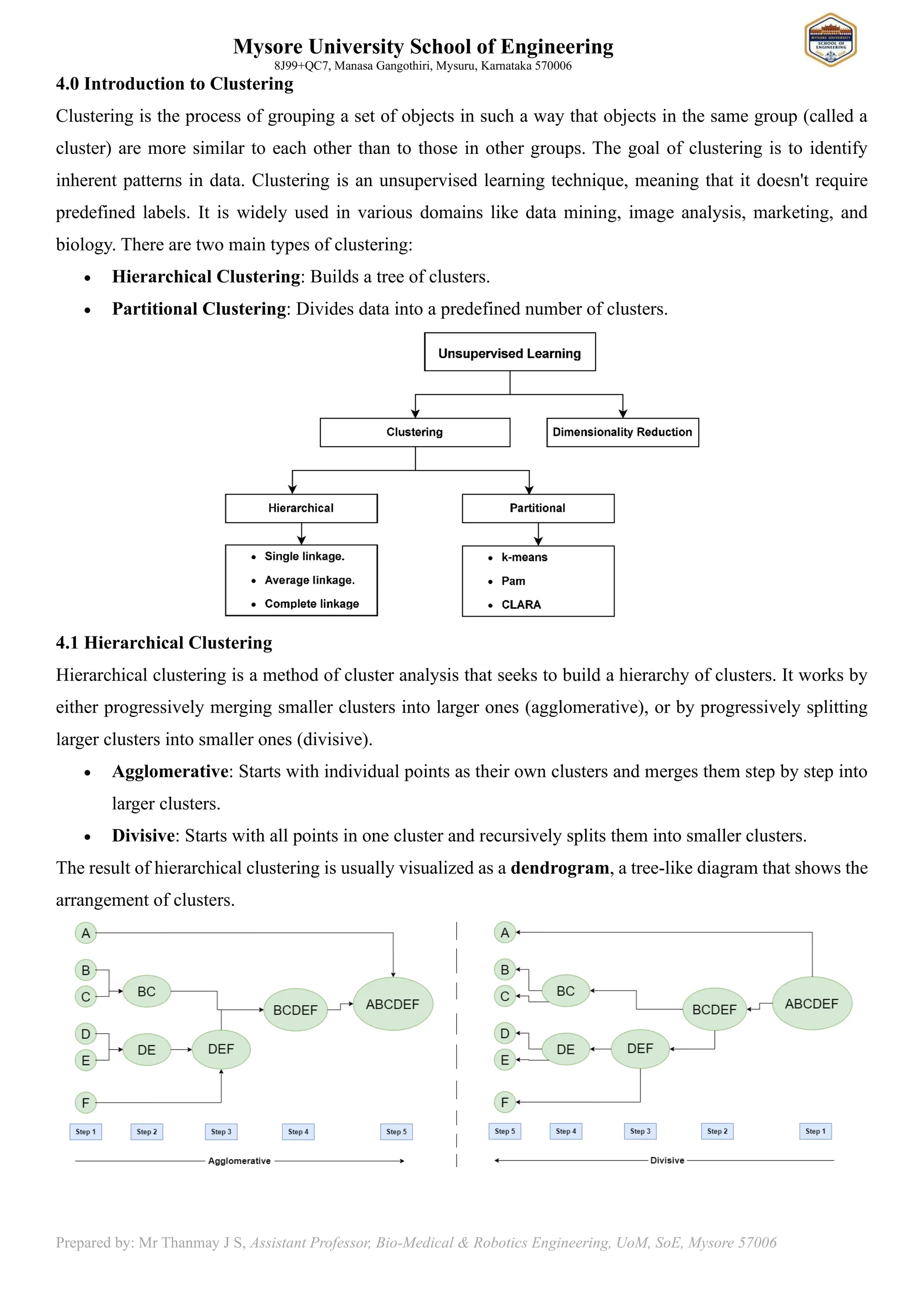
4.1 Hierarchical Clustering
Hierarchical clustering is a method of cluster analysis that seeks to build a hierarchy of clusters. It works by
either progressively merging smaller clusters into larger ones (agglomerative), or by progressively splitting
larger clusters into smaller ones (divisive).
• Agglomerative: Starts with individual points as their own clusters and merges them step by step into
larger clusters.
• Divisive: Starts with all points in one cluster and recursively splits them into smaller clusters.
The result of hierarchical clustering is usually visualized as a dendrogram, a tree-like diagram that shows the
arrangement of clusters.

4.2 Agglomerative Clustering Algorithms
Agglomerative clustering is a bottom-up approach. Initially, each data point is considered as its own cluster.
At each step, the closest (most similar) clusters are merged to form a larger cluster. The process continues until
all points are merged into one cluster or until a stopping criterion is met. The main steps in agglomerative
clustering are:
1. Initialize: Each data point is its own cluster.
2. Find closest clusters: Compute the distance between every pair of clusters.
3. Merge closest clusters: Merge the two clusters that are closest to each other.
4. Repeat: Repeat the process until only one cluster remains or a stopping criterion is reached.
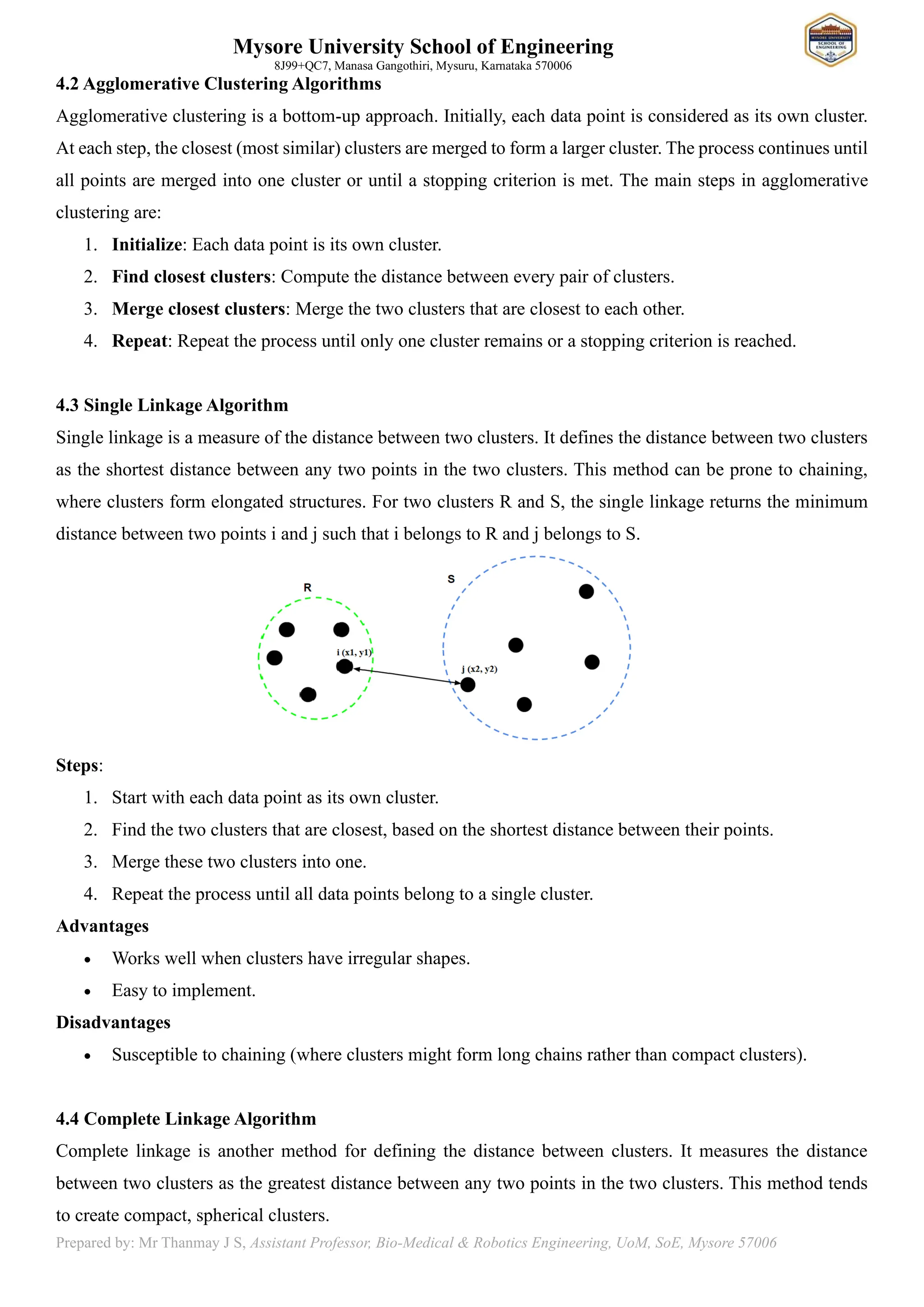
4.3 Single Linkage Algorithm
Single linkage is a measure of the distance between two clusters. It defines the distance between two clusters
as the shortest distance between any two points in the two clusters. This method can be prone to chaining,
where clusters form elongated structures. For two clusters R and S, the single linkage returns the minimum
distance between two points i and j such that i belongs to R and j belongs to S.
Steps:
1. Start with each data point as its own cluster.
2. Find the two clusters that are closest, based on the shortest distance between their points.
3. Merge these two clusters into one.
4. Repeat the process until all data points belong to a single cluster.
Advantages
• Works well when clusters have irregular shapes.
• Easy to implement.
Disadvantages
• Susceptible to chaining (where clusters might form long chains rather than compact clusters).
4.4 Complete Linkage Algorithm
Complete linkage is another method for defining the distance between clusters. It measures the distance
between two clusters as the greatest distance between any two points in the two clusters. This method tends
to create compact, spherical clusters.

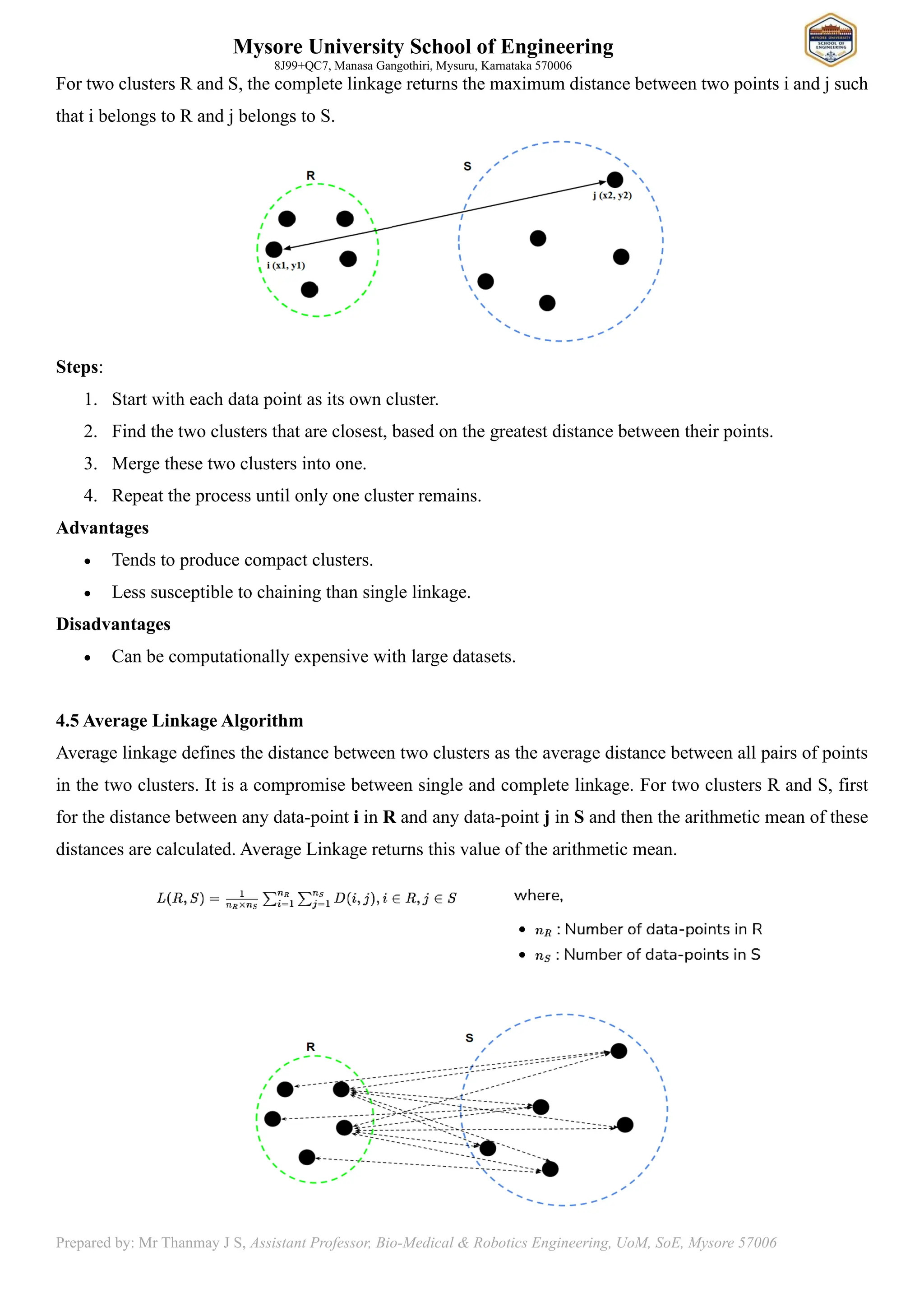
For two clusters R and S, the complete linkage returns the maximum distance between two points i and j such
that i belongs to R and j belongs to S.
Steps:
2. Find the two clusters that are closest, based on the greatest distance between their points.
3. Merge these two clusters into one.
4. Repeat the process until only one cluster remains.
Advantages
• Tends to produce compact clusters.
• Less susceptible to chaining than single linkage.
Disadvantages
• Can be computationally expensive with large datasets.
4.5 Average Linkage Algorithm
Average linkage defines the distance between two clusters as the average distance between all pairs of points
in the two clusters. It is a compromise between single and complete linkage. For two clusters R and S, first
for the distance between any data-point i in R and any data-point j in S and then the arithmetic mean of these
distances are calculated. Average Linkage returns this value of the arithmetic mean.

Steps:
2. Calculate the average distance between all points in the two clusters.
3. Merge the two clusters with the smallest average distance.
4. Repeat the process until one cluster remains.
Advantages
• Balances the advantages of both single and complete linkage.
• Works well for datasets with varying cluster shapes.
Disadvantages
• Can be more computationally intensive compared to single or complete linkage.
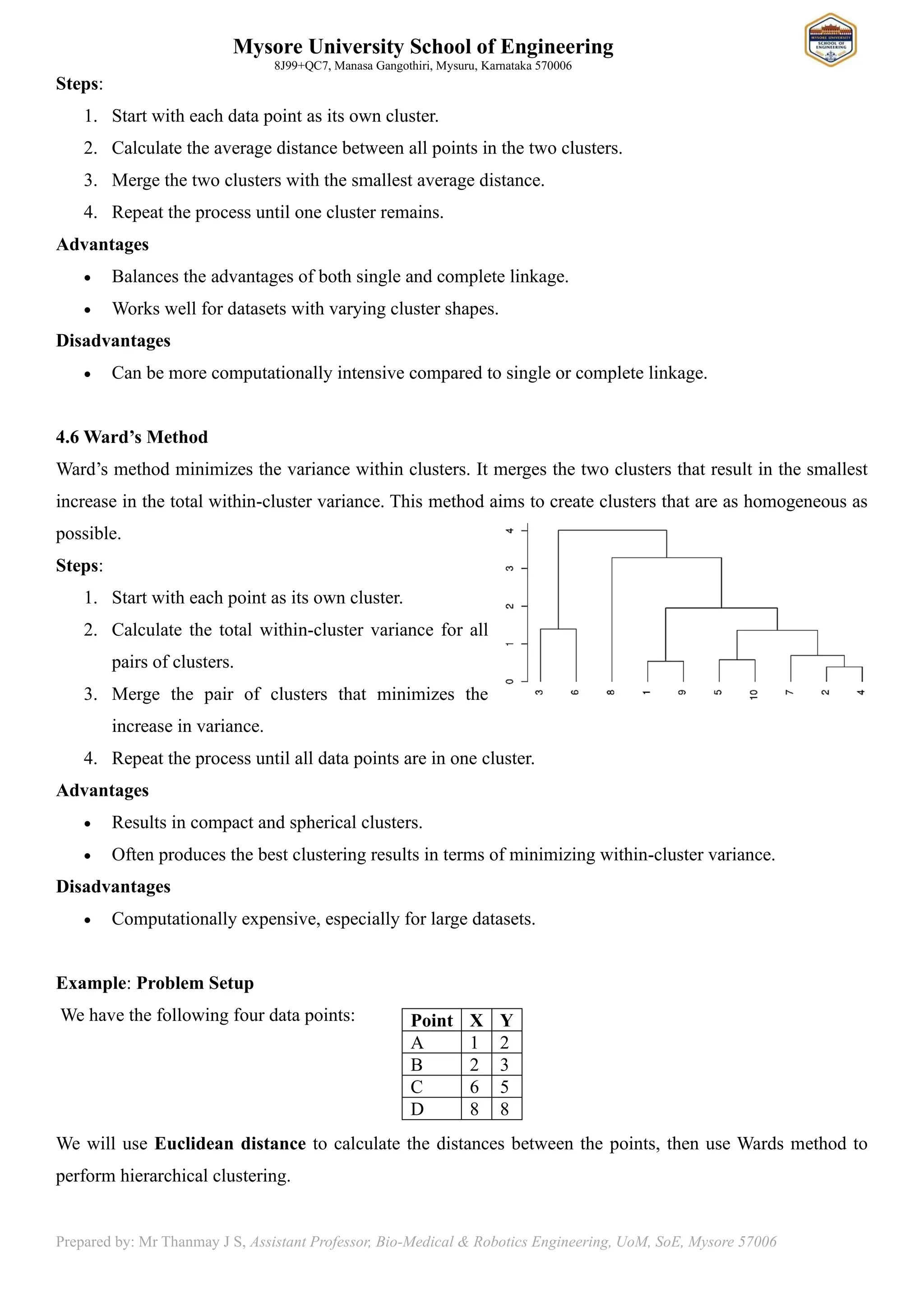
4.6 Ward’s Method
Ward’s method minimizes the variance within clusters. It merges the two clusters that result in the smallest
increase in the total within-cluster variance. This method aims to create clusters that are as homogeneous as
possible.
Steps:
1. Start with each point as its own cluster.
2. Calculate the total within-cluster variance for all
pairs of clusters.
3. Merge the pair of clusters that minimizes the
increase in variance.
4. Repeat the process until all data points are in one cluster.
Advantages
• Results in compact and spherical clusters.
• Often produces the best clustering results in terms of minimizing within-cluster variance.
Disadvantages
• Computationally expensive, especially for large datasets.
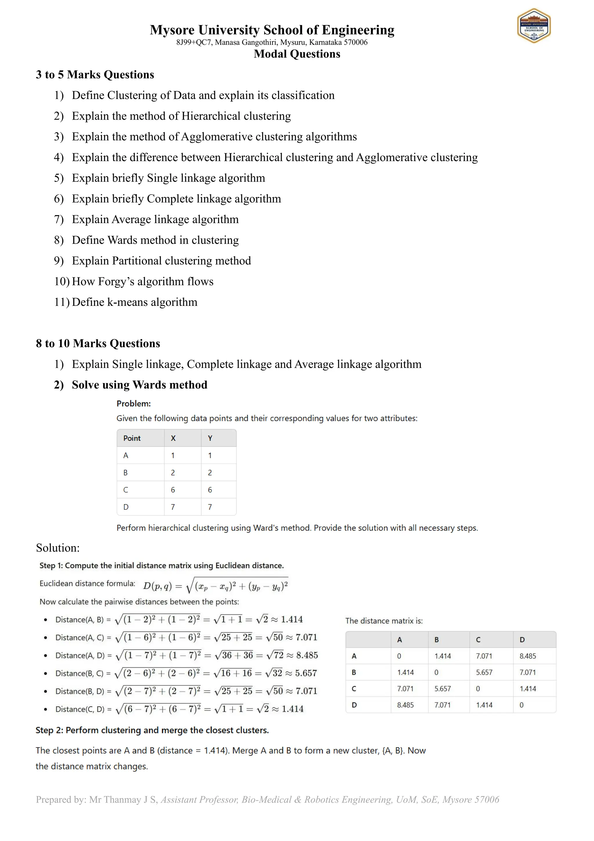
Example: Problem Setup
We have the following four data points:
We will use Euclidean distance to calculate the distances between the points, then use Wards method to
perform hierarchical clustering.
Point X Y
A 1 2
B 2 3
C 6 5
D 8 8

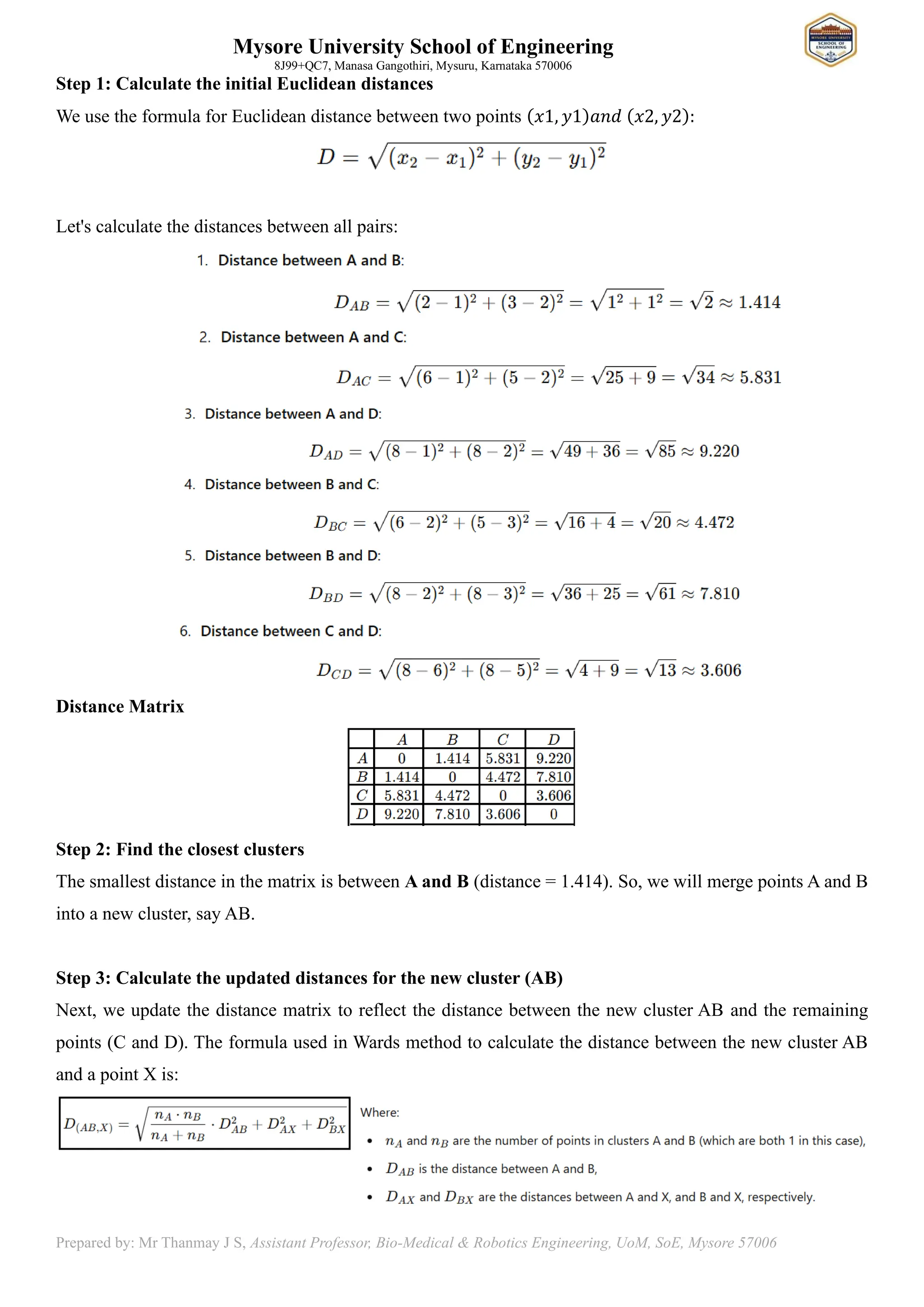
Step 1: Calculate the initial Euclidean distances
We use the formula for Euclidean distance between two points (𝑥1, 𝑦1)𝑎𝑛𝑑 (𝑥2, 𝑦2):
Let's calculate the distances between all pairs:
Distance Matrix
Step 2: Find the closest clusters
The smallest distance in the matrix is between A and B (distance = 1.414). So, we will merge points A and B
into a new cluster, say AB.
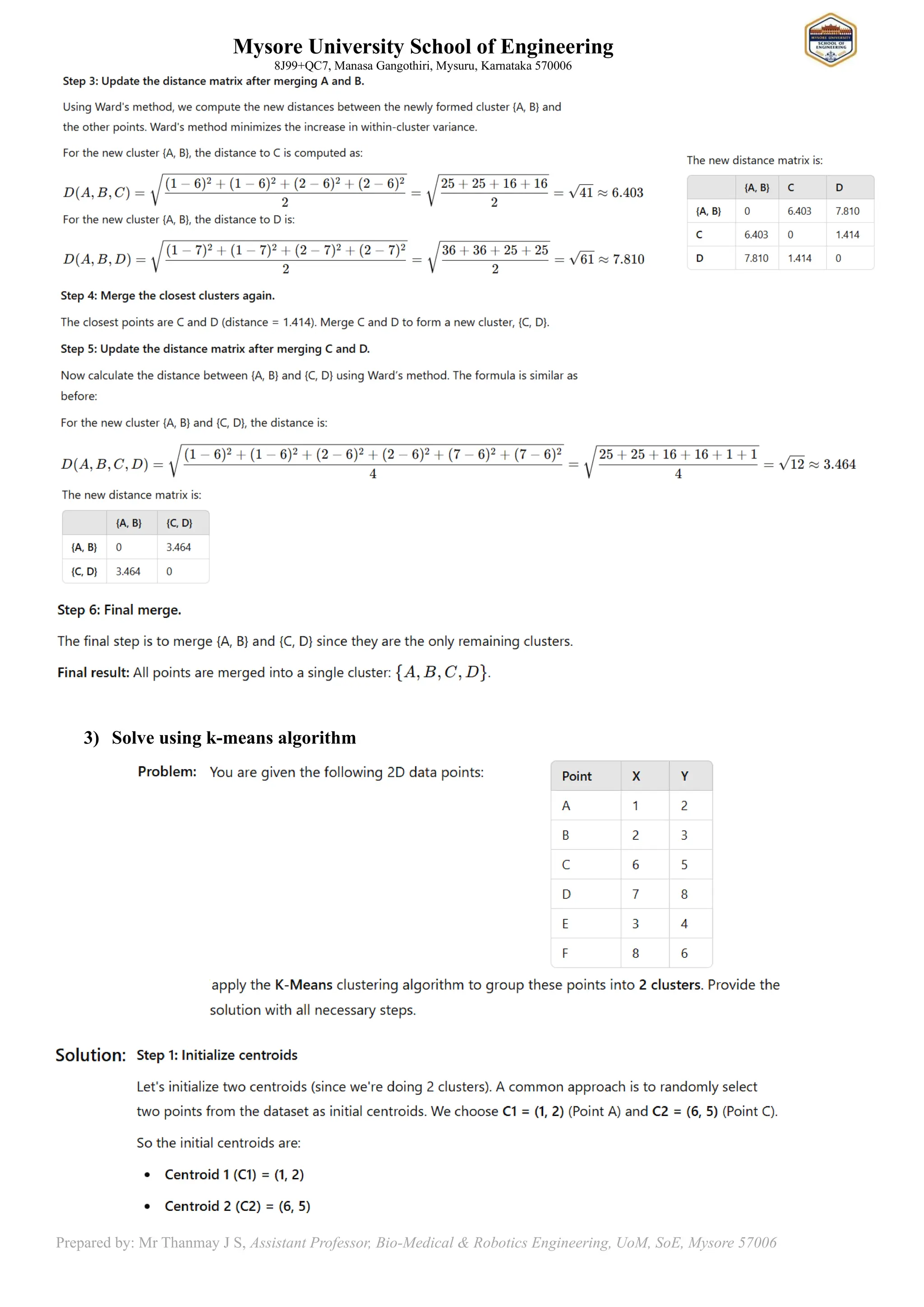
Step 3: Calculate the updated distances for the new cluster (AB)
Next, we update the distance matrix to reflect the distance between the new cluster AB and the remaining
points (C and D). The formula used in Wards method to calculate the distance between the new cluster AB
and a point X is:

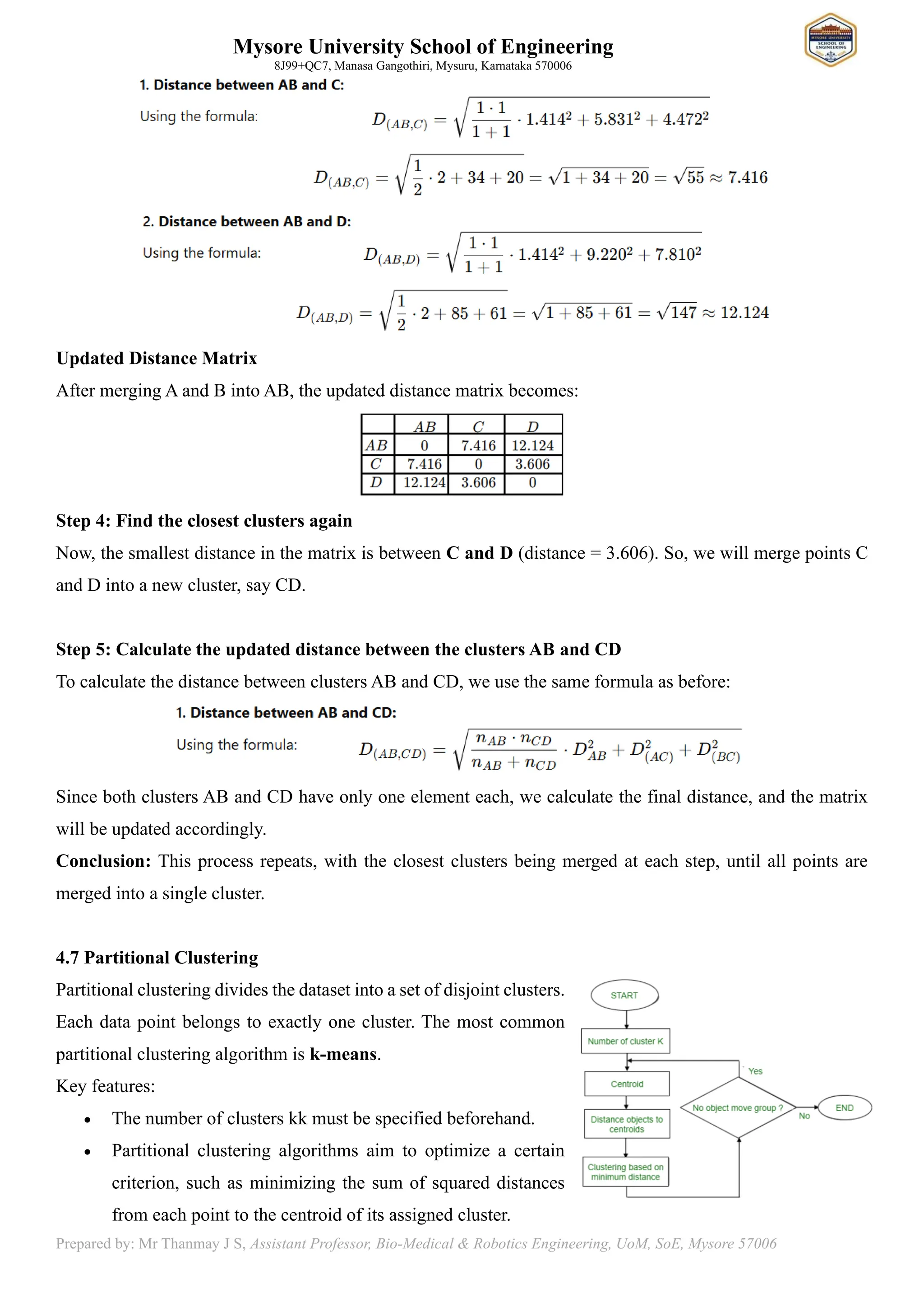
Updated Distance Matrix
After merging A and B into AB, the updated distance matrix becomes:
Step 4: Find the closest clusters again
Now, the smallest distance in the matrix is between C and D (distance = 3.606). So, we will merge points C
and D into a new cluster, say CD.
Step 5: Calculate the updated distance between the clusters AB and CD
To calculate the distance between clusters AB and CD, we use the same formula as before:
Since both clusters AB and CD have only one element each, we calculate the final distance, and the matrix
will be updated accordingly.
Conclusion: This process repeats, with the closest clusters being merged at each step, until all points are
merged into a single cluster.
4.7 Partitional Clustering
Partitional clustering divides the dataset into a set of disjoint clusters.
Each data point belongs to exactly one cluster. The most common
partitional clustering algorithm is k-means.
Key features:
• The number of clusters kk must be specified beforehand.
• Partitional clustering algorithms aim to optimize a certain
criterion, such as minimizing the sum of squared distances
from each point to the centroid of its assigned cluster.

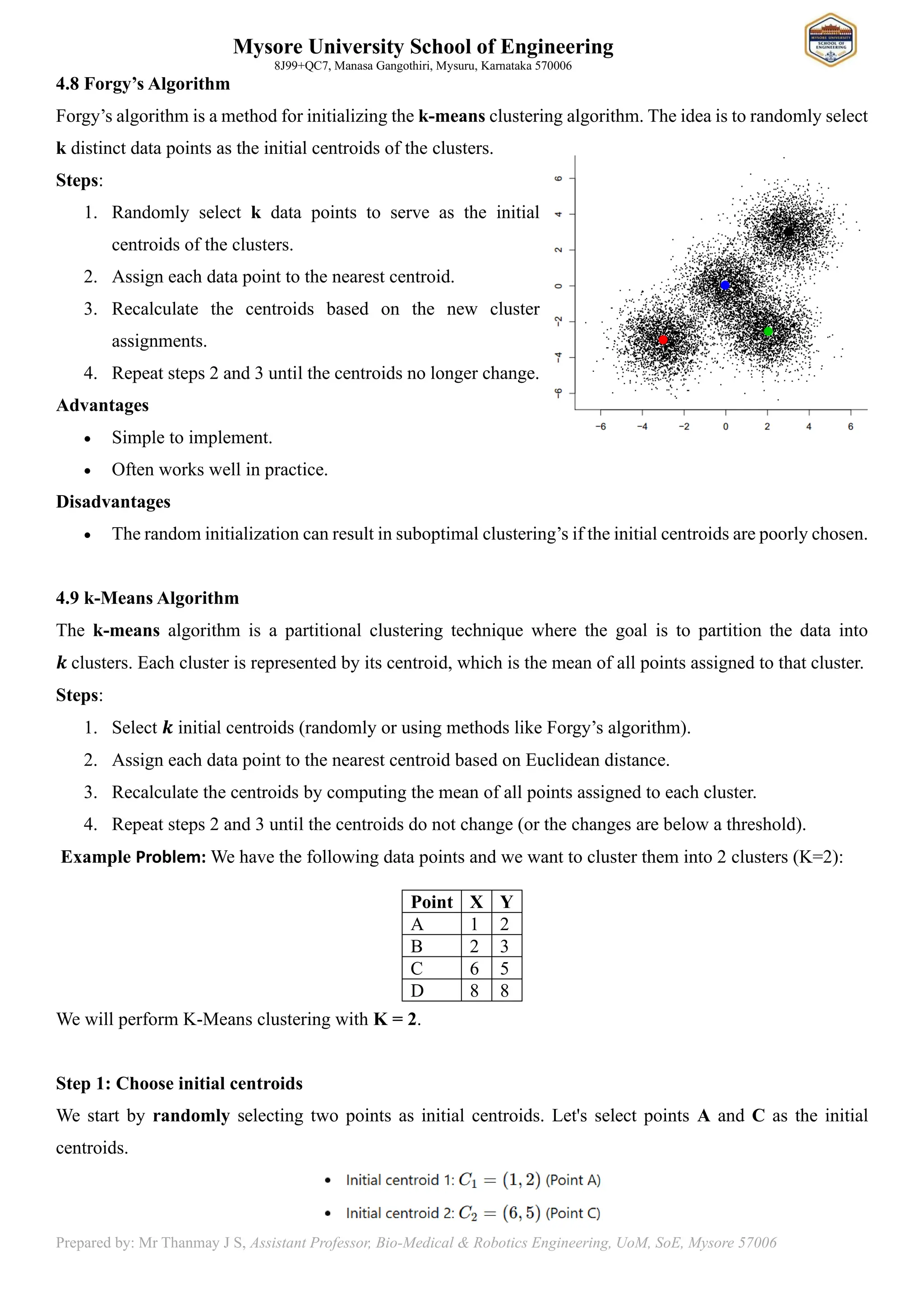
4.8 Forgy’s Algorithm
Forgy’s algorithm is a method for initializing the k-means clustering algorithm. The idea is to randomly select
k distinct data points as the initial centroids of the clusters.
Steps:
1. Randomly select k data points to serve as the initial
centroids of the clusters.
2. Assign each data point to the nearest centroid.
3. Recalculate the centroids based on the new cluster
assignments.
4. Repeat steps 2 and 3 until the centroids no longer change.
Advantages
• Simple to implement.
• Often works well in practice.
Disadvantages
• The random initialization can result in suboptimal clustering’s if the initial centroids are poorly chosen.
4.9 k-Means Algorithm
The k-means algorithm is a partitional clustering technique where the goal is to partition the data into
𝒌 clusters. Each cluster is represented by its centroid, which is the mean of all points assigned to that cluster.
Steps:
1. Select 𝒌 initial centroids (randomly or using methods like Forgy’s algorithm).
2. Assign each data point to the nearest centroid based on Euclidean distance.
3. Recalculate the centroids by computing the mean of all points assigned to each cluster.
4. Repeat steps 2 and 3 until the centroids do not change (or the changes are below a threshold).
Example Problem: We have the following data points and we want to cluster them into 2 clusters (K=2):
We will perform K-Means clustering with K = 2.
Step 1: Choose initial centroids
We start by randomly selecting two points as initial centroids. Let's select points A and C as the initial
centroids.
Point X Y
A 1 2
B 2 3
C 6 5
D 8 8

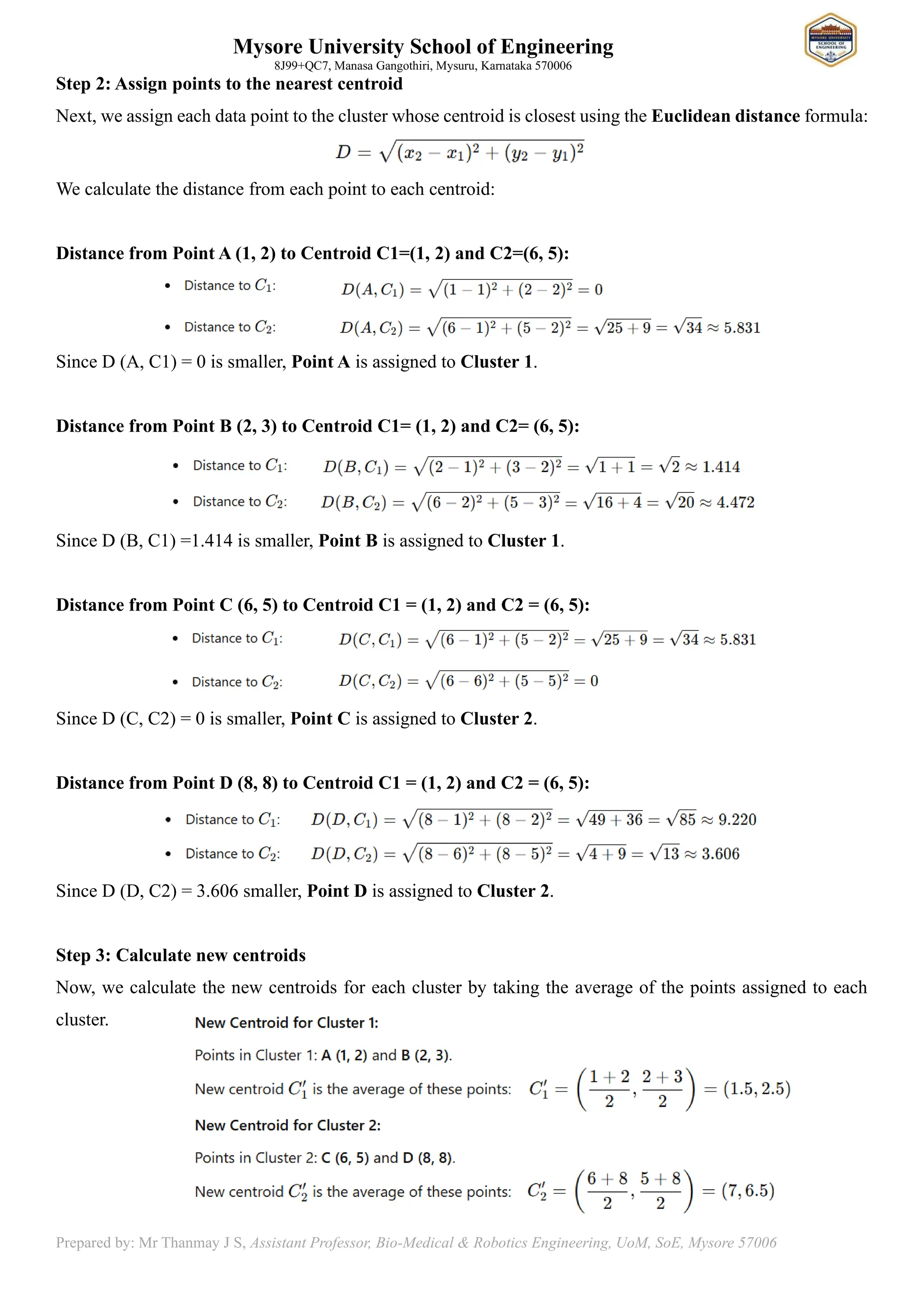
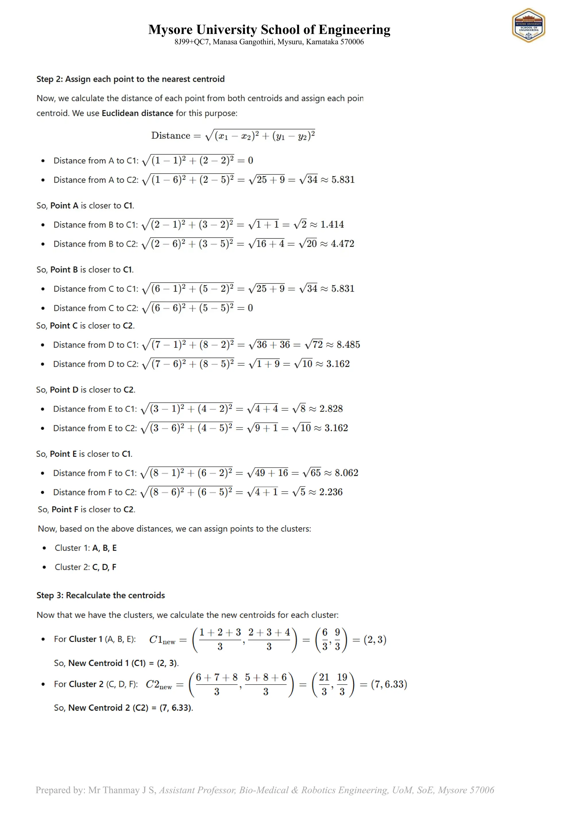
Step 2: Assign points to the nearest centroid
Next, we assign each data point to the cluster whose centroid is closest using the Euclidean distance formula:
We calculate the distance from each point to each centroid:
Distance from Point A (1, 2) to Centroid C1=(1, 2) and C2=(6, 5):
Since D (A, C1) = 0 is smaller, Point A is assigned to Cluster 1.
Distance from Point B (2, 3) to Centroid C1= (1, 2) and C2= (6, 5):
Since D (B, C1) =1.414 is smaller, Point B is assigned to Cluster 1.
Distance from Point C (6, 5) to Centroid C1 = (1, 2) and C2 = (6, 5):
Since D (C, C2) = 0 is smaller, Point C is assigned to Cluster 2.
Distance from Point D (8, 8) to Centroid C1 = (1, 2) and C2 = (6, 5):
Since D (D, C2) = 3.606 smaller, Point D is assigned to Cluster 2.
Step 3: Calculate new centroids
Now, we calculate the new centroids for each cluster by taking the average of the points assigned to each
cluster.

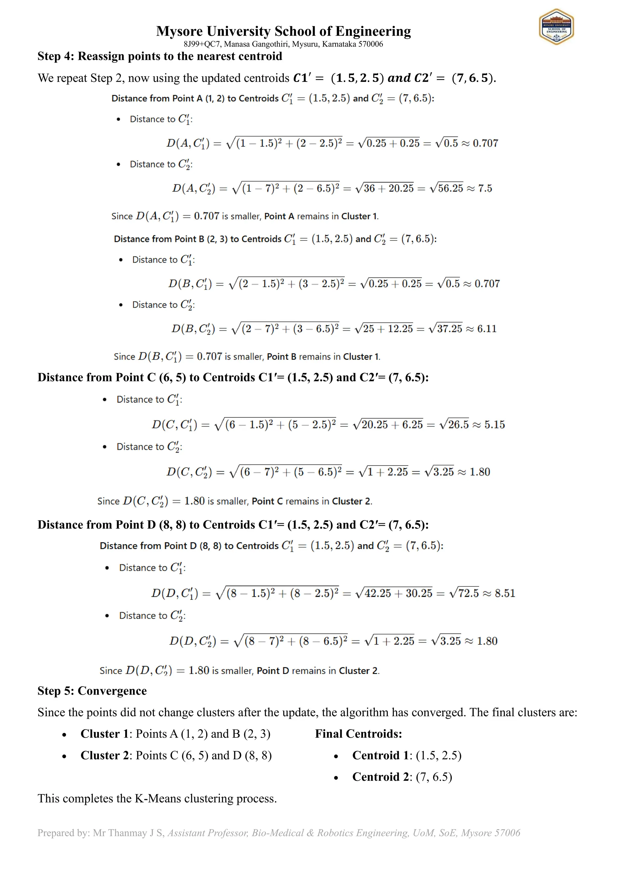
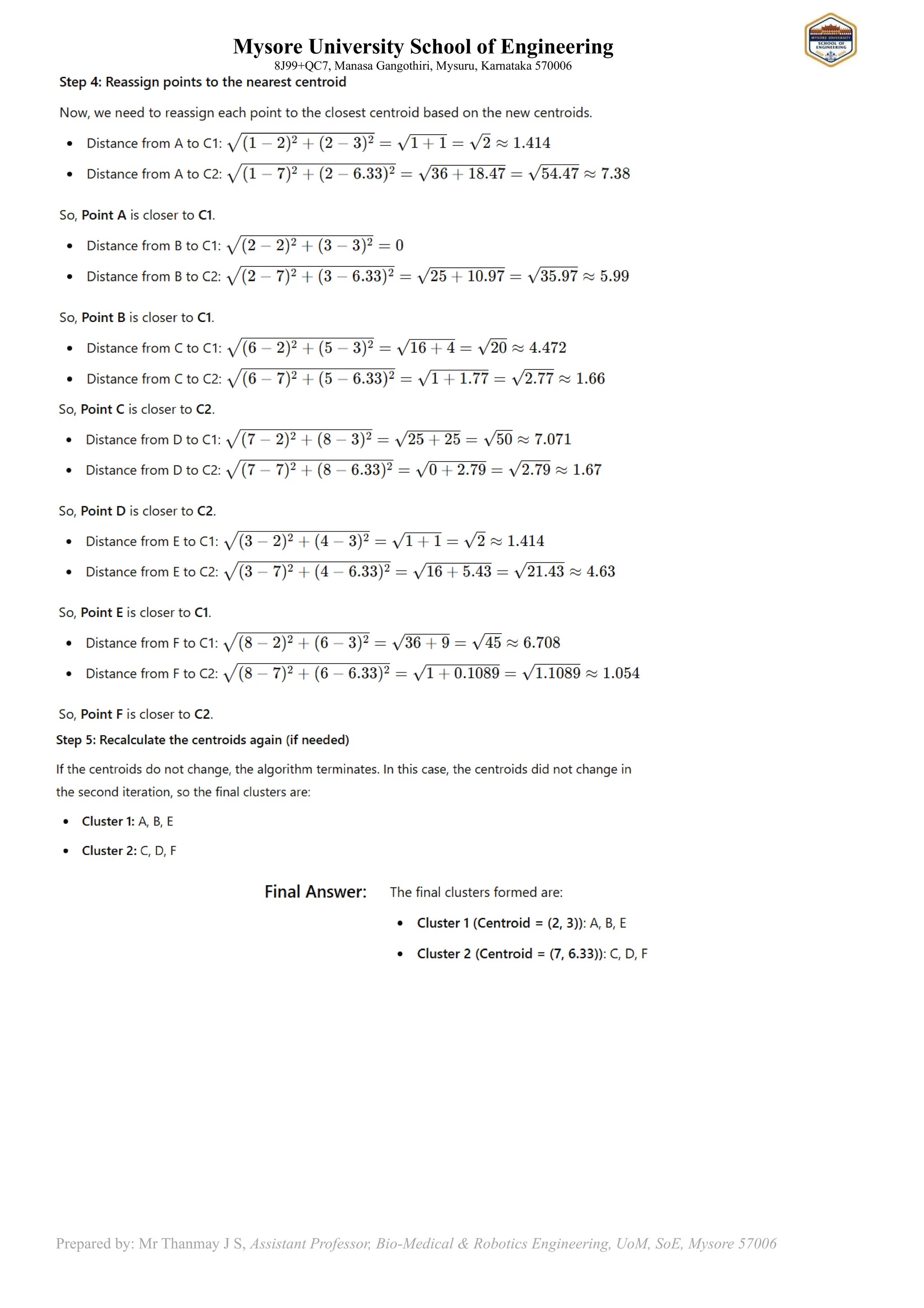
Step 4: Reassign points to the nearest centroid
We repeat Step 2, now using the updated centroids 𝑪𝟏′ = (𝟏. 𝟓, 𝟐. 𝟓) 𝒂𝒏𝒅 𝑪𝟐′ = (𝟕, 𝟔. 𝟓).
Distance from Point C (6, 5) to Centroids C1′= (1.5, 2.5) and C2′= (7, 6.5):
Distance from Point D (8, 8) to Centroids C1′= (1.5, 2.5) and C2′= (7, 6.5):
Step 5: Convergence
Since the points did not change clusters after the update, the algorithm has converged. The final clusters are:
• Cluster 1: Points A (1, 2) and B (2, 3)
• Cluster 2: Points C (6, 5) and D (8, 8)
Final Centroids:
• Centroid 1: (1.5, 2.5)
• Centroid 2: (7, 6.5)
This completes the K-Means clustering process.

Advantages
• Simple and efficient.
• Works well with large datasets.
Disadvantages
• Requires the number of clusters k to be specified beforehand.
• Sensitive to the initial selection of centroids.
• Struggles with clusters of different sizes, densities, and shapes.

Modal Questions
3 to 5 Marks Questions
1) Define Clustering of Data and explain its classification
2) Explain the method of Hierarchical clustering
3) Explain the method of Agglomerative clustering algorithms
4) Explain the difference between Hierarchical clustering and Agglomerative clustering
5) Explain briefly Single linkage algorithm
6) Explain briefly Complete linkage algorithm
7) Explain Average linkage algorithm
8) Define Wards method in clustering
9) Explain Partitional clustering method
10) How Forgy’s algorithm flows
11) Define k-means algorithm
8 to 10 Marks Questions
1) Explain Single linkage, Complete linkage and Average linkage algorithm
2) Solve using Wards method
Solution:

3) Solve using k-means algorithm

Pattern Recognition 21BR551 MODULE 04 NOTES.pdf

More Related Content

Similar to Pattern Recognition 21BR551 MODULE 04 NOTES.pdf

More from THANMAY JS

Recently uploaded

Pattern Recognition 21BR551 MODULE 04 NOTES.pdf