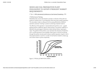
1. A partition curve shows the percentage of material from a feed that reports to either the sink or float product of a dense medium separation vessel, plotted against the nominal specific gravity of the material.
2. The partition curve can be determined by sampling the sink and float products, performing heavy liquid tests to determine the material distribution across density fractions, and calculating the partition coefficient for each fraction.
3. Partition curves are specific to a particular vessel and feed conditions, and can be used to predict separation performance and product distributions if those conditions change.
![6/20/22, 10:20 AM Partition Curve - an overview | ScienceDirect Topics
https://www.sciencedirect.com/topics/engineering/partition-curve#:~:text=The partition curve for an,of the dense medium unit. 9/38
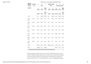
(11.5)
(11.6)
(11.7)
(11.8)
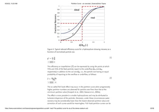
normalized density, ρ/ρ , where ρ is the separating density (RD ). The
normalized curve is generally independent of cut-point and medium density, but is
dependent on particle size. Inserting this normalized density into Eq. (11.4), and
noting that P=50 for ρ=ρ (ρ/ρ =1), gives:
One of the advantages of Eq. (11.5) is that it can be linearized so that simple linear
regression can be used to estimate m and ρ from experimental data:
(This approach is less important today with any number of curve-fitting routines
available (and Excel Solver), the same point also made in Chapter 9 when curve-
fitting cyclone partition curves.)
Gottfried (1978) proposed a related function, the Weibull function, with additional
parameters to account for the fact that the curves do not always reach the 0 and
100% asymptotes due to short-circuit flow:
The six parameters of the function (c, f , ρ , x , a, and b) are not independent, so
by the argument of Eq. (11.5), x can be expressed as:
In this version of the function, representing percentage of feed to sinks, f is the
proportion of high-density material misplaced to floats, and 1−(c+f ) is the
proportion of low-density material misplaced to sinks, so that c+f ≤1. The curve
therefore varies from a minimum of 100[1−(c+f )] to a maximum of 100(1−f ).
The parameters of Eq. (11.8) have to be determined by nonlinear estimation. First
approximations of c, f , and ρ can be obtained from the curve itself.
King and Juckes (1988) used Whiten’s classification function (Lynch, 1977) with two
additional parameters to describe the short-circuit flows or by-pass:
50 50 50
50 50
50
0 50 0
0
0
0
0
0 0
0 50](https://image.slidesharecdn.com/partitioncurve-anoverviewsciencedirecttopics1-220816114447-14a2941e/85/Partition-Curve-an-overview-_-ScienceDirect-Topics-1-pdf-9-320.jpg)
![6/20/22, 10:20 AM Partition Curve - an overview | ScienceDirect Topics
https://www.sciencedirect.com/topics/engineering/partition-curve#:~:text=The partition curve for an,of the dense medium unit. 21/38
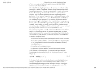
(3)
modelled by summation of a corrected partition curve (such as represented by
Eqn(3)) and the product of an inverted partition curve and a bypass fraction
(Cilliers, 2000).
Read full chapter
URL: https://www.sciencedirect.com/science/article/pii/B978012384746100001X
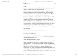
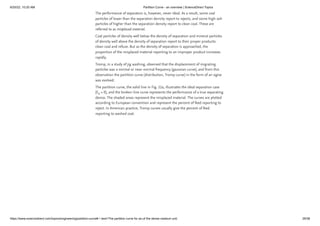
Gravity Separation
In Mineral Processing Design and Operations (Second Edition), 2016
16.8.4 Sink-Float Alternatives
Because of the importance of washability and sink-float analysis to the coal industry
and the health hazards associated with the presence of organic liquids,
considerable effort is being aimed at alternatives to the organic liquid method. To
determine the partition curve of a gravity separation unit, density tracers may be
used. These are plastic particles manufactured to precise density such as 0.005 SG
units [25]. These tracers are available in cubic shape from 1 to 64 mm or as crushed
particles to simulate real ore with sizes from 0.125 to 32 mm or more. Density
ranges are from 1.24 to 4.5 S.G. and can be colour coded or made magnetic or
fluorescent for ease of recovery. A range of tracers of different density and size are
added to the unit feed and retrieved from the floats and sinks fractions. The ratio of
numbers in the floats and feed will give the partition coefficient.
For an alternative to the sink-float analysis, the Julius Kruttschnitt Mineral Research
Centre (JKMRC) have developed an automatic gas pycnometer in which the dry
density of individual particles is determined by separate mass and volume
measurements [26]. The instrument is capable of analyzing 30 particles a minute. A
sink-float data analysis requiring about 3000 particles can be obtained in 100 min.
Read full chapter
URL: https://www.sciencedirect.com/science/article/pii/B9780444635891000162](https://image.slidesharecdn.com/partitioncurve-anoverviewsciencedirecttopics1-220816114447-14a2941e/85/Partition-Curve-an-overview-_-ScienceDirect-Topics-1-pdf-21-320.jpg)
![6/20/22, 10:20 AM Partition Curve - an overview | ScienceDirect Topics
https://www.sciencedirect.com/topics/engineering/partition-curve#:~:text=The partition curve for an,of the dense medium unit. 24/38
[17.2]
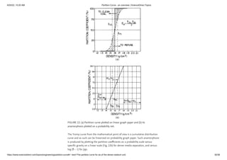
In some countries, partition curves are plotted as RD vs the probability of reporting
to refuse. This convention provides a mirror image of the partition curve based on
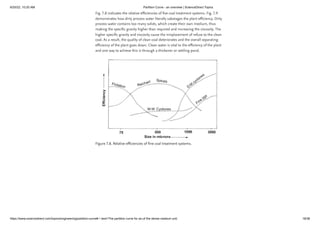
clean coal partitioning.) The steepness of the partition curve, which reflects the
sharpness of the separation, is typically reported using an Ecart Probable (Ep) value
defined as:
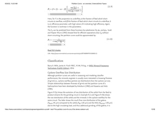
Figure 17.4. Partition curves for (a) perfect and (b) imperfect separations.
in which RD and RD are the relative densities that correspond to probabilities
of 25% and 75%. A lower Ep is desirable, since it means that fewer particles are
misplaced during the separation.
25 75](https://image.slidesharecdn.com/partitioncurve-anoverviewsciencedirecttopics1-220816114447-14a2941e/85/Partition-Curve-an-overview-_-ScienceDirect-Topics-1-pdf-24-320.jpg)
![6/20/22, 10:20 AM Partition Curve - an overview | ScienceDirect Topics
https://www.sciencedirect.com/topics/engineering/partition-curve#:~:text=The partition curve for an,of the dense medium unit. 25/38
[17.3]
[17.4]
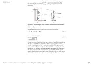
Several detailed methods have been reported in the literature for establishing
partition curves (Luckie et al., 1969). However, the fastest and simplest method
involves the collection of representative samples of the feed, clean and refuse
streams around the cleaning unit. Once collected, the samples are dried and
representative splits subjected to ash analysis. From the ash values, the ratio (Z) of
reject tonnage to clean tonnage can be calculated using:
in which f, c, and r are the feed, clean, and refuse ash contents, respectively. For
example, the Z ratio for a dense medium separator coal treating a 25% feed ash
and generating a 10% clean ash and 70% reject ash would be:
This calculation indicates that 0.333 tons of reject would be generated for each ton
of clean coal. Representative splits of clean coal and refuse are then subjected to
float–sink (washability) testing. The float–sink tests provide the mass percent of dry
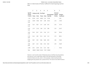
solids present in each density fraction. The first three columns of data in Table 17.3
(Columns 1–3) provide an example of the types of data obtained from such an
exercise. From these data, the partition factor (P) for each density class can be
quickly calculated using:
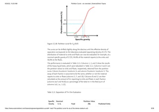
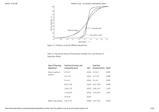
Table 17.3. Example of calculations for partition curve construction
Average RD Clean mass (%) Refuse mass (%) Partition factor
1.40 78.3 0.6 1.00
1.55 19.3 1.7 0.97
1.65 2.0 4.4 0.58
1.75 0.3 15.3 0.06
1 2 3 4](https://image.slidesharecdn.com/partitioncurve-anoverviewsciencedirecttopics1-220816114447-14a2941e/85/Partition-Curve-an-overview-_-ScienceDirect-Topics-1-pdf-25-320.jpg)
![6/20/22, 10:20 AM Partition Curve - an overview | ScienceDirect Topics
https://www.sciencedirect.com/topics/engineering/partition-curve#:~:text=The partition curve for an,of the dense medium unit. 26/38
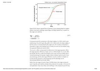
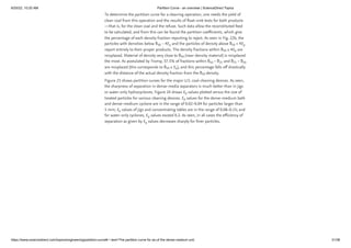
[17.5]
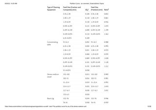
1.90 0.1 78.0 0.00
Totals 100.0 100.0 –
Column 4 = 1/(1 + Z (Column 3/Column 2)
Z = (Feed Ash – Clean Ash)/(Refuse Ash – Feed Ash).
in which R and C are the respective weight percentages of reject and clean coal in
each density class. In this case, the partition factor (P) represents the probability
that material of a given density in the feed will report to clean coal. These values,
which are listed in Column 4 for the example shown, were calculated as follows:
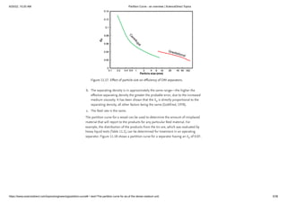
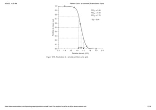
As shown in Fig. 17.5, the partition curve for the separator can be constructed by
plotting the partition factors (Column 4) as a function of the average RD of each
class (Column 1). For the example shown, the cutpoint (RD ) is 1.66 RD, which
corresponds to particles having an equal chance of reporting to either the clean or
reject streams. The Ep value is 0.04 (i.e., (1.70 – 1.62)/2 = 0.04), which can be
compared with tabular values, such as those shown in Fig. 17.6, to determine
whether the level of performance is acceptable for the equipment and size fraction
being evaluated.
1 2 3 4
50](https://image.slidesharecdn.com/partitioncurve-anoverviewsciencedirecttopics1-220816114447-14a2941e/85/Partition-Curve-an-overview-_-ScienceDirect-Topics-1-pdf-26-320.jpg)
![6/20/22, 10:20 AM Partition Curve - an overview | ScienceDirect Topics
https://www.sciencedirect.com/topics/engineering/partition-curve#:~:text=The partition curve for an,of the dense medium unit. 32/38
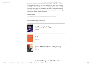
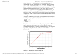
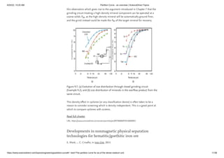
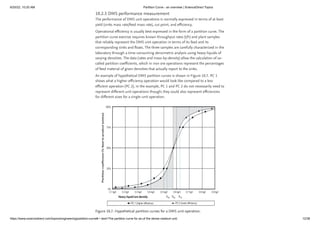
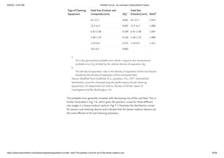
FIGURE 23. Performance of gravity separators. ▴, hydrocyclones, in. ×200 mesh;
▿, air tables, 2 in.×200 mesh; •, jigs: Baum, 6 in.× in.; Batac in.×28 mesh; □,
concentrating tables, in.×200 mesh; ○, dense-medium separators: cyclone,
in.×28 mesh; vessel, 6 in.× in. [From Killmeyer, R. P. “Performance characteristics
of coal-washing equipment: Baum and Batac jigs,” U.S. Department of Energy, RI-
PMTC-9(80).]](https://image.slidesharecdn.com/partitioncurve-anoverviewsciencedirecttopics1-220816114447-14a2941e/85/Partition-Curve-an-overview-_-ScienceDirect-Topics-1-pdf-32-320.jpg)
![6/20/22, 10:20 AM Partition Curve - an overview | ScienceDirect Topics
https://www.sciencedirect.com/topics/engineering/partition-curve#:~:text=The partition curve for an,of the dense medium unit. 33/38
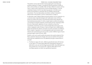
(6)
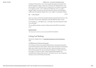
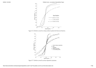
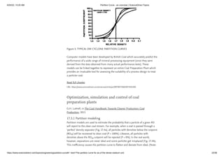
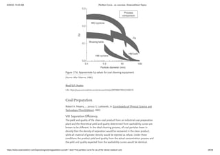
FIGURE 24. Probable error E vs mean size of the treated coal for dense-media
baths (DMB), dense-media cyclones (DMC), jigs, concentrating tables, and water-
only cyclones (WOC). [After Mikhail, M. W., Picard, J. L., and Humeniuk, O. E.
(1982). “Performance evaluation of gravity separators in Canadian washeries.”
Paper presented at 2nd Technical Conference on Western Canadian Coals, Edmonton,
June 3–5.].
Another index developed to characterize the sharpness of separation is the
imperfection I.
for dense-medium separation, and
p](https://image.slidesharecdn.com/partitioncurve-anoverviewsciencedirecttopics1-220816114447-14a2941e/85/Partition-Curve-an-overview-_-ScienceDirect-Topics-1-pdf-33-320.jpg)