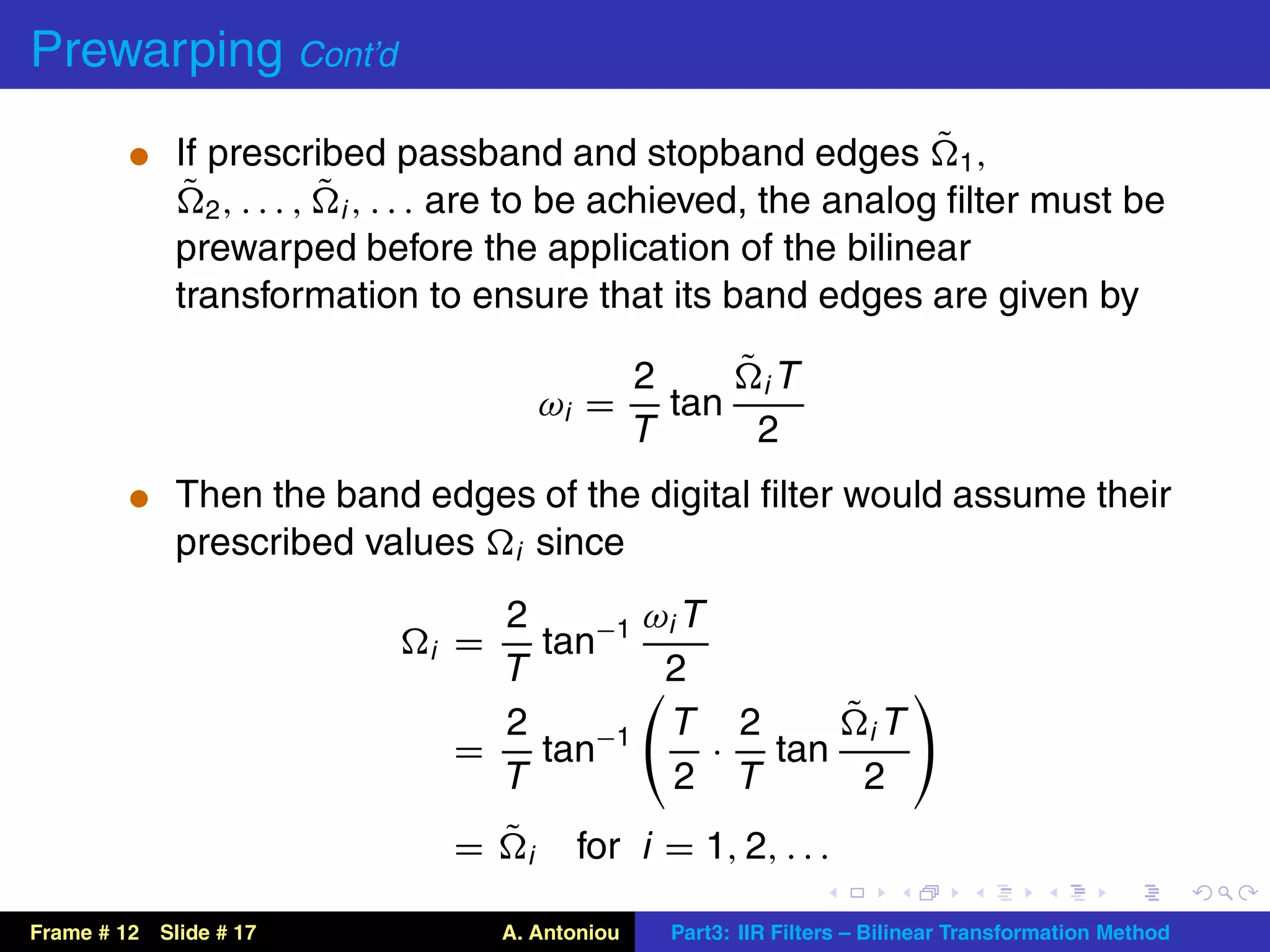
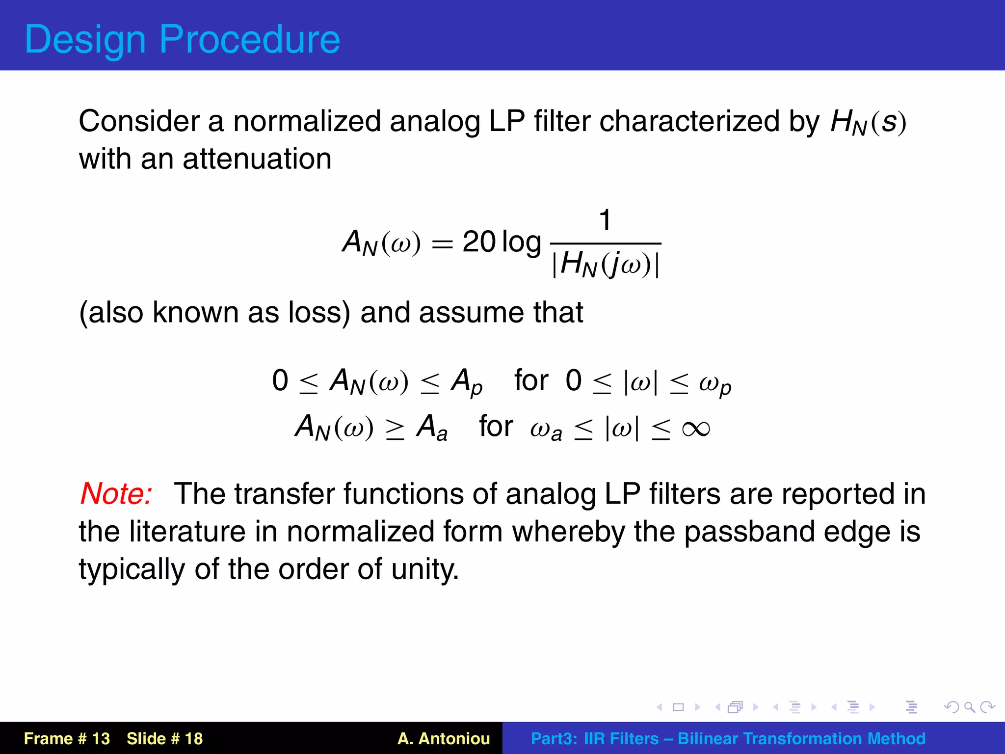
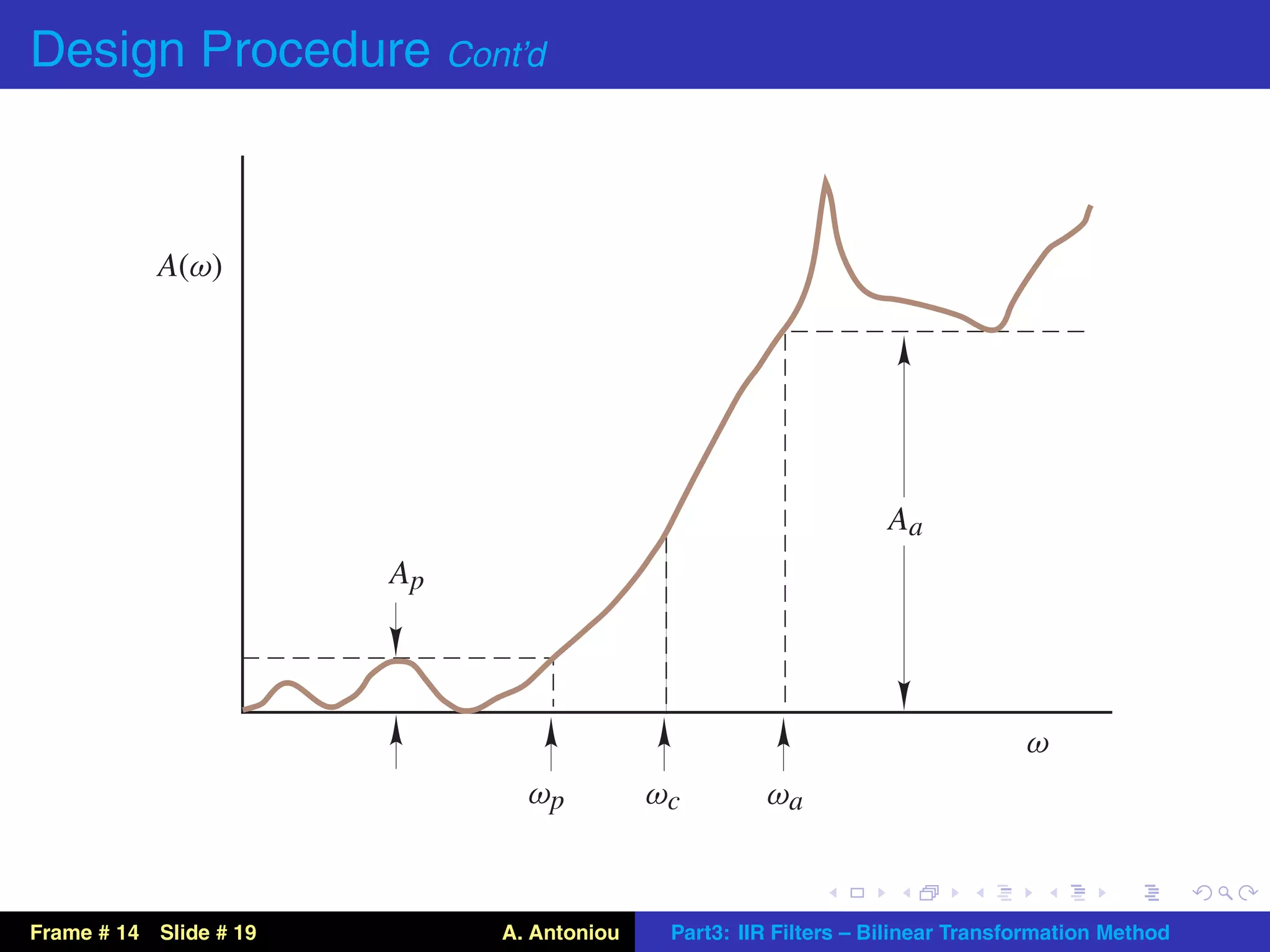
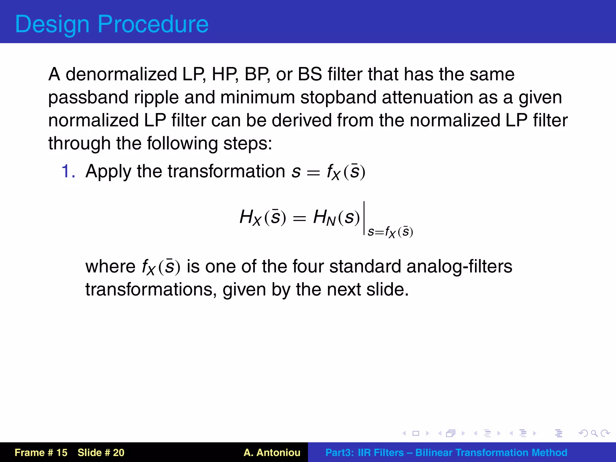
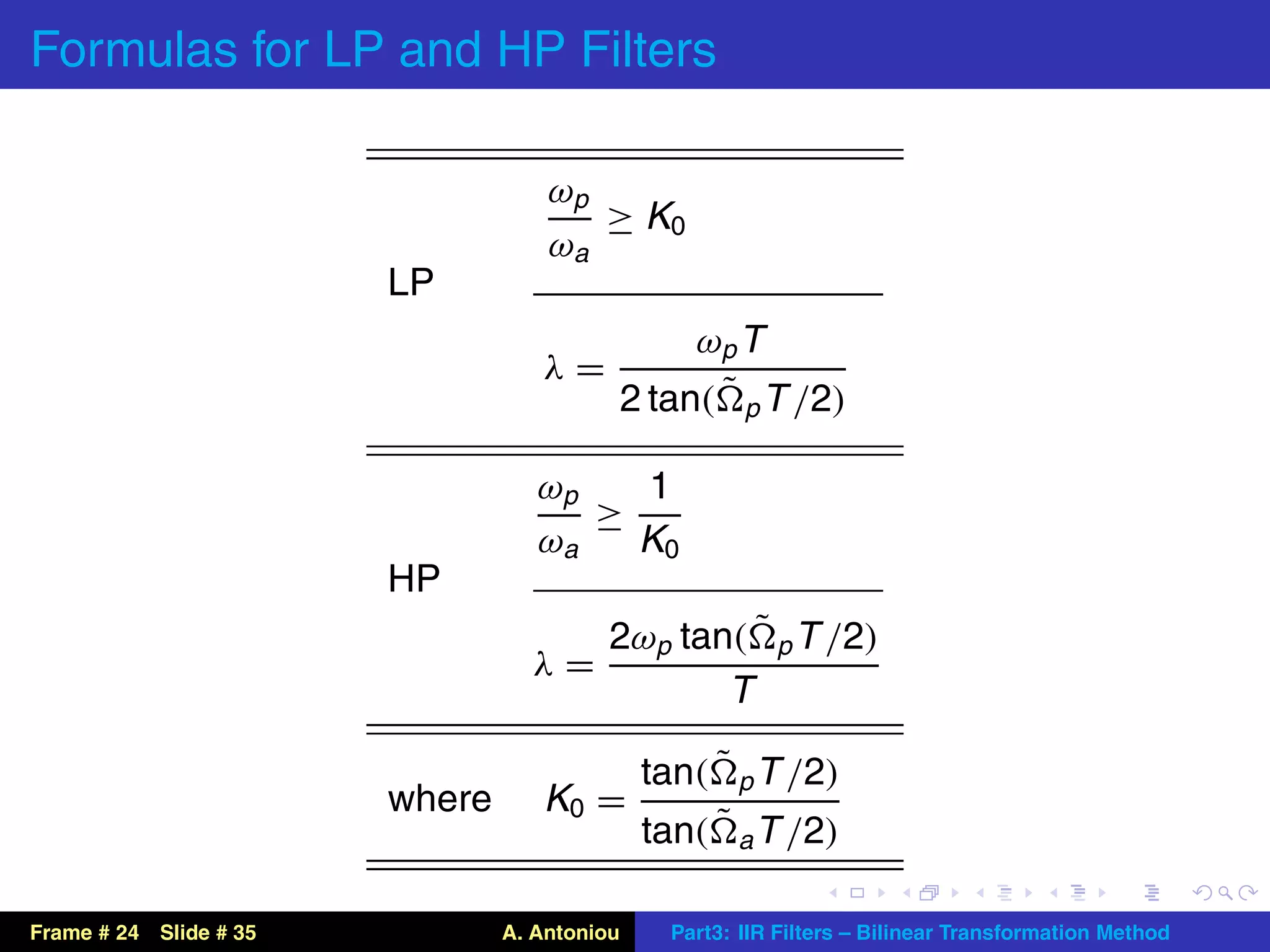
Download as PDF, PPTX
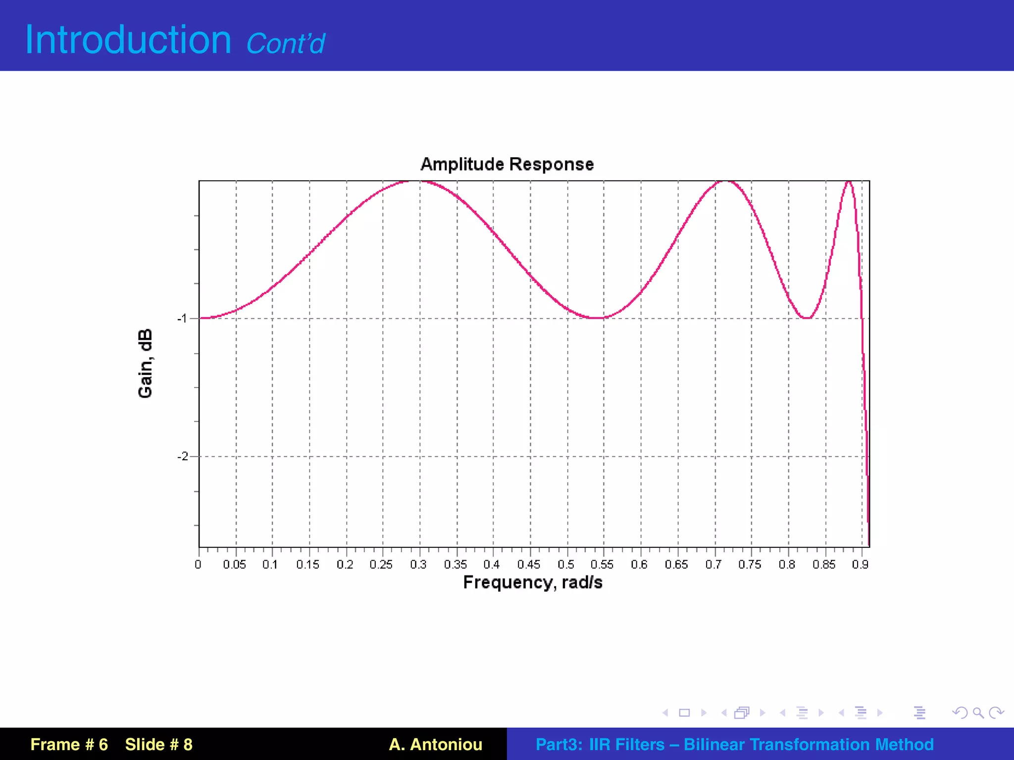
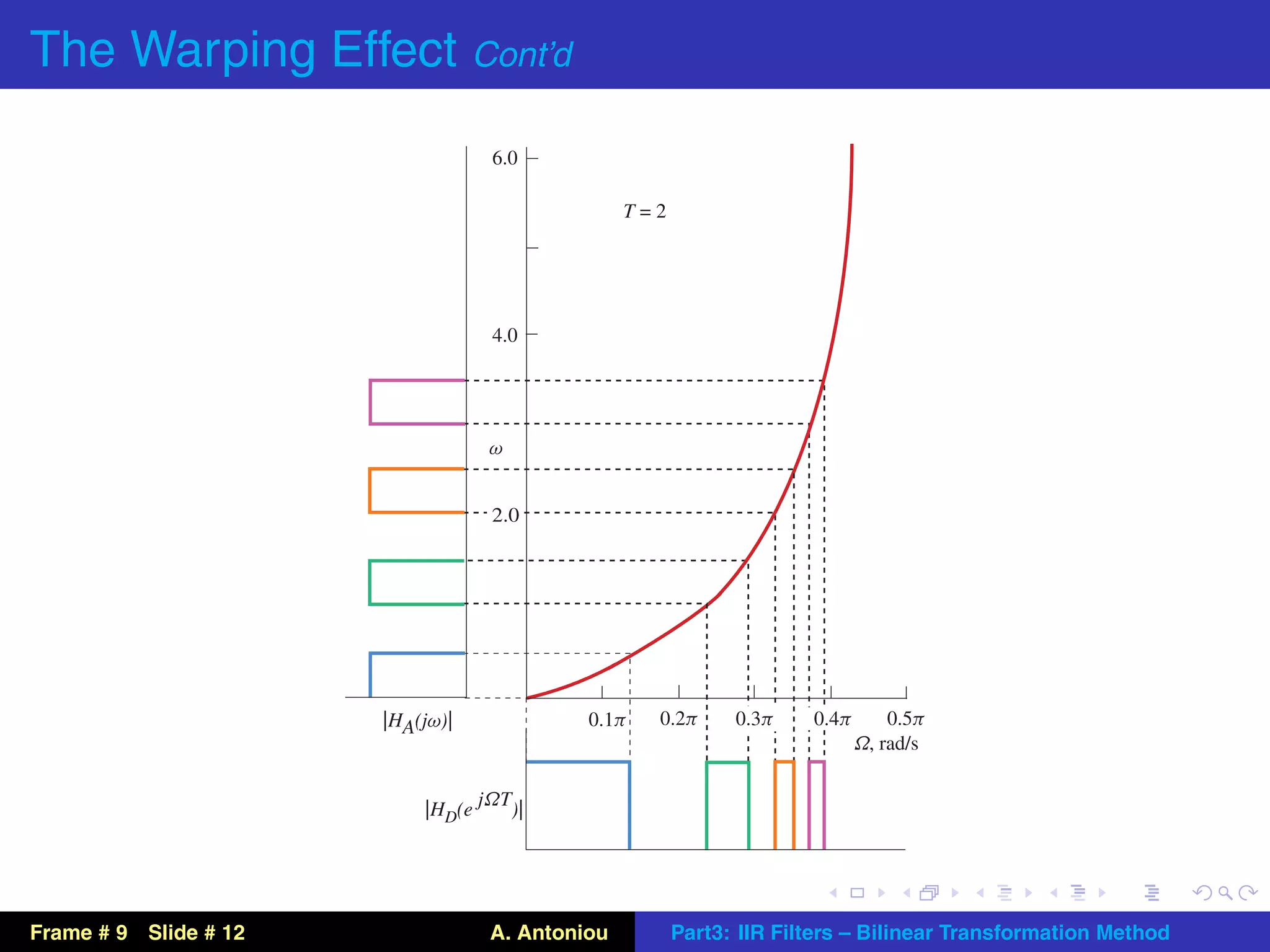
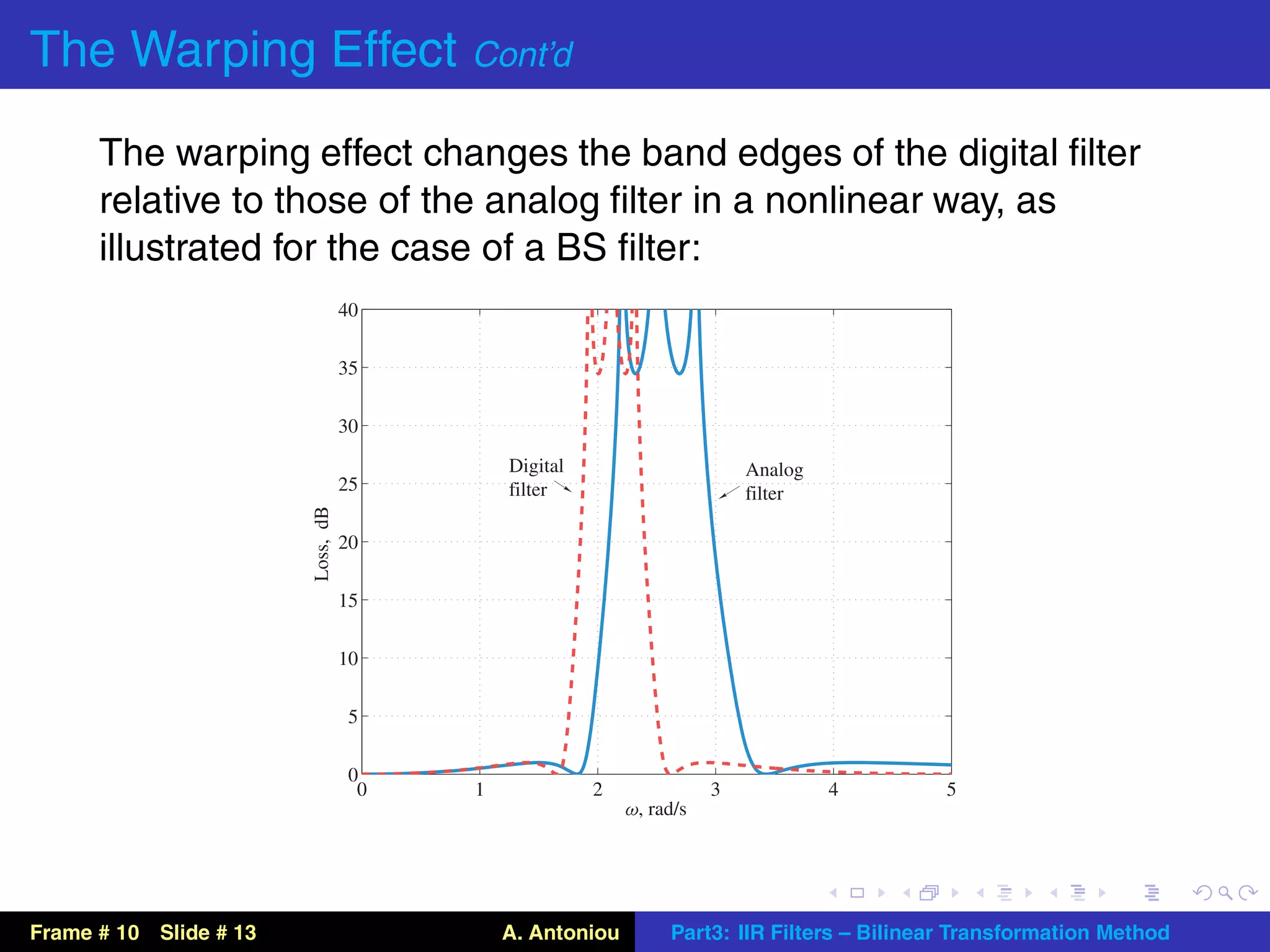
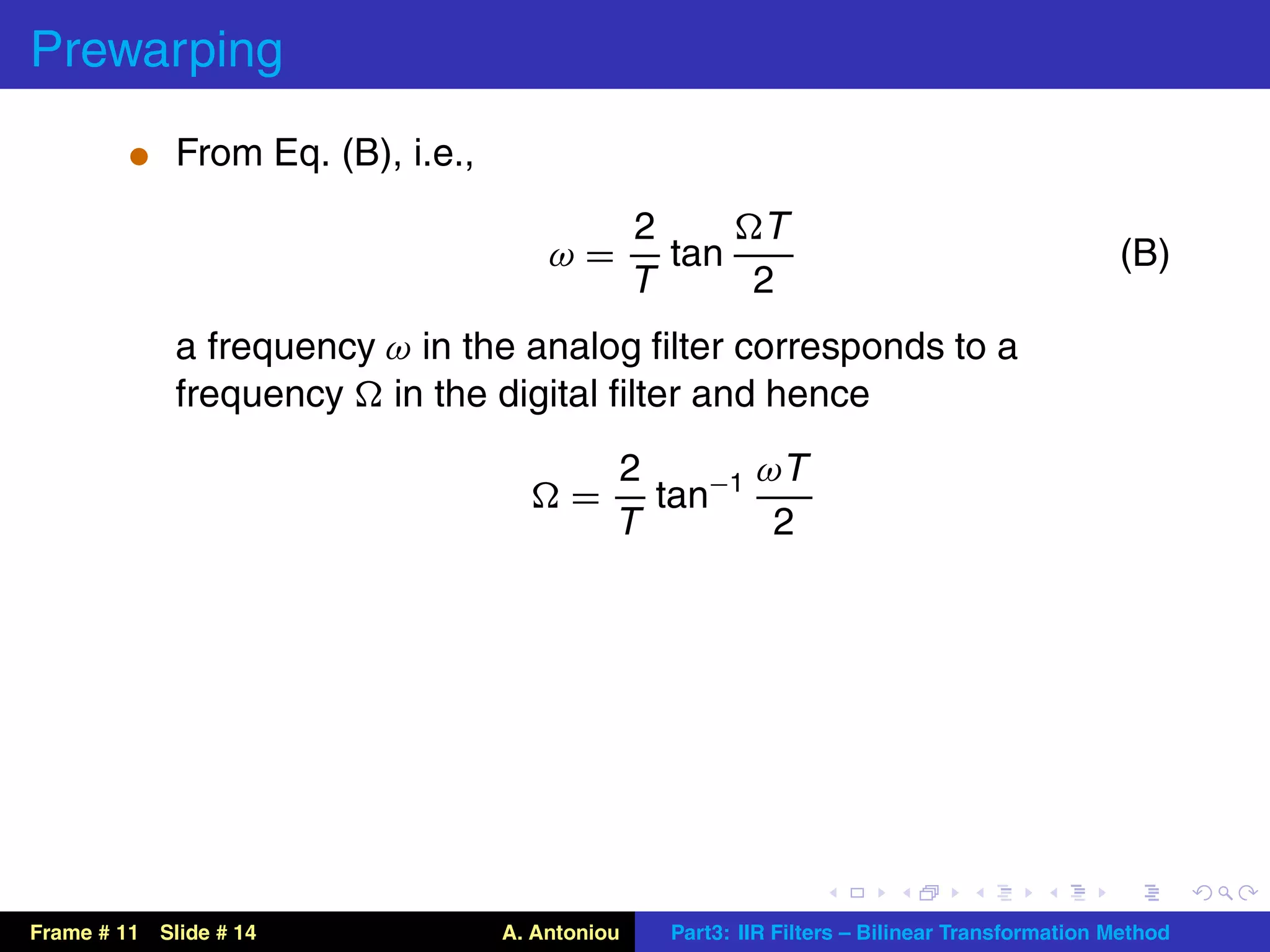

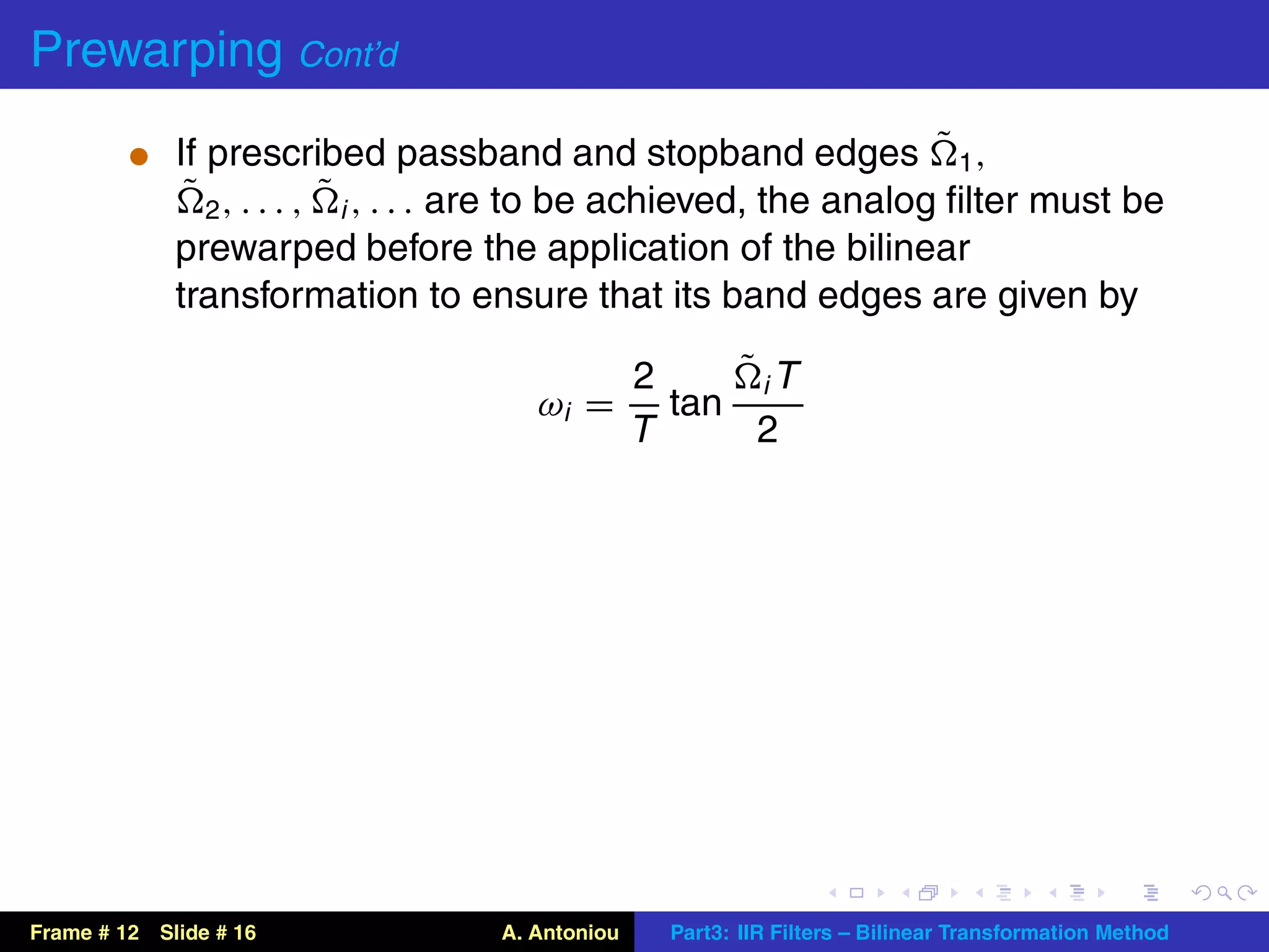
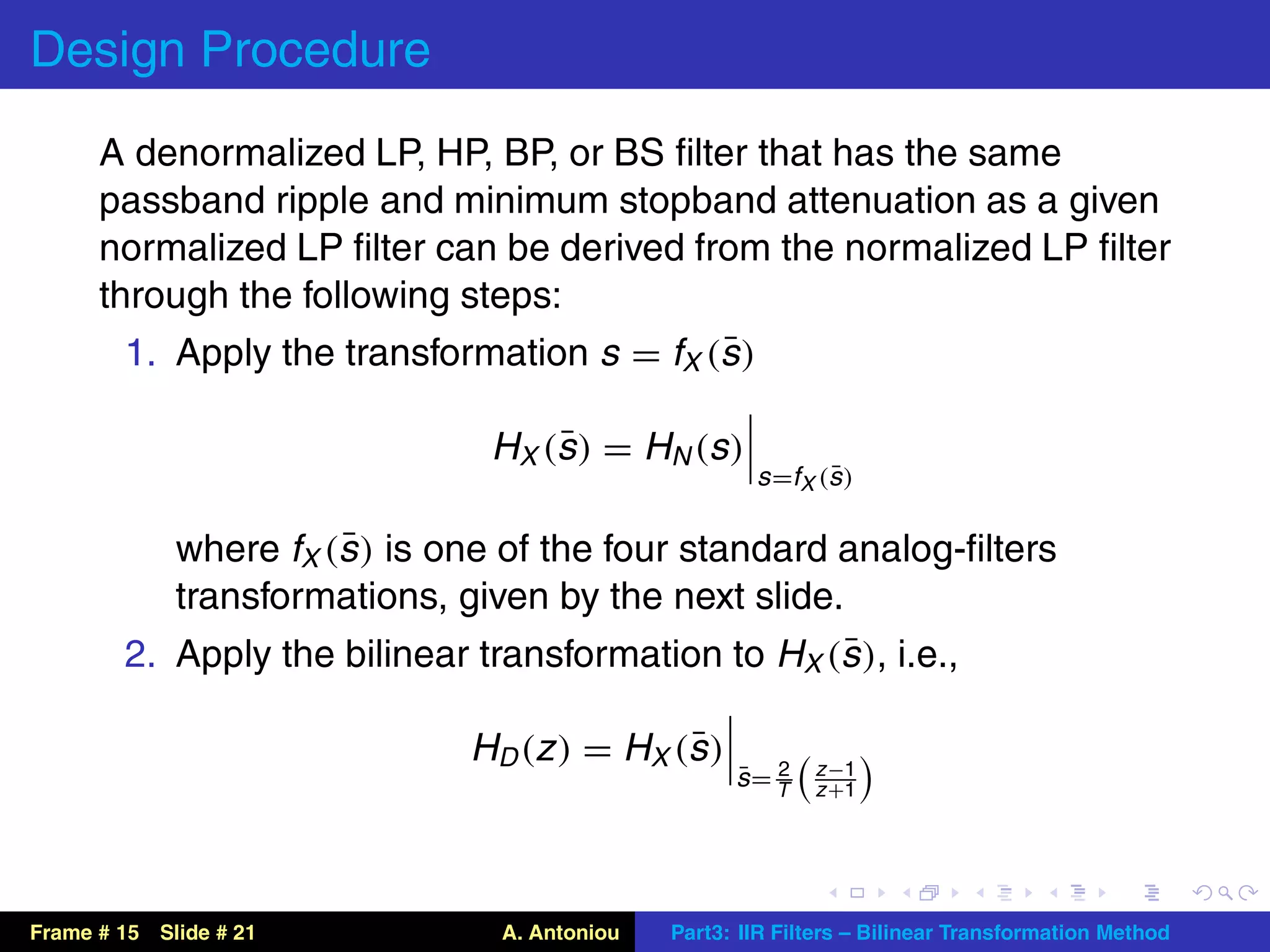
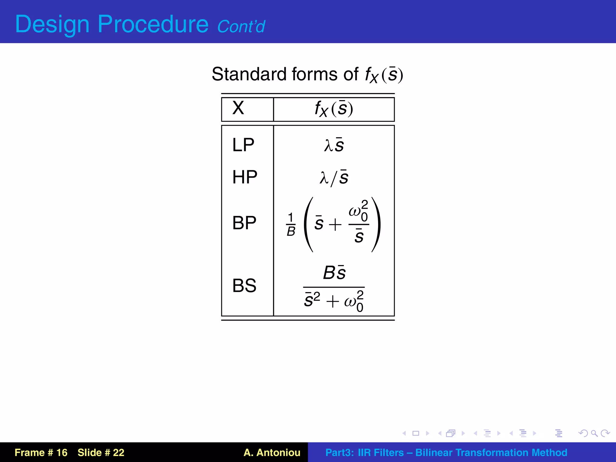

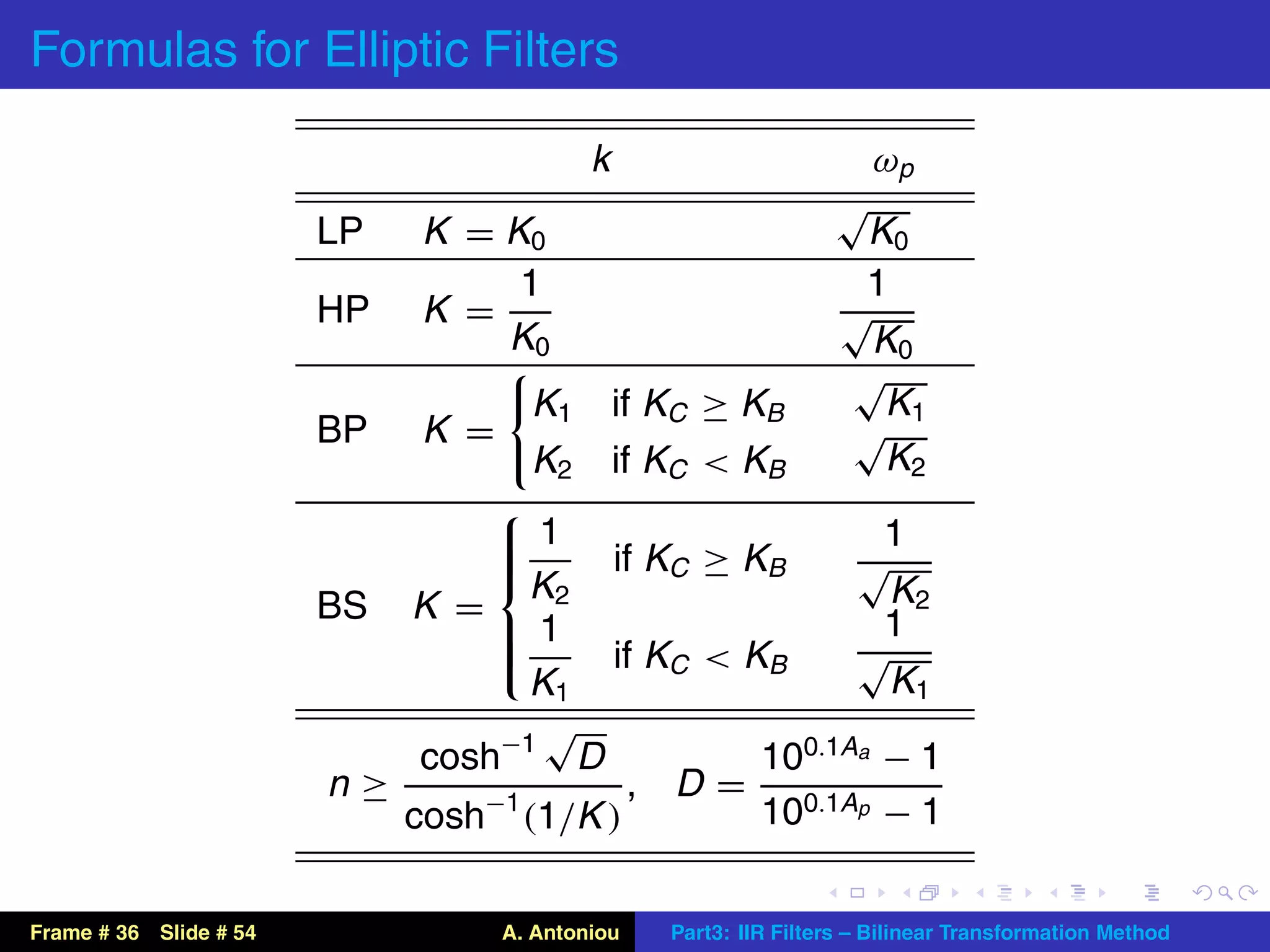


This document describes the bilinear transformation method for designing IIR filters. It begins by explaining that an analog filter design can be transformed into a digital filter design using the bilinear transformation. It then discusses the warping effect caused by this transformation at higher frequencies. To address this, the document presents the concept of prewarping analog filters so that the desired digital filter frequency responses are achieved after transformation. Finally, it outlines the general design procedure for lowpass filters using this method.