Download to read offline
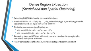
![Extracting Dense Regions From
HurricaneTrajectory Data[1]
Praveen KumarTripathi, Madhuri Debnath, Ramez Elmasri
Dept. of Computer Science, University ofTexas at Arlington
Presented By:
Vivek Kumar Sharma
[1]”GeoRich’14 Proceedings ofWorkshop on
Managing and Mining Enriched Geo-Spatial Data”](https://image.slidesharecdn.com/74a447f2-631b-4b01-ad42-31b883798f7d-151225061453/85/Paper2_CSE6331_Vivek_1001053883-1-320.jpg)
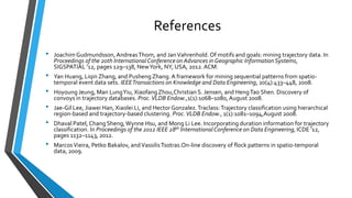
![Trajectory Clustering on Point Data
• Consider a trajectory as an individual Point
• Points are not constrained to belong to its respective parent trajectory or
sub-trajectory
[1] http://weather.unisys.com/hurricane/atlantic/2012H/index.php](https://image.slidesharecdn.com/74a447f2-631b-4b01-ad42-31b883798f7d-151225061453/85/Paper2_CSE6331_Vivek_1001053883-4-320.jpg)


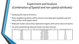
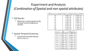
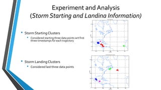


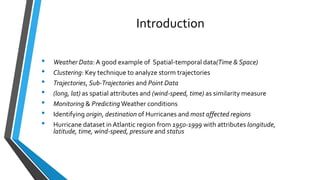
The document summarizes research on extracting dense regions from hurricane trajectory data using clustering techniques. It introduces DBSCAN clustering which identifies core points, border points, and outliers based on density. The researchers extend DBSCAN to cluster hurricane trajectory data points based on spatial attributes alone, and then combining spatial and non-spatial attributes like wind speed and time. Experiments analyze resulting clusters qualitatively and identify storm starting and landing regions. The work is compared to other trajectory clustering methods and concludes dense region extraction can provide insight into hurricane monitoring and prediction.