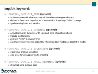
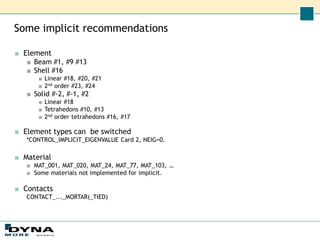
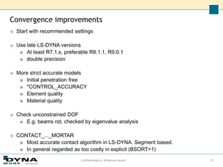
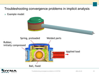
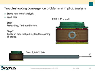
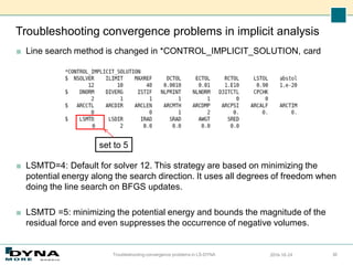
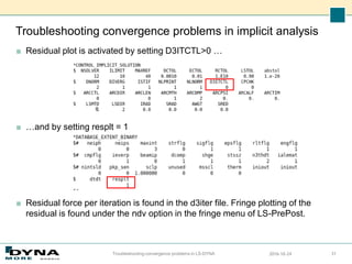
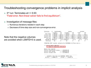
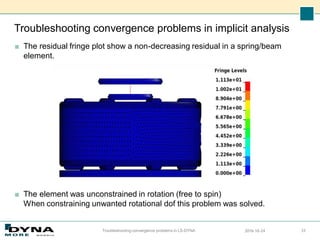
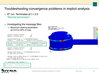
Overview, how to set up implicit analysis and improve convergence

Implicit analyses in LS-DYNA
Overview, how to set up implicit analysis
and improve convergence
Torbjörn Johansen, et al.
torbjorn.johansen@dynamore.se
DYNAmore Nordic Users Forum 2016, October 13-14
Workshop October 13 13.35-14.50

Outline
■ Introduction to implicit analysis
■ Implicit, how to set up
■ Convergence improvement
■ Example troubleshooting
■ Summary

Implicit Analysis Types
■ Nonlinear analysis
■ static or dynamic
■ Newton, Quasi-Newton, Arclength solution methods
■ Linear analysis
■ static or dynamic
■ single, multi-step
■ Eigenvalue based analysis
■ frequencies and mode shapes
■ linear buckling loads and modes
■ modal analysis: extraction and superposition
■ dynamic analysis by modal superposition
LS-DYNA Implicit, DYNAmore Nordic 3

■ Implicit
■ Iterative solution
■ Linearization necessary
■ Unconditionally stable
■ Few large time/load steps
■ Equilibrium! Convergence?
■ Structural static/dynamics:
■ Low frequency response, static
■ Vibration, oscillation
■ Strength, durability, NVH, …
■ Explicit
■ Direct solution
■ Decoupled: efficient, fast
■ Conditionally stable (Courant)
■ Many small time steps
■ Equilibrium? Energy balance!
■ Short time dynamics:
■ High frequency response
■ Wave propagation
■ Impact, crash, …
Explicit vs. Implicit
int
n
ext
n
n f
f
Ma 
 n
n
ext
n
n
n Ma
f
f
u
K
a
M 


 




int
1
1
1

Benefits with implicit analysis
■ Can be used to apply pre-loads (gravity, bolt pre-load) to a structure before
an explicit analysis.
■ Good for static and quasi-static problems. Time is not necessarily physical
time.
■ Frequency domain analysis (linear). Well suited for eigen-mode based linear
dynamics.
■ Time step size is in practice limited by:
■ Accuracy considerations,
frequency resolution, high frequency content in solution is lost.
■ Solvability of the system of nonlinear equations (automatic time step control is available).
■ Time step is not limited by any small and stiff elements, no mass scaling, as in explicit.
But …
■ More demanding when it comes to memory.
■ Check memory if simulation is not progressing, estimation in d3hsp.
■ Speed penalty for out-of-core solutions.
■ Harder to get normal termination, convergence of strong non-linear models.

General features
■ Fully nonlinear implicit solver
■ Large deformations
■ Contacts
■ Material non-linearity including failure
■ Static, dynamic or semi-dynamic
■ Implicit / explicit switching
■ Advanced solver technologies
■ Restart capabilities
■ Sub-modelling
■ Thermal solver - coupled or un-coupled
■ Wide range of elements, materials and constraints
■ Easy contact definition and powerful contact algorithm
6
LS-DYNA Implicit, DYNAmore Nordic

MPP Scalability
■ Performance – case study 900k element model
Blue curve = “ideal” scalability
Red curve = LS-DYNA MPP implicit
NCPUS
Speed

Non-linear implicit analysis
■ Maximum strength
Including material failure
■ Buckling analysis
■ Residual deformations
■ Roof crush

Frequency domain analysis
■ Frequency response function - FRF
*FREQUENCY_DOMAIN_FRF
Transfer functions for “unity” excitation
■ Steady state dynamics - SSD
*FREQUENCY_DOMAIN_SSD[_FATIGUE][_ERP]
Extension of FRF for frequency dependent excitation and binary plot, d3ssd.
Harmonic loading.
*MAT_ADD_FATIGUE Freq = 25 Hz

■ Random vibration
*FREQUENCY_DOMAIN_RANDOM_VIBRATION[_FATIGUE]
Uncertain loading, wind, wave, vibration …
Power Spectral Density, PSD, loading
Statistical response, 1 sigma.
Several methods for random
vibration fatigue available.
■ Response spectrum
*FREQUENCY_DOMAIN_RESPONSE_SPECTRUM
Maximum peak response analysis of structures.
Civil engineering, naval structures, etc.
Several mode combination methods, SRSS, NRL, CQC, …
Acceleration
PSD
(g^2/Hz)

■ Acoustics
*MAT_ACOUSTIC
■ *FREQUENCY_DOMAIN_ACOUSTIC_BEM[_OPTION]
_ATV
_MATV
_HALF_SPACE
_PANEL_CONTRIBUTION
■ *FREQUENCY_DOMAIN_ACOUSTIC_FEM
■ *FREQUENCY_DOMAIN_SEA[_OPTION]
_SUBSYSTEM
_CONNECTION
_INPUT_POWER

Outline
■Implicit, how to set up
■ Summary

Implicit keywords
■ *CONTROL_IMPLICIT_GENERAL (required for implicit)
■ activates implicit mode, explicit-implicit switching
■ defines implicit time step size
■ geometric stiffness activation
■ *CONTROL_IMPLICIT_SOLVER (optional)
■ parameters for and choice of linear equation solver,
which inverts stiffness matrix: [K]{x}={f}
■ controls extra output for debugging
■ *CONTROL_IMPLICIT_SOLUTION (optional)
■ parameters for nonlinear equation solver (Newton-based methods)
■ controls iterative equilibrium search
■ convergence tolerances
■ “linear" solution is selected here
■ controls extra output for debugging

Implicit keywords
■ *CONTROL_IMPLICIT_AUTO (optional)
■ activates automatic time step control (based on convergence history)
■ default is fixed time step size, error termination if any steps fail to converge
■ synchronizing loads and solution
■ *CONTROL_IMPLICIT_DYNAMICS (optional)
■ activates implicit dynamics with Newmark time integration scheme
■ include inertia terms
■ problem “time” is physical time
■ can improve convergence, especially when rigid body modes are present in model
■ *CONTROL_IMPLICIT_EIGENVALUE (optional)
■ eigenvalue analysis activation
■ also great for debugging/model checking
■ *CONTROL_IMPLICIT_MODAL_DYNAMICS (optional)
■ dynamics using a modal basis

Some implicit recommendations
■ Element
■ Beam #1, #9 #13
■ Shell #16
■ Linear #18, #20, #21
■ 2nd order #23, #24
■ Solid #-2, #-1, #2
■ Linear #18
■ Tetrahedons #10, #13
■ 2nd order tetrahedons #16, #17
■ Element types can be switched
*CONTROL_IMPLICIT_EIGENVALUE Card 2, NEIG=0.
■ Material
■ MAT_001, MAT_020, MAT_24, MAT_77, MAT_103, …
■ Some materials not implemented for implicit.
■ Contacts
CONTACT_..._MORTAR(_TIED)

Outline
■Convergence improvement
■ Summary

Convergence improvements
■ Start with recommended settings
■ Use late LS-DYNA versions
■ At least R7.1.x, preferable R8.1.1, R9.0.1
■ double precision
■ More strict accurate models
■ Initial penetration free
■ *CONTROL_ACCURACY
■ Element quality
■ Material quality
■ Check unconstrained DOF
■ E.g. beams rot, checked by eigenvalue analysis
■ CONTACT_..._MORTAR
■ Most accurate contact algorithm in LS-DYNA. Segment based.
■ In general regarded as too costly in explicit (BSORT=1)

■ Activate more output for convergence debugging
■ LPRINT, NLPRINT, RESPLT, D3ITCTL
■ Time step size
■ Too large step may inhibit convergence.
■ Too small may lead to long simulation times. Use automatic time step
option.
■ Full Newton for strong non-linear problems
■ ILIMIT=1, new stiffness matrix reformation every iteration
■ Turn on dynamics
■ Include inertia effects before any contacts are established
■ Ramp down dynamic effects if static analysis

■ First step – basic model checking ...
■ Check mesh quality, avoid “4-noded trias” poorly shaped “pentas”
■ Negative / small volume for 2nd order tets
■ Poor aspect ratio of elements
■ Avoid CNRBs with common nodes
■ Check material data, slopes of hardening curves
■ Consistency of unit system
2014-09-09
Troubleshooting convergence problems in LS-DYNA 19

Procedures for solving convergence problems
■ Try to determine the reason
examine error and warning messages in d3hsp and messag (mes00XX) files.
■ Activate print flags to get more information.
■ View deformed geometry during iteration process using "d3iter" database to
isolate problem areas.
■ Request output of residual force by setting RESPLT=1 on
*DATABASE_EXTENT_BINARY.
■ Carefully inspect input deck
■ Check smoothness of curves
■ Check material properties
■ Check contact penetrations, remove if found
■ Check magnitude of loads / unit system
■ Check contacts, make sure soft part is slave
■ Check elements, avoid small Jacobians and distorted elements
2014-09-09

Convergence improvements tips and tricks
■ Switch to full Newton
(ILIMIT=1 on *CONTROL_IMPLICIT_SOLUTION)
■ Turn on dynamics if simulation is static (*CONTROL_IMPLICIT_DYNAMICS)
■ Recommended initially for assemblies with “loose” parts that are to be
clamped together by for example bolted joints
■ If too much dynamics, increase simulation time or reduce densities
■ Decrease (maximum) time step
■ Switch to _TIED – contacts in order to identify which contact is causing
problems
■ Decrease contact stiffness. Observe penetrations.
■ Experiment with geometric stiffness
(IGS on *CONTROL_IMPLICIT_GENERAL)
■ Switch to elastic materials
■ If large displacements, change DNORM to 1 and increase DCTOL
■ Try switching to displacement controlled loading if possible
■ For soft materials, use fully integrated elements or increase hourglass
stiffness
2014-09-09

Convergence improvements tips and tricks
■ Do an eigenvalue analysis initially and intermittent
■ Reveals rigid body modes that are not constrained – “loose” parts
■ Reveals beams that can spin about their axis
■ Reveals truss and spring elements that are inproperly modelled
■ Observe convergence progress of displacement, energy norms
(view d3hsp file or activate NLPRINT flag for screen output)
■ If tolerances nearly satisfied
■ Allow a few more iterations
■ Experiment with slightly relaxed convergence tolerance (make sure you
are content with the model first)
■ (Interactively force convergence using “<ctrl-c> converge“ and see what
happens ...)
2014-09-09

Outline
■Example troubleshooting
■ Summary

Troubleshooting convergence problems in implicit analysis
■ Example model
2016-10-24
Ball, fixed
Welded parts
Applied load
Spring, preloaded
Rubber,
initially compressed

■ Static non-linear analysis
■ Load case
Step 1
Preloading, find equilibrium.
Step 2
Apply an external pulling load/unloading
of 350 N.
2016-10-24
Step 1, t= 0-0.2s
Step 2, t=0.2-2.0s
F

■ 1st run: Terminates after initiating:
“Fatal error. Non-linear solver fails to find equilibrium”.
■ Investigation of message files:
■ Negative volume failure
2016-10-24

2016-10-24

■ LS-PrePost, Model checking, shows initial penetrations in contacts.
■ Actions:
■ Set parameter IGNORE = 1 to handle initial penetrations.
■ Set NLPRINT = 3 for more Newton solver information.
■ IGNORE is found in *CONTACT_..._MORTAR optional card C.
0 Default to control contact
1, 2 Allow initial penetrations, warning output
3, 4 Remove initial penetrations in time MPAR1 (Only Mortar)
■ NLPRINT is found in *CONTROL_IMPLICIT_SOLUTION, card 2.
0 no information
1 print iteration information
2 extra information of solver status at each iteration
3 as 2 and additional information at each line search step
2016-10-24

■ 2nd run: Terminates at t = 0.85
■ Numerous iteration are needed
■ Negative eigenvalues
■ Negative volume failure
■ Actions:
■ Choose line search method 5
(LSMTD=5)
■ Activate residual plot
2016-10-24
…..
…..

■ Line search method is changed in *CONTROL_IMPLICIT_SOLUTION, card
■ LSMTD=4: Default for solver 12. This strategy are based on minimizing the
potential energy along the search direction. It uses all degrees of freedom when
doing the line search on BFGS updates.
■ LSMTD =5: minimizing the potential energy and bounds the magnitude of the
residual force and even suppresses the occurrence of negative volumes.
2016-10-24
set to 5

■ Residual plot is activated by setting D3ITCTL>0 …
■ …and by setting resplt = 1
■ Residual force per iteration is found in the d3iter file. Fringe plotting of the
residual is found under the ndv option in the fringe menu of LS-PrePost.
2016-10-24

■ 3rd run: Terminates at t = 0.93
■ Numerous iterations needed in each step
■ Decrease of time step size and non-convergence error.
Note that the negative volumes
are avoided when LSMTD=5 is used.
2016-10-24

■ The residual fringe plot show a non-decreasing residual in a spring/beam
element.
■ The element was unconstrained in rotation (free to spin)
When constraining unwanted rotational dof this problem was solved.
2016-10-24

■ 4th run: Terminates at t = 1.11
■ Numerous iterations needed
in each step
■ Decrease of time step size and
non-convergence error.
■ Energy norm ratio < ECTOL
■ Decreasing residual norm
■ Displacement norm ratio
is oscillating
=> Slow convergence!
2016-10-24
ECTOL=0.01
DCTOL=0.001

■ Investigation of model show:
■ Critical contact penetrations
■ Actions:
■ Turn on contact status output. MINFO = 1 on *CONTROL_OUTPUT
2016-10-24
Close to critical penetration depth?
Cross section

■ Investigating the message files:
■ Failed contact
■ Critical penetrations (~100%)
in converged steps.
■ The contacts will probably fail
in the next step.
2016-10-24

■ Actions:
■ Increase contact thickness (not desired, not used)
■ Increase penalty stiffness factor (increased from 1.0 to 2.0)
■ Increase maximum allowable contact force up to critical penetration (IGAP is set to 10)
2016-10-24
Increasing IGAP may slow
convergence.

“Normal termination”.
■ Investigating the message files:
■ Maximum relative penetration
at t=2.0 is 24% of max
2016-10-24

Outline
■Summary

LS-DYNA Implicit objectives
■ To provide a complete implicit solver, fully comparable to any other implicit
code when it comes to functionality, robustness and performance.
■ Full integration in the LS-DYNA code, making it easy to take advantage also of
the well-established explicit solver’s features.
■ Make it easier to share models between disciplines, for example crash and
fatigue or NVH.
2014-09-09

Summary
■ Implicit functionality, both nonlinear and linear, is implemented in LS-
DYNA.
■ Efficiently parallelized code, MPP and SMP.
■ Licenses (all features) already on site.
■ Customer requests for improved functionality is encouraged to
motivate further development.

Knowledge resources
■ Guidelines
■ LS-DYNA implicit guidelines package (recommendations, control cards, etc)
■ Relevant training seminars (www.dynamore.se)
■ Introduction to LS-DYNA (3 days)
■ LS-DYNA Implicit Analysis (3 days)
■ Getting started with Non-linear Implicit Analysis in LS-DYNA (1 day)
■ NVH & Frequency Domain Analysis in LS DYNA (2 days)
■ Webinairs (1 hour)
■ Support sites
■ www.dynasupport.com
■ www.dynaexamples.com
■ www.dynalook.com
■ Support
■ support@dynamore.se

Thank you!
Your LS-DYNA distributor and
more

Overview, how to set up implicit analysis and improve convergence

More Related Content

Recently uploaded

Featured

Overview, how to set up implicit analysis and improve convergence