1. Optimum Time Series Granularity in the Estimation of Financial Beta
Manuel G. Russon, Ph.D.
St. John’s University
Qiaochu Geng
St. John’s University
Abstract
In the worldof finance andportfoliomanagement,“beta”referstothe sensitivityof a security’sreturn
to the sensitivityof the “market”portfolioandisanindicationof the level of systematicrisk,i.e.the
amountof riskthat a company’sequityshareswiththe entire market. Correctvaluesforbetaare
crucial for portfoliomanagers, asthe clientcontractalmostalwayscallsfora portfoliobetaequal to1.0.
Typically,betaisestimatedusingOrdinaryLeastSquareswithmonthlygranularity. Thisresearch
considersthatthe ideal granularitymightbe somethingotherthanmonthly. Betasforall companiesin
the SP500 are estimatedwithdaily,monthly, quarterlyand yeargranularity. Optimumgranularityis
determinedtobe quarterly.
I. Introduction
In the worldof finance andportfoliomanagement,“beta”referstothe sensitivityof asecurity’sreturn
to the sensitivityof the “market”portfolioand isanindicationof the level of systematicrisk,i.e.the
amountof riskthat a company’sequityshareswiththe entire market.
Mathematically,betaisthe regression slope inalinearregressionof companyrate of returnonto the
marketrate of return. Eqn. 1, below,isthe equationforbetaandisreferredtoasthe characteristicline.
rri = +*rrmkt (1)
Where rri - rate of returnfor companyi
rrmkt - rate of return formarket
 - alpha,intercept
 - beta,slope
The intercept, ,isthe expectedreturnwhenthe marketreturnisequal to0 and the slope, ,isthe
percentchange inthe securityfora one percentchange inthe marketreturn,on average otherthings
equal.

2. The conventional methodtoestimatethe characteristicline alphaandbetais OLS,i.e. ordinaryleast
squaresusingmonthlyobservations. Thisresearchestimatesbetafor4 levelsof granularity,i.e.daily,
monthly,quarterly,andyearlytofindthe optimumlevel of granularity.
Correct estimationof betaisimportantfromanassetmanagement,managerial finance and/oran
investmentbankingperspective. Fromanassetmanagementperspective,the followingconstraintsare
imposeduponportfoliomanagers:
1. PortfolioTurnover- usuallylimitedto100% peryear
2. Numberof namesinportfolio -usuallyrequiredtobe 50 – 100
3. TrackingError - usuallylimitedtobe +- 3% of index
4. WeightedAve.Beta- usuallyconstrainedto.98-1.02
All of these constraintsare imposedtopreventexcessiverisktakingbythe portfoliomanager. Inthe
case of item4, incorrectbetascan leadto unexpectedvolatilitywithconcomitantissuesinportfolio
managementregardingitems1-3. Institutional assetmanagersrelyonbetasprovidedbyvendorssuch
as Barra or Bloomberg. Buteventhese vendorsneedtobe sure theirbetasaccuratelyreflectreality.
An individual retailinvestorcanassessthe expectedvolatilityof the company’sequityrelativetoa
universe benchmarkbylookingupabeta onYahoo/Finance orotherfree source. Ina more formal,
institutional assetmanagementcontext,portfoliomanager of institutionalclients,e.g.foundations,
pensionfunds,mutual funds,etc.mustsatisfyanumberof constraintsintheirportfoliomanagement
activities.
In a capital budgetingcontext,accurate betasare neededforestimationof costof capital. An
inaccurate betageneratesinaccurate costof capital,and thiscouldleadtothe incorrectacceptance or
rejectionof acapital project.
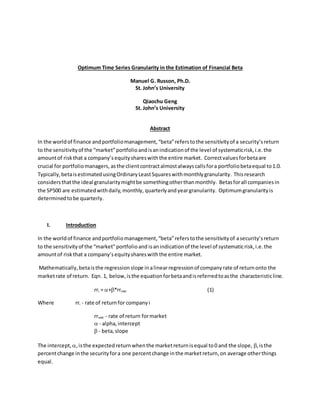
Figs.1-4 displayscatter-plotsof rate of returnforCaterpillar,Inc. vs.rate of returnfor SP500 for four
levelsof time seriesgranularitywithlinearmodelplotsoverlaid. Betaisthe slope of the linearmodel.
The questiontobe addressedinthisresearchisthe appropriate levelof granularitytodiscoverthe
appropriate beta.

3. Fig.1 Yearly Return-SP500 Vs.CAT
rr SP500
rrCAT
-0.4 -0.2 0.0 0.2
-0.40.00.40.8
Fig.2 Quarterly Return-SP500 Vs.CAT
rr SP500
rrCAT
-0.3 -0.2 -0.1 0.0 0.1 0.2
-0.40.00.20.4
Fig.3 Monthly Return-SP500 Vs.CAT
rrSP500
rrCAT
-0.15 -0.10 -0.05 0.0 0.05 0.10
-0.20.00.2
Fig.4 Daily Return-SP500 Vs.CAT
rr SP500
rrCAT
-0.05 0.0 0.05 0.10
-0.15-0.050.050.15
II. Methodology
End of day, month,quarterand yearclosingpricesforall SP500 constituentsasof 12/31/2015 were
downloadedfromBloomberg forthe period 12/31/1980-12/31/2016. As some companiesare newerto
the index,theyhave fewerdatapointsthanothers. Returnswill be calculatedandbetacoefficients
estimatedforeachcompany foreach time series granularity.Graphical (histogramsandscatterplots)
and analytical techniques(descriptive statistics,correlationandregressionwill be usedtodetermine
optimumgranularity. The datawill be estimatedusingS+.

4. Eqns.2, 3, and 4 displaythe functionalspecification,populationregression lineandsample regression
line inthe estimationof beta.
+
Eqn. 2 rri= f(rrmkt) (2)
Eqn. 3 rri = +*rrmkt (3)
Eqn. 4 rri = a+b*rrmkt (4)
III. Results
A histogramof all betasappearsinFigs.1-4, and pairs scatter-plotsappearinFigs.5. The betaresults of
all 500 companiesare containedinAppendix1.
Figs.5-8 Histograms of Beta Coefficients
-2 0 2 4
050100150
Fig.5 Histogram of Yearly Beta
betaR es ults 1$betay
0.0 0.5 1.0 1.5 2.0
0204060
Fig.6 Histogram of Montly Beta
betaR es ults 1$betam
0.0 0.5 1.0 1.5 2.0
0204060
Fig.7 Histogram of Quarterly Beta
betaR es ults 1$betam
0.5 1.0 1.5 2.0
020406080100
Fig.8 Histogram of Daily Beta
betaR es ults 1$betad
Table 1 displaysbetacoefficientsforregressionsfromtenlarge companies,asubsetof the resultof time
seriesregressionsforall SP500 constituents.
Table 1 Beta Coefficientsfor10 Companies
tkr betay betaq betam betad
15 aapl. 1.70 1.43 1.49 1.12
46 amzn. 1.74 1.25 1.49 1.30
134 dd. 0.99 1.20 1.29 1.02
153 duk. 0.76 0.53 0.47 0.56
261 jnj. 0.34 0.35 0.42 0.52
439 t. 0.63 0.52 0.59 0.78
473 utx. 1.02 1.09 0.94 0.97
490 wfc. 0.46 1.04 0.92 1.32
496 wmt. 0.03 0.28 0.36 0.65
506 xom. 0.43 0.70 0.57 0.85
Table 2 and3 displaydescriptive statisticsandcorrelationmatrixforthe betascontainedinAppendix1.
Table 2 Descriptive Statistics for Beta Estimates of 500 Companies

5. mean med stdev skew kurt n
betay 1.08 0.99 0.69 1.21 4.23 514
betaq 1.07 1.01 0.52 0.73 0.77 514
betam 1.04 1.01 0.48 0.40 -0.33 514
betad 1.03 1.04 0.31 0.20 -0.24 514
Table 3 CorrrelationMatrix for Beta Estimates of 4 Granularities
betay betaq betam betad
betay 1.00 0.71 0.70 0.59
betaq 0.71 1.00 0.91 0.79
betam 0.70 0.91 1.00 0.87
betad 0.59 0.79 0.87 1.00
Fig.9 displaysscatterplotpairsof the betaestimatescontainedinAppendix1.
Fig. 9 Scatterplot Pairs
betay
0 1 2 3 0.5 1.0 1.5 2.0
-201234
0123
betaq
betam
0.01.02.0
-2 -1 0 1 2 3 4
0.51.01.52.0
0.0 0.5 1.0 1.5 2.0
betad
A lotin the wayof diagnosticsispresented. The determinationof which granularitymustbe made on
the basisof these diagnostics. We findmonthlybetatobe mostcompellingonthe basisthatthe mean
and medianare 1.04 and 1.01, bothmost nearto 1.0.
Conclusion
Thisresearch evaluated betaestimateswithfourgranularitiestodetermine optimumgranularityinthe
estimationof financialbeta. Optimumgranularitywasdeterminedtobe monthly. Furtherresearchis
neededforamore conclusive determination.