This document introduces the authors and contributors of the textbook "Operating Systems: Concepts with Java". It provides brief biographies of Abraham Silberschatz, Peter Baer Galvin, and Greg Gagne, describing their academic and professional backgrounds. It then summarizes the organization and goals of the textbook, which aims to clearly describe fundamental operating systems concepts through examples from commercial systems like Solaris, Linux, Windows, and Mac OS X. The textbook is organized into nine parts covering topics like processes, memory management, storage, protection, and distributed systems.
![xiv
Joseph Boykin, Jeff Brumfield, Gael Buckley, Roy Campbell, P. C. Capon, John
Carpenter, Gil Carrick, Thomas Casavant, Bart Childs, Ajoy Kum.ar Datta,
Joe Deck, Sudarshan K. Dhall, Thomas Doeppner, Caleb Drake, M. Racsit
Eskicioglu, Hans Flack, Robert Fowler, G. Scott Graham, Richard Guy, Max
Hailperin, Rebecca I-Iartncan, Wayne Hathaway, Christopher Haynes, Don
Heller, Bruce Hillyer, Mark Holliday, Dean Hougen, Michael Huangs, Ahmed
Kamet Marty Kewstet Richard Kieburtz, Carol Kroll, Marty Kwestet Thomas
LeBlanc, John Leggett, Jerrold Leichter, Ted Leung, Gary Lippman, Carolyn
Miller, Michael Molloy, Euripides Montagne, Yoichi Muraoka, Jim M. Ng,
Banu Ozden, Ed Posnak, Boris Putanec, Charles Qualline, John Quarterman,
Mike Reiter, Gustavo Rodriguez-Rivera, Carolyn J. C. Schauble, Thomas P.
Skimcer, Yannis Smaragdakis, Jesse St. Laurent, John Stankovic, Adam Stauffer,
Steven Stepanek, John Sterling, Hal Stern, Louis Stevens, Pete Thomas, David
Umbaugh, Steve Vinoski, Tommy Wagner, Larry L. Wear, Jolm Werth, James
M. Westall, J. S. Weston, and Yang Xiang
Parts of Chapter 12 were derived from a paper by Hillyer and Silberschatz
[1996]. Parts of Chapter 17were derived from a paper by Levy and Silberschatz
[1990]. Chapter 21 was derived from an unpublished manuscript by Stephen
Tweedie. Chapter 22 was derived from an unpublished manuscript by Dave
Probert, Cliff Martin, and Avi Silberschatz. Appendix C was derived from
an unpublished manuscript by Cliff Martin. Cliff Martin also helped with
updating the UNIX appendix to cover FreeBSD. Some of the exercises and
accompanying solutions were supplied by Arvind Krishnamurthy.
Mike Shapiro, Bryan Cantrill, and Jim Mauro answered several Solaris-
related questions. Bryan Cantrill from Sun Microsystems helped with the ZFS
coverage. Steve Robbins of the University of Texas at San Antonio designed
the set of simulators that we incorporate in WileyPLUS. Reece Newman
of Westminster College initially explored this set of simulators and their
appropriateness for this text. Josh Dees and Rob Reynolds contributed coverage
of Microsoft's .NET. The project for POSIX message queues was contributed by
John Trona of Saint Michael's College in Colchester, Vermont.
Marilyn Turnamian helped generate figures and presentation slides. Mark
Wogahn has made sure that the software to produce the book (e.g., Latex
macros, fonts) works properly.
Our Associate Publisher, Dan Sayre, provided expert guidance as we
prepared this edition. He was assisted by Carolyn Weisman, who managed
many details of this project smoothly. The Senior Production Editor Ken
Santor, was instrumental in handling all the production details. Lauren Sapira
and Cindy Jolmson have been very helpful with getting material ready and
available for WileyPlus.
Beverly Peavler copy-edited the manuscript. The freelance proofreader was
Katrina Avery; the freelance indexer was WordCo, Inc.
Abraham Silberschatz, New Haven, CT, 2008
Peter Baer Galvin, Burlington, MA 2008
Greg Gagne, Salt Lake City, UT, 2008](https://image.slidesharecdn.com/elecnwintjql7eggtsqw-operating-system-concepts-8th-editiona4-230117160154-4fa44b38/85/Operating_System_Concepts_8th_EditionA4-pdf-12-320.jpg)

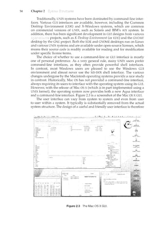
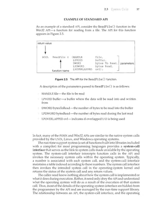
![1.2
THE STUDY OFOPERATING SYSTEMS
Therehas neverbeenarnore interestirighnwtostudyoperatingsystems:·and
ithas neverb.een.e~sier.Theopen-sourc;e movernent has overtaken.operating
systems, caJ.tsing marlyofthenctobemadeavailable inbothsourceand binary
(e~ecuta]Jle) fonnat.·.This Iistindud~~Linu)(, BSDUNIX/Solat•is,and part of•
]II~cos.x. Th~availa~ilityqf·source.code.q,llowsus.tostudyoperq,til}.gsy?tems
frorrt theinsid,eout' ..Questionsthat previo)1sly could onlyb~ answerecL~y
lookingatdocumentaticmor thebehayior.ofan op~rating systemc.annow be
answered byexamining the codeitself.
In additi?n,.therise of virtualization as a ll}.ainsfreafll. (andfrequelltlyfree)
cmnp)1ter ftmctionmakesitpos;~i1Jlet()runnmnyoperqtingsystems.ontop.of
onecoresystem..Forexample,VMware(J:lttp.://www .•vmwarE:).com):provides
afree·''player'' onwhich hundreds.of free .''virtualappliilnces'' cann.m.Using
this method,students call tryolit hundreds.ofoperatingsystems.withintheir
existing operatingsystems .atno cost. ...··. ... .·. ·.. ·...·
Operating .sy~temsthat are no lortge~ ~ofllmerci~lly viableltave been
opell-~o}lrced asvvell, ·enablirtg·.usto study how system~ pperated i~<
time.of•.•f~v.r~r CPU, ll}.emory,•·•etnd.storcrge•·•·.resoJ.trces,·····.An...exten~iye.b).It·•not
complete.•.list ()f 9pen'-sourct operafirtg-"system pr?j~?ts is..availa~le £rom
ht~p ://dm()~ ' org/C:omp)1ters/Softp(lre/Operati»g:-Systems/p~~m._Sourc~/-
S.i.m
..•..•·..·.u.l·a·t·o
..rs.•·..o··.f······s··..P
...e
...c
..i.fi
..·.·c··
..··. ·•.h
.....a
...·.r
...·.d
...•w
...•·.a.•.r
...e
.....·.·....ar..e·
... ·.a·l·s·o
..·......a·.··v
...•·...a.il
..·<1.b
...·.·.le··
...·.i·n···.·
..·
...·...s
..om
.•.·. ·..e. •.·.c.·.·....a····.·s·e·s.'····...al..I.·.o
.......w.·
.•..m.·
.•··.g
..
th~ operat~<g systell}.to.runon.''na~ve''.hardware, ...all~ithrrtthec?l}.fines
of a modem CO!TIPJ-Iter and moderJ1 OPf/'atirtg ~ystem. For: example, a
DECSYSTEMc20 simulator running on Mac OS Xcan boot TOPS-20, loa~. the
~ource.tages;.·and modify al'ld comp~le·<l·.J:t.evvTOPS-20 .k~rneL ··Art·interested
stltdent ~ar• search theint~rnet to find the origillal papers that de~cribe the
operating systemand..the.origipa~ manuals:
Tl<e adve~t?fogen-source operafirtg sy~te1Tis also l}."lal<es it easyt?··.make
the move fromstu~enttooper<:lting~systemdeveloper.With some knov.rledge,
som~ effo1't, a11d an Internet connection,a student c;al'leven create a new
operating-systemdistribution! Justa. fev.r years, ~go itwas diffic]_llt or
if1Lpossible ··to. get acce~s·. to ·source co?e. .N?v.r·.that access is.·liJnited only
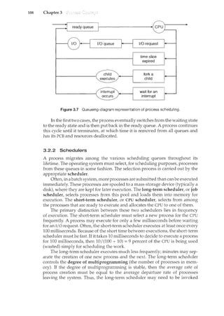
bylt()wmuchtimeand disk spacea student has. ·
7
with computer-system organization, so you can skim or skip it if you already
understand the concepts.
1.2.1 Computer-System Operation
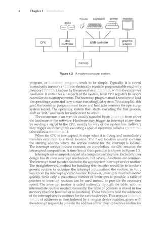
A modern general-purpose computer system consists of one or more CPUs
and a number of device controllers connected through a common bus that
provides access to shared memory (Figure 1.2). Each device controller is in
charge of a specific type of device (for example, disk drives, audio devices, and
video displays). The CPU and the device controllers can execute concurrently,
competing for memory cycles. To ensure orderly access to the shared memory,
a memory controller is provided whose function is to synchronize access to the
memory.
For a computer to start rum<ing-for instance, when it is powered
up or rebooted-it needs to have an initial program to run. This initial](https://image.slidesharecdn.com/elecnwintjql7eggtsqw-operating-system-concepts-8th-editiona4-230117160154-4fa44b38/85/Operating_System_Concepts_8th_EditionA4-pdf-25-320.jpg)
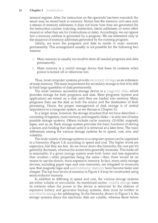
![CPU user
1/0
device
process
executing
1/0 interrupt
processing
idle "~""~-~-
tmcefeniog I L
..
1/0
request
1.2
ll v
-~~'"''''''~'"''"-~~ -~~-"] t---~---
''m'] L,~"~~~
transfer
done
1/0 transfer
request done
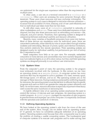
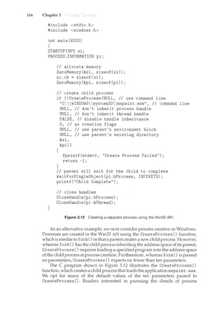
Figure 1.3 Interrupt time line for a single process doing output.
9
the interrupting device. Operating systems as different as Windows and UNIX
dispatch interrupts in this manner.
The interrupt architecture must also save the address of the interrupted
instruction. Many old designs simply stored the interrupt address in a
fixed location or in a location indexed by the device number. More recent
architectures store the return address on the system stack. If the interrupt
routine needs to modify the processor state-for instance, by modifying
register values-it must explicitly save the current state and then restore that
state before returning. After the interrupt is serviced, the saved return address
is loaded into the program counter, and the interrupted computation resumes
as though the interrupt had not occurred.
1.2.2 Storage Structure
The CPU can load instructions only from memory, so any programs to run must
be stored there. General-purpose computers run most of their programs from
rewriteable memory, called main memory (also called
or RAM). Main commonly is implemented in a semiconductor
technology called Computers use
other forms of memory as well. Because the read-only memory (ROM) camwt
be changed, only static programs are stored there. The immutability of ROM
is of use in game cartridges. EEPROM camwt be changed frequently and so
contains mostly static programs. For example, smartphones have EEPROM to
store their factory-il<stalled programs.
All forms of memory provide an array of words. Each word has its
own address. Interaction is achieved through a sequence of load or store
instructions to specific memory addresses. The load instruction moves a word
from main memory to an internal register within the CPU, whereas the store
instruction moves the content of a register to main memory. Aside from explicit
loads and stores, the CPU automatically loads instructions from main memory
for execution.
A typical instruction-execution cycle, as executed on a system with a
architecture, first fetches an il1struction from memory and stores
that instruction in the . The instruction is then decoded
and may cause operands to be fetched from memory and stored in some](https://image.slidesharecdn.com/elecnwintjql7eggtsqw-operating-system-concepts-8th-editiona4-230117160154-4fa44b38/85/Operating_System_Concepts_8th_EditionA4-pdf-27-320.jpg)
![1.4 19
Figure 1.9 Memory layout for a multiprogramming system.
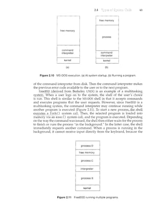
!()_C()_tnpl~te: In a non-multiprogrammed system, the CPU would sit idle. In
a multiprogrammed system, the operatilcg system simply switches to, and
executes, another job. When that job needs to wait, the CPU is switched to
another job, and so on. Eventually the first job finishes waiting and gets the
CPU back. As long as at least one job needs to execute, the CPU is never idle.
This idea is common in other life situations. A lawyer does not work for
only one client at a time, for example. While one case is waiting to go to trial
or have papers typed, the lawyer can work on another case. If he has enough
clients, the lawyer will never be idle for lack of work. (Idle lawyers tend to
become politicians, so there is a certain social value in keeping lawyers busy.)
Multiprogrammed systems provide an environment in which the various
system resources (for example, CPU, memory, and peripheral devices) are
utilized effectively, but they do not provide for user interaction with the
computer system. is_~l()gi~alex_tension of
multiprogramming. ~' time-s!caring syste~s,the CPl] execu~eslnl1ltiplejobs
by switcll.Ing~ainong them, but the switches occur so frequently that the ~1sers
canh~teract with eachprograffi~vEre l.t1sil.mning.--····
-Ti1ne shar:il~g requi.i-es an .. (or -
which provides direct communication between the user and the system. The
user gives instructions to the operating system or to a program directly, using a
input device such as a keyboard or a mouse, and waits for immediate results on
an output device. Accordingly, !!'te sho~1ld be sh()rt=typically
less than one second.
A time-shared operating system allows many users to share the computer
simultaneously. Since each action or command in a time-shared system tends
to be short, only a little CPU time is needed for each user. As the system switches
rapidly from one user to the next, each user is given the impression that the
entire computer system is dedicated to his use, even though it is being shared
among many users.
A time-shared operating system 11ses CPU scheduling and multiprogram-
ming to provide each user with a small portion of a time-shared computer.
Eachuserhas atleast or:t_e S§parateprogra111inmemory. A program loaded into](https://image.slidesharecdn.com/elecnwintjql7eggtsqw-operating-system-concepts-8th-editiona4-230117160154-4fa44b38/85/Operating_System_Concepts_8th_EditionA4-pdf-33-320.jpg)
![1.5 21
be performed. The interrupt-driven nature of an operating system defines
that system's general structure. For each type of interrupt, separate segments
of code in the operating system determine what action should be taken. An
interrupt service routine is provided that is responsible for dealing with the
interrupt.
Since the operating system and the users share the hardware and software
resources of the computer system, we need to make sure that an error in a
user program could cause problems only for the one program running. With
sharing, many processes could be adversely affected by a bug in one program.
For example, if a process gets stuck in an infinite loop, this loop could prev.ent
the correct operation of many other processes. More subtle errors can occur
in a multiprogramming system, where one erroneous program might modify
another program, the data of another program, or even the operating system
itself.
Without protection against these sorts of errors, either the computer must
execute only one process at a time or all output must be suspect. A properly
designed operating system must ensure that an incorrect (or malicious)
program cannot cause other program~ to .~X.t;cute incorrectly.
~~,;~,_C: ·· ;·..c·~
1.5.1 Dual-Mode Operation ·
In order to ensure the proper execution of the operating system, we must be
able to distinguish between the execution of operating-system code and user-
defined code. The approach taken by most computer systems is to provide
hardware support that allows us to differentiate among various modes of
execution.
At the very least we need two
and (also called or
A bit, called the is added to the hardware of the computer to
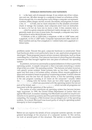
indicate the current mode: kernel (0) or user (1). !Viththeplode1:Jit!Ve2lrea]Jle
to distinguishbetween a task that is executed onbehalf of the operatingsystem
aicd one that is executeci on behalfoftheJJser, When tl~e computer systel.n1s
executing on behalf of a user application, the system is in user mode. However,
when a user application requests a service from the operating system (via a
.. system call), it must transition from user to kernel mode to fulfill the request.
/ This is shown in Figure 1.10. As we shall see, this architectural enhancement is
useful for many other aspects of system operation as well.
execute system call
Figure 1.i 0 Transition from user to kernel mode.
user mode
(mode bit =I)
kernel mode
(mode bit = 0)](https://image.slidesharecdn.com/elecnwintjql7eggtsqw-operating-system-concepts-8th-editiona4-230117160154-4fa44b38/85/Operating_System_Concepts_8th_EditionA4-pdf-35-320.jpg)
![22 Chapter 1
At system boot time, the hardware starts in kernel mode. The operating
system is then loaded and starts user applications in user mode. Whenever a
trap or interrupt occurs, the hardware switches from user mode to kernel mode
(that is, changes the state of the mode bit to 0). Thus, whenever the operating
system gains control of the computer, it is in kernel mode. The system always
switches to user mode (by setting the mode bit to 1) before passing control to
a user program.
The dual mode of operation provides us with the means for protecting the
operating system from errant users-and errant users from one another. }Ye
_(!CC011lplishthis protectionby designating someofthemachineinE;tructions~ha!
:trliJjT cal1_seJ~i:i~l11 ins trucrci}]<§l: Il1e hardware all~<'Spl·iyileg~d
instrl]ctionsto be o11ly inkern~Ll11QQ_~, If an attempt is made to
execute a privileged instruction in user mode, the hardware does not execute
the instruction but rather treats it as illegal and traps it to the operating system.
The instruction to switch to kernel mode is an example of a privileged
instruction. Some other examples include I/0 controt timer management and
interrupt management. As we shall see throughout the text, there are many
additional privileged instructions.
We can now see the life cycle of instruction execution in a computer system.
Initial control resides in the operating system, where instructions are executed
in kernel mode. When control is given to a user application, the mode is set to
user mode. Eventually, control is switched back to the operating system via an
interrupt, a trap, or a system call.
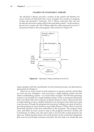
_5ysiemcalls proyide the means for auser program to ask the operating
2}'St~m to perforp:t tasks re_?erved forjhe operating syst~m gr1 the 1.lser
.12l.:Qgra1ll'sbeha,lf A system call is invoked in a variety of ways, depending
on the functionality provided by the underlying processor. In all forms, it is the
method used by a process to request action by the operating system. A system
call usually takes the form of a trap to a specific location in the interrupt vector.
This trap can be executed by a generic trap instruction, although some systems
(such as the MIPS R2000 family) have a specific syscall instruction.
When asystep1 calljs e)(ecutect it is treated by the hardware as a software
-i:rlt~rr:l.l:[if:C()iltrol passes through the interrupt vector to a service routine in
theoperating system/ and the m()de bit is set to kernel mode. The system-
caflserv1ce routine is apart of the operating system. The-kernel examines
the interrupting instruction to determine what system call has occurred; a
~ parameter indicates what type of service the user program is requesting.
Additional information needed forthe r~quest_may be passed in registers,
on the stack/ or in memory (with pointers to the memory locations passed in
registers). The kernel vedfies that the parameters are correct and legat executes
ti1erequest, and returns control to the instruction following the system call. We
describe system calls more fully in Section 2.3.
The lack of a hardware-supported dual mode can cause serious shortcom-
ings in an operating system. For instance, MS-DOS was written for the Intel
8088 architecture, which has no mode bit and therefore no dual mode. A user
program rum1ing awry can wipe out the operating system by writing over it
with data; and multiple programs are able to write to a device at the same time,
with potentially disastrous results. Recent versions of the Intel CPU do provide
dual-mode operation. Accordingly, most contemporary operating systems-
such as Microsoft Vista and Windows XP, as well as Unix, Linux, and Solaris](https://image.slidesharecdn.com/elecnwintjql7eggtsqw-operating-system-concepts-8th-editiona4-230117160154-4fa44b38/85/Operating_System_Concepts_8th_EditionA4-pdf-36-320.jpg)
![24 Chapter 1
1.7
that the concept is more general. As we shall see in Chapter 3, it is possible
to provide system calls that allow processes to create subprocesses to execute
concurrent!y.
A process needs certain resources---including CPU time, me111ory, files,
and-I;o devices:::_:_to accomplish its:task These i·esources are e!tl1er given to
the process when it is created or-allocated to it while it is running. In addition
to the various physical and logical resources that a process obtains when it is
created, various initialization data (input) may be passed along. For example,
consider a process whose function is to display the status of a file on the screen
of a terminal. The process will be given as an input the name of the file and will
execute the appropriate instructions and system calls to obtain and display
on the terminal the desired information. When the process terminates, the
operating system will reclaim any reusable resources.
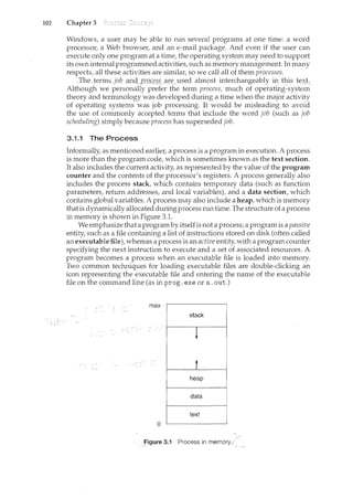
l"Ve ~_111pl:t21size that a program by itselfis nota process; a program is a
·y_assive er~!~ty, likt:tl1e C()I1terltsof a fil(?storecl_m1 c!iskL~A.ThereasC_pr(Jce~~s_1s 21~1
aCtive entity. A si-Dgl~::1hr:eaded proc~ss has on~_pr_ogra111 cou11!er s:eecifying the
nexf1il~r:Uc_tiogt()_eX~ClJte. (Threads are covered in Chapter 4.) The-execi.rtioil.
of such a process must be sequential. The CPU executes one instruction of the
process after another, until the process completes. Further, at any time, one
instruction at most is executed on behalf of the process. Thus, although two
processes may be associated with the same program, they are nevertheless
considered two separate execution sequences. A multithreaded process has
multiple program counters, each pointing to the next instruction to execute for
a given thread.
A process is the unit of work in a system. Such a system consists of a
collection of processes, some of which are operating-system processes (those
that execute system code) and the rest of which are user processes (those that
execute user code). Al]Jheseprocesses canp()t~!ltially execute concurrently-
_llY.IJ:lli}!p_l~)(_i!lg ()I'a sir1gle_C:Pl],for_~)(ample. - - - --- ----
The operating system is responsible for the following activities in connec-
tion with process management:
Scheduling processes and threads on the CPUs
Creating and deleting both user and system processes
Suspending and resuming processes
Providing mechanisms for process synchronization
Providing mechanisms for process communication
We discuss process-management techniques in Chapters 3 through 6.
As we discussed in Section 1.2.2, the main memory is central to the operation
of a modern computer system. Main memory is a large array of words or bytes,
ranging in size from hundreds of thousands to billions. Each word or byte has
its own address. Main memory is a repository of quickly accessible data shared
by the CPU and I/0 devices. The central processor reads instructions from main](https://image.slidesharecdn.com/elecnwintjql7eggtsqw-operating-system-concepts-8th-editiona4-230117160154-4fa44b38/85/Operating_System_Concepts_8th_EditionA4-pdf-38-320.jpg)
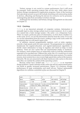
![28 Chapter 1
Main memory can be viewed as a fast cache for secondary storage, since
data in secondary storage must be copied into main memory for use, and
data must be in main memory before being moved to secondary storage for
safekeeping. The file-system data, which resides permanently on secondary
storage, may appear on several levels in the storage hierarchy. At the highest
level, the operating system may maintain a cache of file-system data in main
memory. In addition, electronic RAM disks (also known as
may be used for high-speed storage that is accessed through the file-system
interface. The bulk of secondary storage is on magnetic disks. The magnetic-
disk storage, in turn, is often backed up onto magnetic tapes or removable
disks to protect against data loss in case of a hard-disk failure. Some systems
autoinatically archive old file data from secondary storage to tertiary storage,
such as tape jukeboxes, to lower the storage cost (see Chapter 12).
The movement of information between levels of a storage hierarchy may
be either explicit or implicit, depending on the hardware design and the
controlling operating-system software. f_o].')!LStilnce,datatransfe~ from cache
_l~CPU
~'11~cl_!"~g~~!~:r-_s _is__~1sually ahardvvarefunction, with no op-erat[ii.g=sy-stern
intervention. In contrast, transfer of daTa-from- aisk to memory is usually
controlledby the-op~ra-t!:ri.g"system. -
- fn a 11ier2rrchical storage structure, the same data may appear in different
levels of the storage system. For example, suppose that an integer A that is to
be incremented by 1 is located in file B, and file B resides on magnetic disk.
The increment operation proceeds by first issuing an I/O operation to copy the
disk block on which A resides to main memory. This operation is followed by
copying A to the cache and to an internal register. Thus, the copy of A appears
in several places: on the magnetic disk, in main memory, in the cache, and in an
internal register (see Figure 1.12). Once the increment takes place in the internal
register, the value of A differs in the various storage systems. The value of A
becomes the same only after the new value of A is written from the internal
register back to the magnetic disk.
In a computing environment where only one process executes at a tim.e,
this arrangement poses no difficulties, since an access to integer A will always
be to the copy at the highest level of the hierarchy. However, in a multitasking
environment, where the CPU is switched back and -forth-among var1ous
processes~ extreme care must be taken to ensure that, if several processe~vv:is}l
i:o-accessA, then each of these processes will obtain the most recently updated
___c_=--.C. of A. - - - -
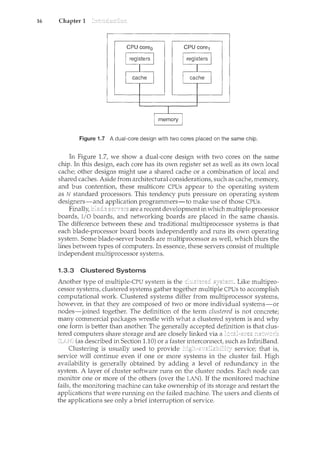
The situation becomes more complicated in a multiprocessor environment
where, in addition to maintaining internal registers, each of the CPUs also
contains a local cache (Figure 1.6). ~'"1_ su~bC1:.1l_<:_n~i£o!_l:_Il'l_~1lt,~S<2EY()f_A IJ.t~y
exist simultaneouslyinseyeral caches. Since the variousCPUs can all execute
.S:2~1c~r~~l~tly,",Ve-must1nake surethat an to the value ofA in one cache
Figure 1.12 Migration of integer A from disk to register.](https://image.slidesharecdn.com/elecnwintjql7eggtsqw-operating-system-concepts-8th-editiona4-230117160154-4fa44b38/85/Operating_System_Concepts_8th_EditionA4-pdf-42-320.jpg)
![1.10 31
increases computation speed, functionality, data availability, and reliability.
Some operating systems generalize network access as a form of file access, with
the details of networking contained in the network interface's device driver.
Others make users specifically invoke network functions. Generally, systems
contain a mix of the two modes-for example FTP and NFS. The protocols
that create a distributed system can greatly affect that system's utility and
popularity.
A in the simplest terms, is a communication path between
two or more systems. Distributed systems depend on networking for their
functionality. Networks vary by the protocols used, the distances between
nodes, and the transport media. TCP/IP is the most common network protocol,
although ATM and other protocols are in widespread use. Likewise, operating-
system support of protocols varies. Most operating systems support TCP/IP,
including the Windows and UNIX operating systems. Some systems support
proprietary protocols to suit their needs. To an operating system, a network
protocol simply needs an interface device-a network adapter, for example-
with a device driver to manage it, as well as software to handle data. These
concepts are discussed throughout this book.
Networks are characterized based on the distances between their nodes.
A computers within a room, a floor,
or a building. A N) usually links buildings, cities,
or countries. A global company may have a WAN to com1ect its offices
worldwide. These networks may run one protocol or several protocols. The
continuing advent of new technologies brings about new forms of networks.
For example, a {]'/!Al··I} could link buildings within
'.::a city. BlueTooth and 802.11 devices use wireless technology to commt.micate
over a distance of several feet, in essence creating a such
as might be found in a home.
The media to carry networks are equally varied. They include copper wires,
fiber strands, and wireless transmissions between satellites, microwave dishes,
and radios. When computing devices are connected to cellular phones, they
create a network. Even very short-range infrared communication can be used
for networking. At a rudimentary level, whenever computers communicate,
they use or create a network. These networks also vary in their performance
and reliability.
Some operating systems have taken the concept of networks and dis-
tributed systems further than the notion of providing network connectivity. A
is an operating system that provides features such
as file sharing across the network and that includes a communication scheme
that allows different processes on different computers to exchange messages.
A computer rmming a network operating system acts autonomously from all
other computers on the network, although it is aware of the network and is
able to communicate with other networked computers. A distributed operat-
ing system provides a less autonomous envirorunent: The different operating
systems comm"Lmicate closely enough to provide the illusion that only a single
operating system controls the network.
We cover computer networks and distributed systems in Chapters 16
through 18.](https://image.slidesharecdn.com/elecnwintjql7eggtsqw-operating-system-concepts-8th-editiona4-230117160154-4fa44b38/85/Operating_System_Concepts_8th_EditionA4-pdf-45-320.jpg)
![46 Chapter 1
Brookshear [2003] provides an overview of computer science in generaL
An overview of the Linux operating system is presented in Bovet and
Cesati [2006]. Solomon and Russinovich [2000] give an overview of Microsoft
Windows and considerable technical detail abmrt the systern internals and
components. Russinovich and Solomon [2005] update this information to
Windows Server 2003 and Windows XP. McDougall and Mauro [2007] cover
the internals of the Solaris operating system. Mac OS X is presented at
http: I /www. apple. com/macosx. Mac OS X internals are discussed in Singh
[2007].
Coverage of peer-to-peer systems includes Parameswaran et al. [2001],
Gong [2002], Ripeanu et al. [2002], Agre [2003], Balakrishnan et al. [2003], and
Loo [2003]. A discussion of peer-to-peer file-sharing systems can be found in
Lee [2003]. Good coverage of cluster computing is provided by Buyya [1999].
Recent advances in cluster computing are described by Ahmed [2000]. A survey
of issues relating to operating-system support for distributed systems can be
found in Tanenbaum and Van Renesse [1985].
Many general textbooks cover operating systems, including Stallings
[2000b], Nutt [2004], and Tanenbaum [2001].
Hamacher et al. [2002] describe cmnputer organization, and McDougall
and Laudon [2006] discuss multicore processors. Hennessy and Patterson
[2007] provide coverage of I/O systems and buses, and of system archi-
tecture in general. Blaauw and Brooks [1997] describe details of the archi-
tecture of many computer systems, including several from IBM. Stokes
[2007] provides an illustrated introduction to microprocessors and computer
architecture.
Cache memories, including associative memory, are described and ana-
lyzed by Smith [1982]. That paper also includes an extensive bibliography on
the subject.
Discussions concerning magnetic-disk technology are presented by Freed-
man [1983] and by Harker et al. [1981]. Optical disks are covered by Kenville
[1982], Fujitani [1984], O'Leary and Kitts [1985], Gait [1988], and Olsen and
Kenley [1989]. Discussions offloppy disks are offered by Pechura and Schoeffler
[1983] and by Sarisky [1983]. General discussions concerning mass-storage
technology are offered by Chi [1982] and by Hoagland [1985].
Kurose and Ross [2005] and Tanenbaum [2003] provide general overviews
of computer networks. Fortier [1989] presents a detailed discussion ofnetwork-
ing hardware and software. Kozierok [2005] discuss TCP in detail. Mullender
[1993] provides an overview of distributed systems. [2003] discusses
recent developments in developing embedded systems. Issues related to hand-
held devices can be found in Myers and Beigl [2003] and DiPietro and Mancini
[2003].
A full discussion of the history of open sourcing and its benefits and chal-
lenges is found in Raymond [1999]. The history of hacking is discussed in Levy
[1994]. The Free Software Foundation has published its philosophy on its Web
site: http://www.gnu.org/philosophy/free-software-for-freedom.html.
Detailed instructions on how to build the Ubuntu Linux kernel are on](https://image.slidesharecdn.com/elecnwintjql7eggtsqw-operating-system-concepts-8th-editiona4-230117160154-4fa44b38/85/Operating_System_Concepts_8th_EditionA4-pdf-60-320.jpg)

![2.5 67
Some of them are simply user interfaces to system calls; others are considerably
more complex. They can be divided into these categories:
File management. These programs create, delete, copy, rename, print,
dump, list, and generally ncanipulate files and directories.
Status information. Some programs simply ask the system for the date,
time, amount of available memory or disk space, number of users, or
similar status information. Others are more complex, providing detailed
performance, logging, and debugging information. Typically, these pro-
grams format and print the output to the terminal or other output devices
or files or display it in a window of the GUI. Some systems also support a
which is used to store and retrieve configuration information.
File modification. Several text editors may be available to create and
modify the content of files stored on disk or other storage devices. There
may also be special commands to search contents of files or perform
transformations of the text.
Programming-language support. Compilers, assemblers, debuggers, and
interpreters for common programming languages (such as C, C++, Java,
Visual Basic, and PERL) are often provided to the user with the operating
system.
Program loading and execution. Once a program is assembled or com-
piled, it must be loaded into memory to be executed. The system may
provide absolute loaders, relocatable loaders, linkage editors, and overlay
loaders. Debugging systems for either higher-level languages or machine
language are needed as well.
Communications. These programs provide the mechanism for creating
virtual comcections among processes, users, and computer systems. They
allow users to send rnessages to one another's screens, to browse Web
pages, to send electronic-mail messages, to log in remotely, or to transfer
files from one machine to another.
In addition to systems programs, most operating systems are supplied
with programs that are useful in solving common problems or performing
common operations. Such application]JJ:"Ogr!lJ1lS iitclLlde'ifT~l:l l:Jrg_wsf2r~, worg
processors an<i text f6-rinattEis,spreadsheets, database systems, compilers,
plott1i1g ana s-tafistica]-analysis packages, ancl gan1es~ - -- - - -------- -----
___ Tne viewoClne Opei;ating-sysrerri-seen b)T inost users is defined by the
application and system programs, rather than by the actual systern calls.
Consider a user's PC. When a user's computer is rumcing the Mac OS X
operating system, the user might see the GUI, featuring a mouse-and-windows
interface. Alternatively, or even in one of the windows, the user might have
a command-line UNIX shell. Both use the same set of system calls, but the
system calls look different and act in different ways. Further confusing the
user view, consider the user dual-booting from Mac OS X into Windows Vista.
Now the same user on the same hardware has two entirely different interfaces
and two sets of applications using the same physical resources. On the same](https://image.slidesharecdn.com/elecnwintjql7eggtsqw-operating-system-concepts-8th-editiona4-230117160154-4fa44b38/85/Operating_System_Concepts_8th_EditionA4-pdf-81-320.jpg)
![68 Chapter 2
2.6
hardware, then, a user can be exposed to multiple user interfaces sequentially
or concurrently.
In this section, we discuss problems we face in designing and implementing an
operating system. There are, of course, no complete solutions to such problems,
but there are approaches that have proved successful.
2.6.1 Design Goals
The first problem in designing a system is to define goals and specifications.
At the highest level, the design of the system will be affected by the choice of
hardware and the type of system: batch, time shared, single user, multiuser,
distributed, real time, or general purpose.
Beyond this highest design level, the requirements may be much harder to
specify. The requirements can, however, be divided into two basic groups: user
goals and system goals.
Users desire certain obvious properties in a system. The system should be
convenient to use, easy to learn and to use, reliable, safe, and fast. Of course,
these specifications are not particularly useful in the system design, since there
is no general agreement on how to achieve them.
A similar set of requirements can be defined by those people who must
design, create, maintain, and operate the system. The system should be easy to
design, implement, and maintain; and it should be flexible, reliable, error free,
and efficient. Again, these requirements are vague and may be interpreted in
various ways.
There is, in short, no unique solution to the problem of defining the
requirements for an operating system. The wide range of systems in existence
shows that different requirements can result in a large variety of solutions for
different environments. For example, the requirements for VxWorks, a real-
time operating system for embedded systems, must have been substantially
different from those for MVS, a large multiuser, multiaccess operating system
for IBM mainframes.
Specifying and designing an operating system is a highly creative task.
Although no textbook can tell you how to do it, general principles have
been developed in the field of software engineering, and we turn now to
a discussion of some of these principles. c -
2.6.2 Mechanisms and Policies .,
I
One important principle is the separation of policy from mechanisiil~echa::
1'lis~s (:leter111il1e hcnu !Q_c:@-son'l~tl-til1g; p()lic:les (i~termir<e .zul1dTwilCbe done.
For example, the timer construct (see Section 1.5.2) is a mechani.sril:-forensill1ng
CPU protection, but deciding how long the timer is to be set for a particular
user is a policy decision.
_]'h~_S_§122l!Cl_tig!l:()fP.Qli_cy_an_ci~T1_echanism is imp()rtant for flexibility. Policies
are likely to change across places o1:'over- time. 'rri tll'e worst case, each change
in policy would require a change in the underlying mechanism. A general
mechanism insensitive to changes in policy would be more desirable. A change](https://image.slidesharecdn.com/elecnwintjql7eggtsqw-operating-system-concepts-8th-editiona4-230117160154-4fa44b38/85/Operating_System_Concepts_8th_EditionA4-pdf-82-320.jpg)
![72 Chapter 2
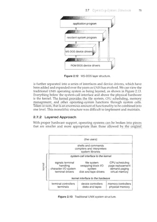
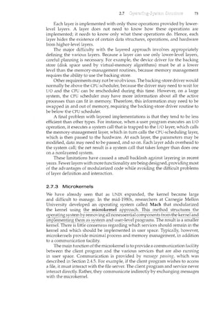
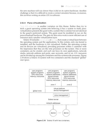
Figure 2.14 A layered operating system.
M~-:.QOi'ilncil]l'J_IX systeill~· The operating system can then retain much greater
control over the computer and over the applications that make use of that
computer. Implementers have more freedom in changing the inner workin.gs
of the system and in creating modular operating systems. Under a top-
down approach, the overall functionality and features are determined and
are separated into components. Information hiding is also important, because
it leaves programmers free to implement the low-level routines as they see fit,
provided that the external interface of the routine stays unchanged and that
the routine itself performs the advertised task.
A system can be made modular in many ways. Qne method is the layered
approach, in which the operating system is broken ii1to a 1l.umberoflayers
""(lever8J.TI1eoottom.Iiiyer.(layer 0).1stheTiarawai;e; the nig:Ytesl: (layerN)..1sfhe
user interface. This layering structure is depicted in Figure 2.14.
An operating-system layer is an implementation of an abstract object made
up of data and the operations that can manipulate those data. A typical
operating-system layer-say, layer M -consists of data structures and a set
of routines that can be invoked by higher-level layers. Layer M, in turn, can
invoke operations on lower-level layers.
The main advantage of the layered approach is simplicity of construction
and debugging. The layers are selected so that each uses functions (operations)
and services of only lower-level layers. This approach simplifies debugging
and .system verification. The first layer can be debugged without any concern
for the rest of the system, because, by definition, it uses only the basic hardware
(which is assumed correct) to implement its functions. Once the first layer is
debugged, its correct functioning can be assumed while the second layer is
debugged, and so on. If an error is found during the debugging of a particular
layer, the error must be on that layer, because the layers below it are already
debugged. Thus, the design and implementation of the system are simplified.](https://image.slidesharecdn.com/elecnwintjql7eggtsqw-operating-system-concepts-8th-editiona4-230117160154-4fa44b38/85/Operating_System_Concepts_8th_EditionA4-pdf-86-320.jpg)
![2.9 87
loops are allowed, and only specific kernel state modifications are allowed
when specifically requested. Only users with the DTrace "privileges" (or "root"
users) are allowed to use DT!·ace, as it can retrieve private kernel data (and
modify data if requested). The generated code runs in the kernel and enables
probes. It also enables consumers in user mode and enables communications
between the two.
A DT!·ace consumer is code that is interested in a probe and its results.
A consumer requests that the provider create one or more probes. When a
probe fires, it emits data that are managed by the kernel. Within the kernel,
actions called or are performed when probes
fire. One probe can cause multiple ECBs to execute if more than one consumer
is interested in that probe. Each ECB contains a predicate ("if statement") that
can filter out that ECB. Otherwise, the list of actions in the ECB is executed. The
most usual action is to capture some bit of data, such as a variable's value at
that point of the probe execution. By gathering such data, a complete picture of
a user or kernel action can be built. Further, probes firing from both user space
and the kernel can show how a user-level action caused kernel-level reactions.
Such data are invaluable for performance monitoril1.g and code optimization.
Once the probe consumer tennil1.ates, its ECBs are removed. If there are no
ECBs consuming a probe, the probe is removed. That involves rewriting the
code to remove the dtrace_probe call and put back the original code. Thus,
before a probe is created and after it is destroyed, the system is exactly the
same, as if no probing occurred.
DTrace takes care to assure that probes do not use too much memory or
CPU capacity, which could harm the running system. The buffers used to hold
the probe results are monitored for exceeding default and maximum limits.
CPU time for probe execution is monitored as well. If limits are exceeded, the
consumer is terminated, along with the offending probes. Buffers are allocated
per CPU to avoid contention and data loss.
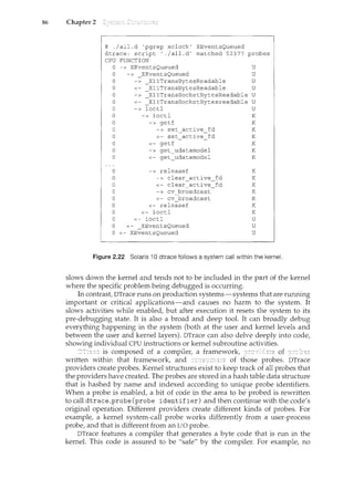
An example ofD code and its output shows some ofits utility. The following
program shows the DTrace code to enable scheduler probes and record the
amount of CPU time of each process running with user ID 101 while those
probes are enabled (that is, while the program nms):
sched:: :on-cpu
uid == 101
{
self->ts timestamp;
}
sched: : :off-cpu
self->ts
{
}
©time [execname]
self->ts = 0;
sum(timestamp- self->ts);
The output of the program, showing the processes and how much time (in
nanoseconds) they spend running on the CPUs, is shown in Figure 2.23.](https://image.slidesharecdn.com/elecnwintjql7eggtsqw-operating-system-concepts-8th-editiona4-230117160154-4fa44b38/85/Operating_System_Concepts_8th_EditionA4-pdf-101-320.jpg)
![#include <linux/errno.h>
#include <sys/syscall.h>
#include <linux/unistd.h>
_syscallO(int, helloworld);
main()
{
helloworld();
}
97
The _syscallO macro takes two arguments. The first specifies the
type of the value returned by the system call; the second is the
name of the system call. The name is used to identify the system-
call number that is stored in the hardware register before the trap
instruction is executed. If your system call requires arguments, then
a different macro (such as _syscallO, where the suffix indicates the
number of arguments) could be used to instantiate the assembly
code required for performing the system call.
Compile and execute the program with the newly built kernel.
There should be a message "hello world!" in the kernel log file
/var/log/kernel/warnings to indicate that the system call has
executed.
As a next step, consider expanding the functionality of your system call.
How would you pass an integer value or a character string to the system
call and have it printed illto the kernel log file? What are the implications
of passing pointers to data stored in the user program's address space
as opposed to simply passing an integer value from the user program to
the kernel using hardware registers?
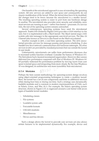
Dijkstra [1968] advocated the layered approach to operating-system desigll".
Brinch-Hansen [1970] was an early proponent of constructing an operating
system as a kernel (or nucleus) on which more complete systems can be built.
System instrumentation and dynamic tracing are described in Tamches and
Miller [1999]. DTrace is discussed in Cantrill et al. [2004]. The DTrace source
code is available at http: I I src. opensolaris. org/source/" Cheung and
Loong [1995] explore issues of operating-system structure from microkernel
to extensible systems.
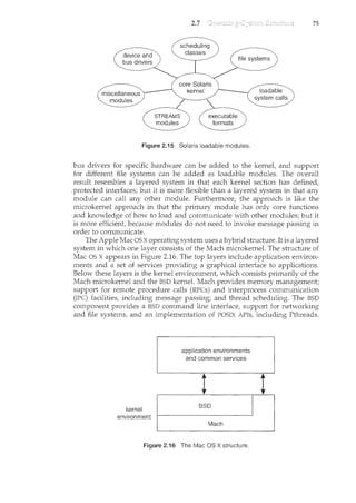
MS-DOS, Version 3.1, is described in Microsoft [1986]. Windows NT and
Windows 2000 are described by Solomon [1998] and Solomon and Russinovich
[2000]. Windows 2003 and Windows XP internals are described in Russinovich
and Solomon [2005]. Hart [2005] covers Windows system$ programming in
detail. BSD UNIX is described in McKusick et al. [1996]. Bovet and Cesati
[2006] thoroughly discuss the Linux kernel. Several UNIX systems-including
Mach-are treated in detail in Vahalia [1996]. Mac OS X is presented at](https://image.slidesharecdn.com/elecnwintjql7eggtsqw-operating-system-concepts-8th-editiona4-230117160154-4fa44b38/85/Operating_System_Concepts_8th_EditionA4-pdf-111-320.jpg)
![98 Chapter 2
http: I lwww. apple. comlmacosx and in Singh [2007]. Solaris is fully described
in McDougall and Mauro [2007].
The first operating system to provide a virtual machine was the CPI 67 on
an IBM 360167. The commercially available IBM VMI370 operating system was
derived from CP167. Details regarding Mach, a microkernel-based operating
system, canbe found in Young et al. [1987]. Kaashoeket al. [1997] present details
regarding exokernel operating systems, wherein the architecture separates
management issues from protection, thereby giving untrusted software the
ability to exercise control over hardware and software resources.
The specifications for the Java language and the Java virtual machine are
presented by Gosling et al. [1996] and by Lindholm and Yellin [1999], respec-
tively. The internal workings of the Java virtual machine are fully described
by Ven11ers [1998]. Golm et al. [2002] highlight the JX operating system; Back
et al. [2000] cover several issues in the design of Java operating systems. More
information on Java is available on the Web at http: I lwww. j avasoft. com.
Details about the implementation of VMware can be found in Sugerman et al.
[2001]. Information about the Open Virh1al Machine Format can be found at
http:llwww.vmware.comlappliancesllearnlovf.html.](https://image.slidesharecdn.com/elecnwintjql7eggtsqw-operating-system-concepts-8th-editiona4-230117160154-4fa44b38/85/Operating_System_Concepts_8th_EditionA4-pdf-112-320.jpg)

![118 Chapter 3
To illustrate the concept of cooperating processes, let's consider the
producer-consumer problem, which is a common paradigm for cooperating
processes. A producer process produces information that is consumed by a
consumer process. For example, a compiler may produce assembly code,
which is consumed by an assembler. The assembler, in turn, ncay produce
object modules, which are consumed by the loader. The producer-consumer
problem also provides a useful metaphor for the client-server paradigm. We
generally think of a server as a producer and a client as a consumer. For
example, a Web server produces (that is, provides) HTML files and images,
which are consumed (that is, read) by the client Web browser requesting the
resource.
One solution to the producer-consumer problem uses shared memory. To
allow producer and consumer processes to run concurrently, we must have
available a buffer of items that can be filled by the producer and emptied by
the consumer. This buffer will reside in a region of memory that is shared
by the producer and consumer processes. A producer can produce one item
while the consumer is consuming another item. The producer and consumer
must be synchronized, so that the consumer does not try to consume an item
that has not yet been produced.
Two types ofbuffers canbe used. The places no practical
limit on the size of the buffer. The consumer may have to wait for new items,
but the producer can always produce new items. The assumes
a fixed buffer size. In this case, the consumer must wait if the buffer is empty,
and the producer must wait if the buffer is full.
Let's look more closely at how the bounded buffer can be used to enable
processes to share memory. The following variables reside in a region of
memory shared by the producer and consumer processes:
#define BUFFER_SIZE 10
typedef struct
}item;
item buffer[BUFFER_SIZE];
int in = 0;
int out = 0;
The shared buffer is implemented as a circular array with two logical
pointers: in and out. The variable in points to the next free position in the
buffer; out points to the first full position in the buffer. The buffer is empty
when in== out; the buffer is full when ((in+ 1)% BUFFER_SIZE) == out.
The code for the producer and consumer processes is shown in Figures 3.14
and 3.15, respectively. The producer process has a local variable nextProduced
in which the new item to be produced is stored. The consumer process has a
local variable nextConsumed in which the item to be consumed is stored.
This scheme allows at most BUFFER_SIZE - 1 items in the buffer at the same
time. We leave it as an exercise for you to provide a solution where BUFFER_SIZE
items can be in the buffer at the same time. In Section 3.5.1, we illustrate the
POSIX API for shared memory.](https://image.slidesharecdn.com/elecnwintjql7eggtsqw-operating-system-concepts-8th-editiona4-230117160154-4fa44b38/85/Operating_System_Concepts_8th_EditionA4-pdf-132-320.jpg)
![3.4
item nextProduced;
while (true) {
}
I* produce an item in nextProduced *I
while ( ((in + 1) % BUFFER_SIZE) == out)
; I* do nothing *I
buffer[in] = nextProduced;
in = (in + 1) % BUFFER_SIZE;
Figure 3.'14 The producer process.
119
One issue this illustration does not address concerns the situation in which
both the producer process and the consumer process attempt to access the
shared buffer concurrently. In Chapter 6, we discuss how synchronization
among cooperating processes can be implemented effectively in a shared-
memory environment.
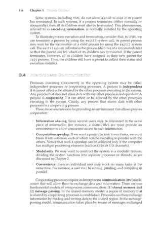
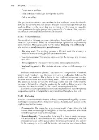
3.4.2 Message-Passing Systems
lrt Section 3.4.1, we showed how cooperating processes can communicate in a
shared-memory environment. The scheme requires that these processes share a
region of memory and that the code for accessing and manipulating the shared
memory be written explicitly by the application programmer. Another way to
achieve the same effect is for the operating system to provide the means for
cooperating processes to comm"Lmicate with each other via a message-passing
facility.
Message passing provides a mechanism to allow processes to communicate
and to synchronize their actions without sharing the same address space and
is particularly useful in a distributed environment, where the communicating
processes may reside on different computers connected by a network. For
example, a chat program used on the World Wide Web could be designed so
that chat participants communicate with one another by exchanging messages.
A message-passing facility provides at least two operations: send(message)
and receive(message). Messages sent by a process can be of either fixed
or variable size. If only fixed-sized messages can be sent, the system-level
implementation is straightforward. This restriction, however, makes the task
item nextConsumed;
while (true) {
}
while (in == out)
; II do nothing
nextConsumed = buffer[out];
out = (out + 1) % BUFFER_SIZE;
I* consume the item in nextConsumed *I
Figure 3.15 The consumer process.](https://image.slidesharecdn.com/elecnwintjql7eggtsqw-operating-system-concepts-8th-editiona4-230117160154-4fa44b38/85/Operating_System_Concepts_8th_EditionA4-pdf-133-320.jpg)
![130 Chapter 3
import java.net.*;
import java.io.*;
public class DateServer
{
}
public static void main(String[] args) {
try {
}
}
ServerSocket sock= new ServerSocket(6013);
II now listen for connections
while (true) {
}
Socket client= sock.accept();
PrintWriter pout = new
PrintWriter(client.getOutputStream(), true);
II write the Date to the socket
pout.println(new java.util.Date().toString());
II close the socket and resume
II listening for connections
client. close() ;
catch (IOException ioe) {
System.err.println(ioe);
}
Figure 3.19 Date server.
Java program shown in Figure 3.20. The client creates a Socket and requests
a connection with the server at IP address 127.0.0.1 on port 6013. Once the
connection is madef the client can read from the socket using normal stream
I/0 statements. After it has received the date from the serverf the client closes
the socket and exits. The IP address 127.0.0.1 is a special IP address known as the
When a computer refers to IP address 127.0.0.t it is referring to itself.
This mechanism allows a client and server on the same host to communicate
using the TCP/IP protocol. The IP address 127.0.0.1 could be replaced with the
IP address of another host running the date server. In addition to an IP addressf
an actual host namef such as www.westminstercollege.eduf can be used as well.
Communication using sockets-although common and efficient-is con-
sidered a low-level form of communication between distributed processes.
One reason is that sockets allow only an unstructured stream of bytes to be
exchanged between the communicating threads. It is the responsibility of the
client or server application to impose a structure on the data. In the next two
subsectionsf we look at two higher-level methods of communication: remote
procedure calls (RPCs) and pipes.](https://image.slidesharecdn.com/elecnwintjql7eggtsqw-operating-system-concepts-8th-editiona4-230117160154-4fa44b38/85/Operating_System_Concepts_8th_EditionA4-pdf-144-320.jpg)
![3.6
import java.net.*;
import java.io.*;
public class DateClient
{
}
public static void main(String[] args) {
try {
}
}
//make connection to server socket
Socket sock= new Socket("127.0.0.1",6013);
InputStream in= sock.getinputStream();
BufferedReader bin = new
BufferedReader(new InputStreamReader(in));
II read the date from the socket
String line;
while ( (line = bin.readLine()) !=null)
System.out.println(line);
II close the socket connection
sock. close() ;
catch (IDException ioe) {
System.err.println(ioe);
}
Figure 3.20 Date client.
3.6.2 Remote Procedure Calls
131
One of the most common forms of remote service is the RPC paradigm, which
we discussed briefly in Section 3.5.2. The RPC was designed as a way to
abstract the procedure-call mechanism for use between systems with network
connections. It is similar in many respects to the IPC mechanism described in
Section 3.4, and it is usually built on top of such a system. Here, howeve1~
because we are dealing with an environment in which the processes are
executing on separate systems, we must use a message-based communication
scheme to provide remote service. In contrast to the IPC facility, the messages
exchanged in RPC communication are well structured and are thus no longer
just packets of data. Each message is addressed to an RPC daemon listening to
a port on the remote system, and each contains an identifier of the ftmction
to execute and the parameters to pass to that function. The function is then
executed as requested, and any output is sentback to the requester in a separate
message.
A port is simply a number included at the start of a message packet. Whereas
a system normally has one network address, it can have many ports within
that address to differentiate the many network services it supports. If a rencote
process needs a service, it addresses a message to the proper port. For instance,](https://image.slidesharecdn.com/elecnwintjql7eggtsqw-operating-system-concepts-8th-editiona4-230117160154-4fa44b38/85/Operating_System_Concepts_8th_EditionA4-pdf-145-320.jpg)
![134 Chapter 3
The RPC scheme is useful in implementing a distribLited file system
(Chapter 17). Such a system can be implemented as a set of RPC daemons
and clients. The messages are addressed to the distributed file system port on a
server on which a file operation is to take place. The message contains the disk
operation to be performed. The disk operation might be read, write, rename,
delete, or status, corresponding to the usual file-related system calls. The
return message contains any data resulting from that call, which is executed by
the DFS daemon on behalf of the client. For instance, a message might contain
a request to transfer a whole file to a client or be limited to a simple block
request. In the latter case, several such requests may be needed if a whole file
is to be transferred.
3.6.3 Pipes
A acts as a conduit allowin.g two processes to communicate. Pipes were
one of the first IPC mechanisms in early UNIX systems and typically provide one
of the simpler ways for processes to communicate with one another, although
they also have some limitations. In implementing a pipe, four issues must be
considered:
Does the pipe allow unidirectional communication or bidirectional com-
munication?
If two-way communication is allowed, is it half duplex (data can travel
only one way at a time) or full duplex (data can travel in both directions
at the same time)?
Must a relationship (such as parent-child) exist between the commLmicat-
ing processes?
Can the pipes communicate over a network, or must the communicating
processes reside on the same machine?
In the following sections, we explore two common types of pipes used on both
UNIX and Windows systems.
3.6.3.1 Ordinary Pipes
Ordinary pipes allow two processes to communicate in standard producer-
consumer fashion; the producer writes to one end of the (the
and the consumer reads from the other end (the a result, ordinary
pipes are unidirectional, allowing only one-way communication. If two-way
communication is required, two pipes must be used, with each pipe sending
data in a different direction. We next illustrate constructing ordinary pipes
on both UNIX and Windows systems. In both program examples, one process
writes the message Greetings to the pipe, while the other process reads this
message front the pipe.
On UNIX systems, ordinary pipes are constructed using the function
pipe (int fd [])
This function creates a pipe that is accessed through the int fd [] file
descriptors: fd [0] is the read-end of the pipe, and fd [1] is the write end.](https://image.slidesharecdn.com/elecnwintjql7eggtsqw-operating-system-concepts-8th-editiona4-230117160154-4fa44b38/85/Operating_System_Concepts_8th_EditionA4-pdf-148-320.jpg)
![3.6 135
parent child
fd(O) fd(1) fd(O) fd(1)
U-(- p i p - e-oU
Figure 3.22 File descriptors for an ordinary pipe.
UNIX treats a pipe as a special type of file; thus, pipes can be accessed using
ordinary read() and write() system calls.
An ordinary pipe cannot be accessed from outside the process that creates
it. Thus, typically a parent process creates a pipe and uses it to comnmnicate
with a child process it creates via fork(). Recall from Section 3.3.1 that a child
process inherits open files from its parent. Since a pipe is a special type of file,
the child inherits the pipe from its parent process. Figure 3.22 illustrates the
relationship of the file descriptor fd to the parent and child processes.
In the UNIX progranc shown in Figure 3.23, the parent process creates a
pipe and then sends a fork() call creating the child process. What occurs after
the fork() call depends on how the data are to flow through the pipe. In this
instance, the parent writes to the pipe and the child reads from it. It is important
to notice that both the parent process and the child process initially close their
unused ends of the pipe. Although the program shown in Figure 3.23 does not
require this action, it is an important step to ensure that a process reading from
the pipe can detect end-of-file (read() returns 0) when the writer has closed
its end of the pipe.
#include <sys/types.h>
#include <stdio.h>
#include <string.h>
#include <unistd.h>
#define BUFFER_SIZE 25
#define READ_END 0
#define WRITE_END 1
int main(void)
{
char write_msg[BUFFER_SIZE]
char read_msg[BUFFER_SIZE];
int fd[2];
pid_t pid;
"Greetings";
program continues in Figure 3.24
Figure 3.23 Ordinary pipes in UNIX.](https://image.slidesharecdn.com/elecnwintjql7eggtsqw-operating-system-concepts-8th-editiona4-230117160154-4fa44b38/85/Operating_System_Concepts_8th_EditionA4-pdf-149-320.jpg)
![136 Chapter 3
}
I* create the pipe *I
if (pipe(fd) == -1) {
fprintf(stderr,"Pipe failed");
return 1;
}
I* fork a child process *I
pid = fork();
if (pid < 0) { I* error occurred *I
fprintf(stderr, "Fork Failed");
return 1;
}
if (pid > 0) { I* parent process *I
}
I* close the unused end of the pipe *I
close(fd[READ_END]);
I* write to the pipe *I
write(fd[WRITE_END], write_msg, strlen(write_msg)+1);
I* close the write end of the pipe *I
close(fd[WRITE_END]);
else { I* child process *I
}
I* close the unused end of the pipe *I
close(fd[WRITE_END]);
I* read from the pipe *I
read(fd[READ_END], read_msg, BUFFER_SIZE);
printf ("read %s", read_msg) ;
I* close the write end of the pipe *I
close(fd[READ_END]);
return 0;
Figure 3.24 Continuation of Figure 3.23 program.
Ordinary pipes on Windows systems are termed and
they behave similarly to their UNIX counterparts: they are unidirectional and
employ parent-child relationships between the communicating processes.
In addition, reading and writing to the pipe can be accomplished with the
ordinary ReadFile () and WriteFile () functions. The Win32 API for creating
pipes is the CreatePipe () function, which is passed four parameters: separate
handles for (1) reading and (2) writing to the pipe, as well as (3) an instance of
the STARTUPINFO structure, which is used to specify that the child process is to](https://image.slidesharecdn.com/elecnwintjql7eggtsqw-operating-system-concepts-8th-editiona4-230117160154-4fa44b38/85/Operating_System_Concepts_8th_EditionA4-pdf-150-320.jpg)
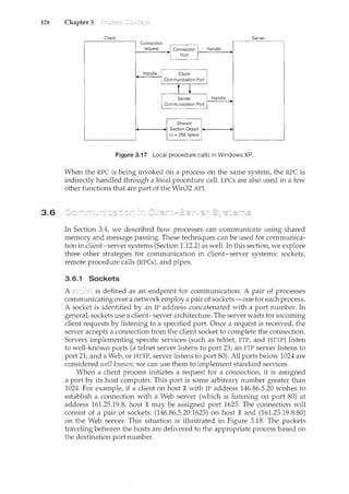
![3.6
#include <stdio.h>
#include <stdlib.h>
#include <windows.h>
#define BUFFER_SIZE 25
int main(VOID)
{
HANDLE ReadHandle, WriteHandle;
STARTUPINFO si;
PROCESS_INFORMATION pi;
char message [BUFFER_SIZE] "Greetings";
DWORD written;
program continues in Figure 3.26
Figure 3.25 Windows anonymous pipes- parent process.
137
inherit the handles of the pipe. Furthermore, (4) the size of the pipe (in bytes)
may be specified.
Figure 3.25 illustrates a parent process creating an anonymous pipe for
communicating with its child. Unlike UNIX systems, in which a child process
automatically inherits a pipe created by its parent, Windows requires the
programmer to specify which attributes the child process will inherit. This is
accomplished by first initializing the SECURITY--ATTRIBUTES structure to allow
handles to be inherited and then redirecting the child process's handles for
standard input or standard output to the read or write handle of the pipe.
Since the child will be reading from the pipe, the parent must redirect the
child's standard input to the read handle of the pipe. Furthermore, as the pipes
are half duplex, it is necessary to prohibit the child from inheriting the write
end of the pipe. Creating the child process is similar to the program in Figure
3.12, except that the fifth parameter is set to TRUE, indicating that the child
process is to inherit designated handles from its parent. Before writing to the
pipe, the parent first closes its unused read end of the pipe. The child process
that reads from the pipe is shown in Figure 3.27. Before reading from the pipe,
this program obtains the read handle to the pipe by invoking GetStdHandle ().
Note that ordinary pipes require a parent-child relationship between the
communicating processes on both UNIX and Windows systems. This means
that these pipes can be used only for communication between processes on the
same machine.
3.6.3.2 Named Pipes
Ordinary pipes provide a simple communication mechanism between a pair
of processes. However, ordinary pipes exist only while the processes are
communicating with one another. On both UNIX and Windows systems, once
the processes have finished communicating and terminated, the ordinary pipe
ceases to exist.](https://image.slidesharecdn.com/elecnwintjql7eggtsqw-operating-system-concepts-8th-editiona4-230117160154-4fa44b38/85/Operating_System_Concepts_8th_EditionA4-pdf-151-320.jpg)
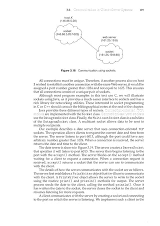
![3.6
#include <stdio.h>
#include <windows.h>
#define BUFFER_STZE 25
int main(VOID)
{
HANDLE Readhandle;
CHAR buffer [BUFFER_SIZE] ;
DWORD read;
I* get the read handle of the pipe *I
ReadHandle GetStdHandle (STD_INPULI-IANDLE) ;
I* the child reads from the pipe *I
139
if (ReadFile (ReadHandle, buffer, BUFFER_SIZE, &read, NULL))
printf("child read %s",buffer);
else
fprintf(stderr, "Error reading from pipe");
return 0;
}
Figure 3.27 Windows anonymous pipes -child process.
communication. In fact, in a typical scenario, a named pipe has several
writers. Additionally, named pipes continue to exist after communicating
processes have finished. Both UNIX and Windows systems support named
pipes, although the details of implementation vary greatly. Next, we explore
named pipes in each of these systems.
Named pipes are referred to as FIFOs in UNIX systems. Once created, they
appear as typical files in the file system. A FIFO is created with the mkfifo ()
system call and manipulated with the ordinary open(), read(), write(),
and close () system calls. It will contirme to exist m<til it is explicitly deleted
from the file system. Although FIFOs allow bidirectional communication, only
half-duplex transmission is permitted. If data must travel in both directions,
two FIFOs are typically used. Additionally, the communicating processes must
reside on the same machine; sockets (Section 3.6.1) mustbe used ifintermachine
communication is required.
Named pipes on Windows systems provide a richer communication mech-
anism than their UNIX counterparts. Full-duplex communication is allowed,
and the communicating processes may reside on either the same or different
machines. Additionally, only byte-oriented data may be transmitted across a
UNIX FTFO, whereas Windows systems allow either byte- or message-oriented
data. Named pipes are created with the CreateNamedPipe () function, and a
client can connect to a named pipe using ConnectNamedPipe (). Communi-
cation over the named pipe can be accomplished using the ReadFile () and
WriteFile () functions.](https://image.slidesharecdn.com/elecnwintjql7eggtsqw-operating-system-concepts-8th-editiona4-230117160154-4fa44b38/85/Operating_System_Concepts_8th_EditionA4-pdf-153-320.jpg)
![145
Write an echo server using the Java networking API described in
Section 3.6.1. This server will wait for a client connection using the
accept () method. When a client connection is received, the server will
loop, perfonning the following steps:
Read data from the socket into a buffer.
Write the contents of the buffer back to the client.
The server will break out of the loop only when it has determined that
the client has closed the connection.
The server shown in Figure 3.19 uses the java. io. BufferedReader
class. BufferedReader extends the java. io. Reader class, which is
used for reading character streams. However, the echo server cannot
guarantee that it will read characters from clients; it may receive binary
data as well. The class java. io. InputStream deals with data at the byte
level rather than the character level. Thus, this echo server must use an
object that extends java. io. InputStrearn. The read() method in the
java. io. InputStrearn class returns -1 when the client has closed its
end of the socket connection.
3.17 In Exercise 3.13, the child process must output the Fibonacci sequence,
since the parent and child have their own copies of the data. Another
approach to designing this program is to establish a shared-memory
segment between the parent and child processes. This technique allows
the child to write the contents of the Fibonacci sequence to the shared-
memory segment and has the parent output the sequence when the child
completes. Because the memory is shared, any changes the child makes
will be reflected in the parent process as well.
This program will be structured using POSIX shared memory
as described in Section 3.5.1. The program first requires creating the
data structure for the shared-memory segment. This is most easily
accomplished using a struct. This data structure will contain two items:
(1) a fixed-sized array of size MALSEQUENCE that will hold the Fibonacci
values and (2) the size of the sequence the child process is to generate-
sequence_size, where sequence_size :::: MALSEQUENCE. These items
can be represented in a struct as follows:
#define MAX_SEQUENCE 10
typedef struct {
long fib_sequence[MAX_SEQUENCE];
int sequence_size;
} shared_data;
The parent process will progress thmugh the following steps:
a. Accept the parameter passed on the command line and perform
error checking to ensure that the parameter is :::: MAX_SEQUENCE.
b. Create a shared-memory segment of size shared_data.
c. Attach the shared-memory segment to its address space.](https://image.slidesharecdn.com/elecnwintjql7eggtsqw-operating-system-concepts-8th-editiona4-230117160154-4fa44b38/85/Operating_System_Concepts_8th_EditionA4-pdf-159-320.jpg)
![152 Chapter 3
ipcs command to list all message queues and the ipcrm command to
remove existing message queues. The ipcs command lists the msqid of
all message queues on the system. Use ipcrm to remove message queues
according to their msqid. For example, if msqid 163845 appears with the
output of ipcs, it can be deleted with the following command:
ipcrm -q 163845
Interprocess communication in the RC 4000 system is discussed by Brinch-
Hansen [1970]. Schlichting and Schneider [1982] discuss asynchronous
message-passing prirnitives. The IPC facility implemented at the user level is
described by Bershad et al. [1990].
Details of interprocess communication in UNIX systems are presented by
Gray [1997]. Barrera [1991] and Vahalia [1996] describe interprocess commu-
nication in the Mach system. Russinovich and Solomon [2005], Solomon and
Russinovich [2000], and Stevens [1999] outline interprocess communication
in Windows 2003, Windows 2000 and UNIX respectively. Hart [2005] covers
Windows systems programming in detail.
The implementation of RPCs is discussed by Birrell and Nelson [1984].
Shrivastava and Panzieri [1982] describes the design of a reliable RPC mecha-
nism, and Tay and Ananda [1990] presents a survey of RPCs. Stankovic [1982]
and Stmmstrup [1982] discuss procedure calls versus message-passing com-
munication. Harold [2005] provides coverage of socket programming in Java.
Hart [2005] and Robbins and Robbins [2003] cover pipes in Windows and UNIX
systems, respectively.](https://image.slidesharecdn.com/elecnwintjql7eggtsqw-operating-system-concepts-8th-editiona4-230117160154-4fa44b38/85/Operating_System_Concepts_8th_EditionA4-pdf-166-320.jpg)
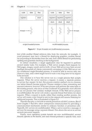
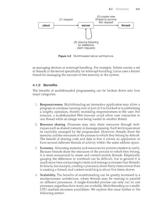
![156 Chapter 4
time
Figure 4.3 Concurrent execution on a single-core system.
4.1.3 Multicore Programming
A recent trend in system design has been to place multiple computing cores on
a single chip, where each core appears as a separate processor to the operating
system (Section 1.3.2). Multithreaded programming provides a mechanism
for more efficient use of multiple cores and improved concurrency. Consider
an application with four threads. On a system with a single computing core,
concurrency merely means that the execution of the threads will be interleaved
over time (Figure 4.3), as the processing core is capable of executing only one
thread at a time. On a system with multiple cores, however, concurrency means
that the threads can run in parallel, as the system can assign a separate thread
to each core (Figure 4.4).
The trend towards multicore systems has placed pressure on system
designers as well as application programmers to make better use ofthe multiple
computing cores. Designers of operating systems must write scheduling
algorithms that use multiple processing cores to allow the parallel execution
shown in Figure 4.4. For application programmers, the challenge is to modify
existing programs as well as design new programs that are multithreaded to
take advantage of multicore systems. In general, five areas present challenges
in programming for multicore systems:
Dividing activities. This involves examining applications to find areas
that can be divided into separate, concurrent tasks and thus can run in
parallel on individual cores.
Balance. While identifying tasks that can run in parallel, programmers
must also ensure that the tasks perform equal work of equal value. In
some instances, a certain task may not contribute as much value to the
overall process as other tasks; using a separate execution core to run that
task may not be worth the cost.
Data splitting. Just as applications are divided into separate tasks, the
data accessed and manipulated by the tasks must be divided to run on
separate cores.
core 1
l<T1 I T3 T1 T3
I Ti
core 2
[i] T4 T2 T4
I
Tz
time
Figure 4.4 Parallel execution on a multicore system.](https://image.slidesharecdn.com/elecnwintjql7eggtsqw-operating-system-concepts-8th-editiona4-230117160154-4fa44b38/85/Operating_System_Concepts_8th_EditionA4-pdf-170-320.jpg)
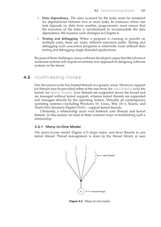
![160 Chapter 4
the Java thread API is generally implemented using a thread library available
on the host system. This means that on Windows systems, Java threads are
typically implemented using the Win32 API; UNIX and Linux systems often use
Pthreads.
In the remainder of this section, we describe basic thread creation using
these three thread libraries. As an illustrative example, we design a multi-
threaded program that performs the summation of a non-negative integer in a
separate thread using the well-known summation function:
N
sum= I~>
i=O
For example, if N were 5, this function would represent the summation of
integers from 0 to 5, which is 15. Each of the three programs will be n.m with
the upper bounds of the summation entered on the command line; thus, if the
user enters 8, the summation of the integer values from 0 to 8 will be output.
4.3.1 Pthreads
refers to the POSIX standard (IEEE 1003.lc) defining an API for thread
creation and synchronization. This is a specification for thread behavim~ not an
implementation. Operating system designers may implement the specification in
any way they wish. Numerous systems implement the Pthreads specification,
including Solaris, Linux, Mac OS X, and Tru64 UNIX. Shareware implementations
are available in the public domain for the various Windows operating systems
as well.
The C program shown in Figure 4.9 demonstrates the basic Pthreads API for
constructing a multithreaded program that calculates the summation of a non-
negative integer in a separate thread. In a Pthreads program, separate threads
begin execution in a specified function. In Figure 4.9, this is the runner()
function. When this program begins, a single thread of control begins in
main (). After some initialization, main () creates a second thread that begins
control in the runner () function. Both threads share the global data sum.
Let's look more closely at this program. All Pthreads programs must
include the pthread. h header file. The statement pthread_t tid declares
the identifier for the thread we will create. Each thread has a set of attributes,
including stack size and scheduling information. The pthread_attr_t attr
declaration represents the attributes for the thread. We set the attributes in the
function call pthread_attr_init (&attr). Because we did not explicitly set
any attributes, we use the default attributes provided. (In Chapter 5, we discuss
some of the scheduling attributes provided by the Pthreads API.) A separate
thread is created with the pthread_create () function call. In addition to
passirtg the thread identifier and the attributes for the thread, we also pass the
name of the function where the new thread will begin execution-in this case,
the runner () function. Last, we pass the integer parameter that was provided
on the command line, argv [1].
At this point, the program has two threads: the initial (or parent) thread
in main() and the summation (or child) thread performing the summation](https://image.slidesharecdn.com/elecnwintjql7eggtsqw-operating-system-concepts-8th-editiona4-230117160154-4fa44b38/85/Operating_System_Concepts_8th_EditionA4-pdf-174-320.jpg)
![4.3
#include <pthread.h>
#include <stdio.h>
int sum; I* this data is shared by the thread(s) *I
void *runner(void *param); I* the thread *I
int main(int argc, char *argv[])
{
}
pthread_t tid; I* the thread identifier *I
pthread_attr_t attr; I* set of thread attributes *I
if (argc != 2) {
}
fprintf(stderr,"usage: a.out <integer value>n");
return -1;
if (atoi(argv[1]) < 0) {
}
fprintf(stderr,"%d must be>= 0n",atoi(argv[1]));
return -1;
I* get the default attributes *I
pthread_attr_init(&attr);
I* create the thread *I
pthread_create(&tid,&attr,runner,argv[1]);
I* wait for the thread to exit *I
pthread_join(tid,NULL);
printf("sum = %dn",sum);
I* The thread will begin control in this function *I
void *runner(void *param)
{
}
inti, upper= atoi(param);
sum = 0;
for (i = 1; i <= upper; i++)
sum += i;
pthread_exit (0) ;
Figure 4.9 Multithreaded C program using the Pthreads API.
161
operation in the runner() function. After creating the summation threadf
the parent thread will wait for it to complete by calling the pthread_j oin ()
function. The summation thread will complete when it calls the function
pthread_exit (). Once the summation thread has returnedf the parent thread
will output the value of the shared data sum.](https://image.slidesharecdn.com/elecnwintjql7eggtsqw-operating-system-concepts-8th-editiona4-230117160154-4fa44b38/85/Operating_System_Concepts_8th_EditionA4-pdf-175-320.jpg)
![4.3
#include <Windows.h>
#include <stdio.h>
DWORD Sum; I* data is shared by the thread(s) *I
I* the thread runs in this separate function *I
DWORD WINAPI Sumrnation(LPVOID Param)
{
}
DWORD Upper = *(DWORD*)Param;
for (DWORD i = 0; i <= Upper; i++)
Sum += i;
return 0;
int main(int argc, char *argv[])
{
}
DWORD Threadid;
HANDLE ThreadHandle;
int Param;
I* perform some basic error checking *I
if (argc != 2) {
}
fprintf(stderr,"An integer parameter is requiredn");
return -1;
Param = atoi(argv[1]);
if (Param < 0) {
}
fprintf(stderr,"An integer>= 0 is requiredn");
return -1;
II create the thread
ThreadHandle = CreateThread(
NULL, II default security attributes
0, II default stack size
Summation, II thread function
&Param, II parameter to thread function
0, II default creation flags
&Threadid); II returns the thread identifier
if (ThreadHandle != NULL) {
}
II now wait for the thread to finish
WaitForSingleObject(ThreadHandle,INFINITE);
II close the thread handle
CloseHandle(ThreadHandle);
printf("surn = %dn" ,Sum);
Figure 4.10 Multithreaded C program using the Win32 API.
163](https://image.slidesharecdn.com/elecnwintjql7eggtsqw-operating-system-concepts-8th-editiona4-230117160154-4fa44b38/85/Operating_System_Concepts_8th_EditionA4-pdf-177-320.jpg)
![164 Chapter 4
class Sum
{
}
private int sum;
public int getSum() {
return sum;
}
public void setSum(int sum) {
this.sum sum;
}
class Summation implements Runnable
{
}
private int upper;
private Sum sumValue;
public Summation(int upper, Sum sumValue) {
this.upper = upper;
this.sumValue = sumValue;
}
public void run() {
int sum = 0;
}
for (int i = 0; i <= upper; i++)
sum += i;
sumValue.setSum(sum);
public class Driver
{
}
public static void main(String[] args) {
if (args.length > 0) {
}
if (Integer.parseint(args[O]) < 0)
System.err.println(args[O] + "must be>= 0.");
else {
II create the object to be shared
Sum sumObject = new Sum();
int upper= Integer.parseint(args[O]);
Thread thrd =new Thread(new Summation(upper, sumObject));
thrd.start();
try {
thrd. join () ;
System.out.println
("The sum of "+upper+" is "+sumObject.getSum());
} catch (InterruptedException ie) { }
}
else
System.err.println("Usage: Summation <integer value>"); }
Figure 4.11 Java program for the summation of a non-negative integer.](https://image.slidesharecdn.com/elecnwintjql7eggtsqw-operating-system-concepts-8th-editiona4-230117160154-4fa44b38/85/Operating_System_Concepts_8th_EditionA4-pdf-178-320.jpg)
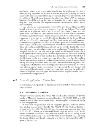
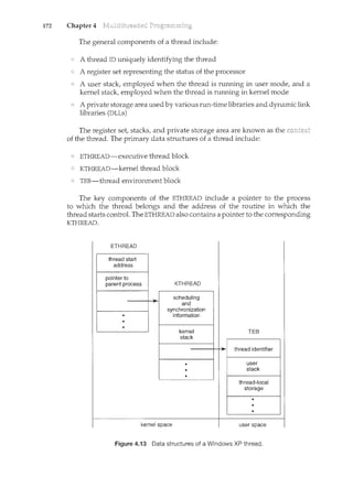
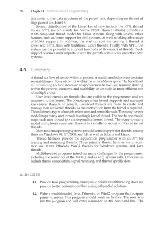
![175
program will then create a separate thread that outputs all the prime
numbers less than or equal to the number entered by the user.
4.3 Which of the following components of program state are shared across
threads in a multithreaded process?
a. Register values
b. Heap memory
c. Global variables
d. Stack memory
4.4 The program shown in Figure 4.14 uses the Pthreads API. What would
be the output from the program at LINE c and LINE P?
#include <pthread.h>
#include <stdio.h>
int value = 0;
void *runner(void *param); I* the thread *I
int main(int argc, char *argv[])
{
int pid;
pthread_t tid;
pthread_attr_t attr;
}
pid = fork();
if (pid == 0) { I* child process *I
pthread_attr_init(&attr);
pthread_create(&tid,&attr,runner,NULL);
pthread_join(tid,NULL);
printf("CHILD: value= %d",value); I* LINE C *I
}
else if (pid > 0) { I* parent process *I
wait(NULL);
printf("PARENT: value= %d",value); I* LINE P *I
}
void *runner(void *param) {
value = 5;
pthread_exit (0);
}
Figure 4.14 C program for Exercise 4.4.](https://image.slidesharecdn.com/elecnwintjql7eggtsqw-operating-system-concepts-8th-editiona4-230117160154-4fa44b38/85/Operating_System_Concepts_8th_EditionA4-pdf-189-320.jpg)
![178 Chapter 4
The Server
The server will listen to port 6052 waiting for client connections. When
a client connection is made, the server will service the connection in a separate
thread and will resume listening for additional client connections. Once a
client makes a connection to the server, the client will write the IP name it
wishes the server to resolve-such as www. westminstercollege. edu-
to the socket. The server thread will read this IP name from the socket and
either resolve its IP address or, if it cannot locate the host address, catch an
UnknownHostException. The server will write the IP address back to the
client or, in the case of an UnknownHostException, will write the message
"Unable to resolve host <host name>." Once the server has written
to the client, it will close its socket connection.
The Client
Initially, write just the server application and connect to it via telnet.
For example, assuming the server is running on the localhost a telnet session
would appear as follows. (Client responses appear in
telnec localhost 6052
Connected to localhost.
Escape character is 'A]'.
i~/VVH "'destrninstercollege. edu
146.86.1.17
Connection closed by foreign host.
By initiallyhaving telnet act as a client, you can more easily debug any problems
you may have with your server. Once you are convinced your server is working
properly, you can write a client application. The client will be passed the IP
name that is to be resolved as a parameter. The client will open a socket
connection to the server and then write the IF name that is to be resolved. It
will then read the response sent back by the server. As an example, if the client
is named NSClient, it is invoked as follows:
java NSClient www.westminstercollege.edu
and the server will respond with the corresponding IF address or "unknown
host" message. Once the client has output the IF address, it will close its socket
connection.
Project 2: Matrix Multiplication Project
Given two matrices, A and B, where matrix A contains M rows and K columns
and matrix B contains K rows and N columns, the of A and B
is matrix C, where C contains M rows and N coh.11m1s. The entry in matrix C
for row i, column j (C.j) is the sum of the products of the elements for row i
in matrix A and column j in matrix B. That is,](https://image.slidesharecdn.com/elecnwintjql7eggtsqw-operating-system-concepts-8th-editiona4-230117160154-4fa44b38/85/Operating_System_Concepts_8th_EditionA4-pdf-192-320.jpg)
![179
K
C,j = L A;,11 X Bn,j
11=:1
For example, if A is a 3-by-2 matrix and B is a 2-by-3 m.atrix, element C3,1 is
the sum of A3,1 x B1.1 and A3,2 x B2,1·
For this project, calculate each element C;,j in a separate worker thread. This
will involve creating M x N worker threads. The main-or parent-thread
will initialize the matrices A and B and allocate sufficient memory for matrix
C, which will hold the product of matrices A and B. These matrices will be
declared as global data so that each worker thread has access to A, B, and C.
Matrices A and B can be initialized statically, as shown below:
#define M3
#define K 2
#define N 3
int A [M] [K]
int B [K] [N]
int C [M] [N] ;
{ {1,4}, {2,5}, {3,6} };
{ {8,7,6}, {5,4,3} };
Alternatively, they can be populated by reading in values from a file.
Passing Parameters to Each Thread
The parent thread will create M x N worker threads, passing each worker the
values of row i and column j that it is to use in calculating the matrix product.
This requires passing two parameters to each thread. The easiest approach with
Pthreads and Win32 is to create a data structure using a struct. The members
of this structure are i and j, and the structure appears as follows:
I* structure for passing data to threads *I
struct v
{
};
int i; I* row *I
int j; I* column *I
Both the Pthreads and Win32 programs will create the worker threads
using a strategy similar to that shown below:
I* We have to create M * N worker threads *I
for (i = 0; i < M, i++)
}
for (j = 0; j < N; j++ ) {
}
struct v *data= (struct v *) rnalloc(sizeof(struct v));
data->i = i;
data->j = j;
I* Now create the thread passing it data as a parameter *I](https://image.slidesharecdn.com/elecnwintjql7eggtsqw-operating-system-concepts-8th-editiona4-230117160154-4fa44b38/85/Operating_System_Concepts_8th_EditionA4-pdf-193-320.jpg)
![180 Chapter 4
public class WorkerThread implements Runnable
{
}
private int row;
private int col;
private int [] [] A;
private int [] [] B;
private int[] [] C;
public WorkerThread(int row, int col, int[] [] A,
}
int [] [] B, int [] [] C) {
this.row =row;
this.col = col;
this.A A;
this.B
this.C
B·
'
C;
public void run() {
I* calculate the matrix product in C[row] [col] *I
}
Figure 4.15 Worker thread in Java.
The data pointer will be passed to either the pthread_create () (Pthreads)
function or the CreateThread () (Win32) function, which in turn will pass it
as a parameter to the function that is to run as a separate thread.
Sharing of data between Java threads is different from sharing between
threads in Pthreads or Win32. One approach is for the main thread to create
and initialize the matrices A, B, and C. This main thread will then create the
worker threads, passing the three matrices-along with row i and column j-
to the constructor for each worker. Thus, the outline of a worker thread appears
in Figure 4.15.
Waiting for Threads to Complete
Once all worker threads have completed, the main thread will output the
product contained in matrix C. This requires the main thread to wait for
all worker threads to finish before it can output the value of the matrix
product. Several different strategies can be used to enable a thread to wait
for other threads to finish. Section 4.3 describes how to wait for a child
thread to complete using the Win32, Pthreads, and Java thread libraries.
Win32 provides the WaitForSingleObj ect () function, whereas Pthreads
and Java use pthread_j oin () and join(), respectively. However, in these
programming examples, the parent thread waits for a single child thread to
finish; completing this exercise will require waiting for multiple threads.
In Section 4.3.2, we describe the WaitForSingleObj ect () function, which
is used to wait for a single thread to finish. However, the Win32 API also
provides the WaitForMultipleDbj ects () function, which is used when
waiting for multiple threads to complete. WaitForMultipleObjectsO is
passed four parameters:](https://image.slidesharecdn.com/elecnwintjql7eggtsqw-operating-system-concepts-8th-editiona4-230117160154-4fa44b38/85/Operating_System_Concepts_8th_EditionA4-pdf-194-320.jpg)
![#define NUM_THREADS 10
I* an array of threads to be joined upon *I
pthread_t workers[NUM_THREADS];
for (int i = 0; i < NUM_THREADS; i++)
pthread_join(workers[i], NULL);
Figure 4.16 Pthread code for joining ten threads.
The num.ber of objects to wait for
A pointer to the array of objects
A flag indicating if all objects have been signaled
A timeout duration (or INFINITE)
181
For example, if THandles is an array of thread HANDLE objects of size N, the
parent thread can wait for all its child threads to complete with the statement:
WaitForMultipleObjects(N, THandles, TRUE, INFINITE);
A simple strategy for waiting on several threads using the Pthreads
pthread_join() or Java's join() is to enclose the join operation within a
simple for loop. For example, you could join on ten threads using the Pthread
code depicted in Figure 4.16. The equivalent code using Java threads is shown
in Figure 4.17.
final static int NUM_THREADS = 10;
I* an array of threads to be joined upon *I
Thread[] workers = new Thread[NUM_THREADS];
for (int i = 0; i < NUM_THREADS; i++) {
try {
workers [i] . join() ;
} catch (InterruptedException ie) { }
}
Figure 4.17 Java code for joining ten threads.
Threads have had a long evolution, starting as "cheap concurrency" in
programming languages and moving to "lightweight processes", with early
examples that included the Thotll. system (Cheriton et al. [1979]) and the Pilot
system (Redell et al. [1980]). Binding [1985] described moving threads into
the UNIX kernel. Mach (Accetta et al. [1986], Tevanian et al. [1987a]) and V
(Cheriton [1988]) made extensive use of threads, and eventually almost all
major operating systems implemented them in some form or another.](https://image.slidesharecdn.com/elecnwintjql7eggtsqw-operating-system-concepts-8th-editiona4-230117160154-4fa44b38/85/Operating_System_Concepts_8th_EditionA4-pdf-195-320.jpg)
![182 Chapter 4
Thread performance issues were discussed by Anderson et al. [1989], who
continued their work in Anderson et al. [1991] by evaluating the performance
of user-level threads with kernel support. Bershad et al. [1990] describe
combining threads with RPC. Engelschall [2000] discusses a technique for
supporting user-level threads. An analysis of an optimal thread-pool size can
be found in Ling et al. [2000]. Scheduler activations were first presented in
Anderson et al. [1991], and Williams [2002] discusses scheduler activations in
the NetBSD system_. Other mechanisms by which the user-level thread library
and the kernel cooperate with each other are discussed in Marsh et al. [1991],
Govindan and Anderson [1991], Draves et al. [1991], and Black [1990]. Zabatta
and Young [1998] compare Windows NT and Solaris threads on a symmetric
multiprocessor. Pinilla and Gill [2003] compare Java thread performance on
Lim1X, Windows, and Solaris.
Vahalia [1996] covers threading in several versions of UNIX. McDougall
and Mauro [2007] describe recent developments in threading the Solaris kernel.
Russinovich and Solomon [2005] discuss threading in the Windows operating
system family. Bovet and Cesati [2006] and Love [2004] explain how Linux
handles threading and Singh [2007] covers threads in Mac OS X.
Information on Pthreads programming is given in Lewis and Berg [1998]
and Butenhof [1997]. Oaks and Wong [1999], Lewis and Berg [2000], and Holub
[2000] discuss multithreading in Java. Goetz et al. [2006] present a detailed
discussion of concurrent programming in Java. Beveridge and Wiener [1997]
and Cohen and Woodring [1997] describe multithreading using Win32.](https://image.slidesharecdn.com/elecnwintjql7eggtsqw-operating-system-concepts-8th-editiona4-230117160154-4fa44b38/85/Operating_System_Concepts_8th_EditionA4-pdf-196-320.jpg)
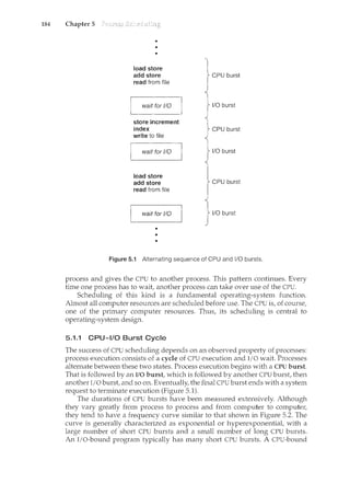
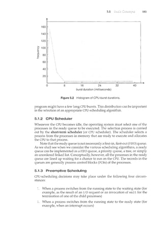
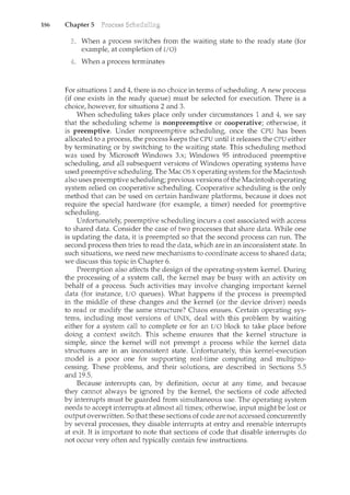
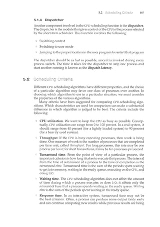
![188 Chapter 5
5.3
output to the user. Thus, another measure is the time from the submission
of a request until the first response is produced. This measure, called
response time, is the tince it takes to start responding, not the time it takes
to output the response. The turnaround time is generally limited by the
speed of the output device.
It is desirable to maximize CPU utilization and throughput and to minirnize
turnaround time, waiting time, and response time. In most cases, we optimize
the average measure. However, under some circumstances, it is desirable
to optimize the minimum or maximum values rather than the average. For
example, to guarantee that all users get good service, we may want to minirnize
the maximum response time.
Investigators have suggested that, for interactive systems (such as time-
sharing systerns), it is more important to minimize the variance in the response
time than to minimize the average response time. A system with reasonable
and predictable response time may be considered more desirable than a system
that is faster on the average but is highly variable. Howeve1~ little work has
been done on CPU-scheduling algorithms that minimize variance.
As we discuss various CPU-scheduling algorithms in the following section,
we illustrate their operation. An accurate illustration should involve many
processes, each a sequence of several hundred CPU bursts and I/O bursts.
For simplicity, though, we consider only one CPU burst (in milliseconds) per
process in our examples. Our measure of comparison is the average waiting
time. More elaborate evaluation mechanisms are discussed in Section 5.7.
CPU scheduling deals with the problem of deciding which of the processes in the
ready queue is to be allocated the CPU. There are many different CPU-scheduling
algorithms. In this section, we describe several of them.
5.3.1 First-Come, First-Served Scheduling
By far the simplest CPU-scheduling algorithm is the first-come, first-served
(FCFS) scheduling algorithm. With this scheme, the process that requests the
CPU first is allocated the CPU first. The implementation of the FCFS policy is
easily managed with a FIFO queue. When a process enters the ready queue, its
PCB is linked onto the tail of the queue. When the CPU is free, it is allocated to
the process at the head of the queue. The running process is then removed from
the queue. The code for FCFS scheduling is simple to write and understand.
On the negative side, the average waiting time under the FCFS policy is
often quite long. Consider the following set of processes that arrive at time 0,
with the length of the CPU burst given in milliseconds:
Process Burst Time
- - - - -
p] 24
p2 3
Po
:) 3](https://image.slidesharecdn.com/elecnwintjql7eggtsqw-operating-system-concepts-8th-editiona4-230117160154-4fa44b38/85/Operating_System_Concepts_8th_EditionA4-pdf-202-320.jpg)
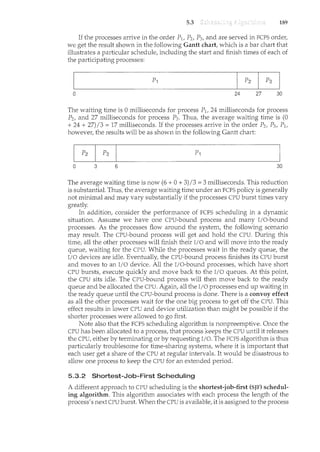
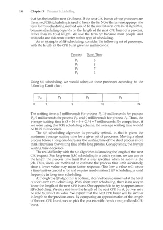
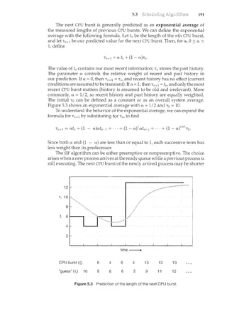
![192 Chapter 5
than what is left of the currently executing process. A preemptive SJF algorithm
will preempt the currently executing process, whereas a nonpreemptive SJF
algorithm will allow the currently running process to finish its CPU burst.
Preemptive SJF scheduling is sometimes called shortest-remaining-time-first
scheduling.
As an example, consider the following four processes, with the length of
the CPU burst given in milliseconds:
Process Arrival Time Burst Time
pl 0 8
p2 1 4
p3 2 9
p4 3 5
If the processes arrive at the ready queue at the times shown and need the
indicated burst times, then the resulting preemptive SJF schedule is as depicted
in the following Gantt chart:
0 5 10 17 26
Process P1 is started at time 0, since it is the only process in the queue. Process
P2 arrives at time 1. The remaining time for process P1 (7 milliseconds) is
larger than the time required by process P2 (4 milliseconds), so process P1 is
preempted, and process P2 is scheduled. The average waiting time for this
example is [(10- 1) + (1 - 1) + (17- 2) +(5-3)]/4 = 26/4 = 6.5 milliseconds.
Nonpreemptive SJF scheduling would result in an average waiting time of 7.75
milliseconds.
5.3.3 Priority Scheduling
The SJF algorithm is a special case of the general priority scheduling algorithm.
A priority is associated with each process, and the CPU is allocated to the process
with the highest priority. Equal-priority processes are scheduled in FCFS order.
An SJF algorithm is simply a priority algorithm where the priority (p) is the
inverse of the (predicted) next CPU burst. The larger the CPU burst, the lower
the priority, and vice versa.
Note that we discuss scheduling in terms of high priority and low priority.
Priorities are generally indicated by some fixed range of numbers, such as 0
to 7 or 0 to 4,095. However, there is no general agreement on whether 0 is the
highest or lowest priority. Some systems use low numbers to represent low
priority; others use low numbers for high priority. This difference can lead to
confusion. In this text, we assume that low numbers represent high priority.
As an example, consider the following set of processes, assumed to have
arrived at time 0 in the order P1, P2, · · ·, Ps, with the length of the CPU burst
given in milliseconds:](https://image.slidesharecdn.com/elecnwintjql7eggtsqw-operating-system-concepts-8th-editiona4-230117160154-4fa44b38/85/Operating_System_Concepts_8th_EditionA4-pdf-206-320.jpg)
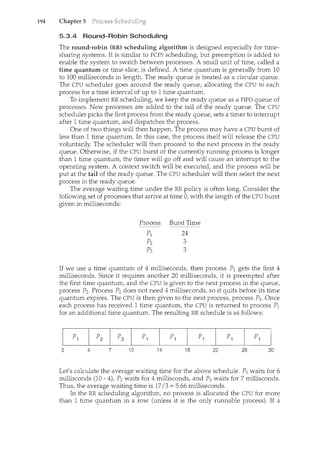
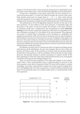
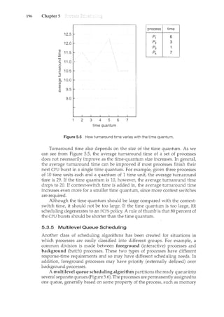
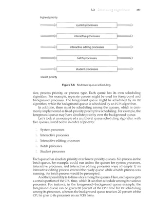
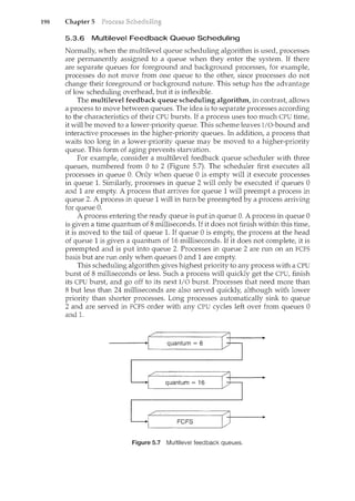
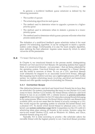
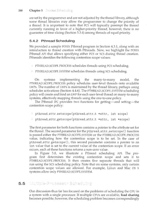
![505
#include <pthreadoh>
#include <stdiooh>
#define NUM_THREADS 5
int main(int argc, char *argv[])
{
}
int i, scope;
pthread_t tid[NUM_THREADS];
pthread_attr_t attr;
I* get the default attributes *I
pthread_attr_init(&attr);
I* first inquire on the current scope *I
if (pthread_attr_getscope(&attr, &scope) != 0)
fprintf(stderr, "Unable to get scheduling scopen");
else {
}
if (scope == PTHREAD_SCOPE_PROCESS)
printf("PTHREAD_SCOPLPROCESS");
else if (scope == PTHREAD_SCOPE_SYSTEM)
printf("PTHREAD_SCOPE_SYSTEM");
else
fprintf(stderr, "Illegal scope valueon");
I* set the scheduling algorithm to PCS or SCS *I
pthread_attr_setscope(&attr, PTHREAD_SCOPE_SYSTEM);
I* create the threads *I
for (i = 0; i < NUM_THREADS; i++)
pthread_create(&tid[i] ,&attr,runner,NULL);
I* now join on each thread *I
for (i = 0; i < NUM_THREADS; i++)
pthread_join(tid[i], NULL);
I* Each thread will begin control in this function *I
void *runner(void *param)
{
I* do some work 000 *I
pthread_exit (0) ;
}
Figure 508 Pthread scheduling API.
201
more complex. Many possibilities have been tried; and as we saw with single-
processor CPU scheduling, there is no one best solution. Here, we discuss
several concerns in multiprocessor scheduling. We concentrate on systems](https://image.slidesharecdn.com/elecnwintjql7eggtsqw-operating-system-concepts-8th-editiona4-230117160154-4fa44b38/85/Operating_System_Concepts_8th_EditionA4-pdf-215-320.jpg)
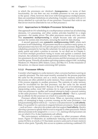
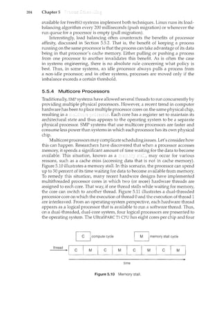
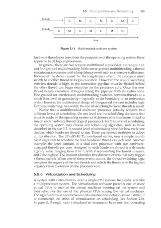
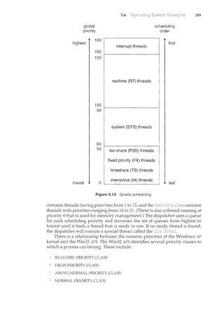

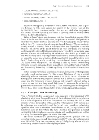
![212 Chapter 5
numeric
priority
0
99
100
140
relative
priority
highest
lowest
time
quantum
200 ms
10 ms
Figure 5.15 The relationship between priorities and time-slice length.
Unlike schedulers for many other systems, including Solaris (Section 5.6.1)
and Windows XP (Section 5.6.2), Lim1X assigns higher-priority tasks longer time
quanta and lower-priority tasks shorter time quanta. The relationship between
priorities and tim.e-slice length is shown in Figure 5.15.
A runnable task is considered eligible for execution on the CPU as long
as it has time remaining in its time slice. When a task has exhausted its time
slice, it is considered expired and is not eligible for execution again until all
other tasks have also exhausted their time quanta. The kernel maintains a list
of all runnable tasks in a data structure. Because of its support for
SMP, each processor maintains its own nmqueue and schedules itself indepen-
dently. Each runqueue contains two priority arrays: and The
active array contains all tasks with time remaining in their time slices, and the
expired array contains all expired tasks. Each of these priority arrays contains a
list of tasks indexed according to priority (Figure 5.16). The scheduler chooses
the task with the highest priority from the active array for execution on the
CPU. On multiprocessor machines, this means that each processor is scheduling
the highest-priority task from its own runqueue structure. When all tasks have
exhausted their time slices (that is, the active array is empty), the two priority
arrays are exchanged; the expired array becomes the active array, and vice
versa.
Linux implements real-time scheduling as defined by POSIX.1b, which is
described in Section 5.4.2. Real-time tasks are assigned static priorities. All
active
array
priority
[0]
[1]
[140]
task lists
o-o
0--0--0
0
expired
array
priority
[0]
[1]
•
[140]
task lists
o--o-o
0
Figure 5.16 List of tasks indexed according to priority.](https://image.slidesharecdn.com/elecnwintjql7eggtsqw-operating-system-concepts-8th-editiona4-230117160154-4fa44b38/85/Operating_System_Concepts_8th_EditionA4-pdf-226-320.jpg)
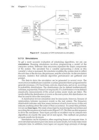
![222 Chapter 5
decisions on the information you have at the time the decision must be
made.
Process Arrival Time Burst Time
- - - - - -
pl 0.0 8
p2 0.4 4
p3 1.0 1
a. What is the average turnaround time for these processes with the
FCFS scheduling algorithm?
b. What is the average turnaround time for these processes with the
SJF scheduling algorithm?
c. The SJF algorithm is supposed to improve performance, but notice
that we chose to run process P1 at time 0 because we did not k11ow
that two shorter processes would arrive soon. Compute what the
average turnaround time will be if the CPU is left idle for the first
1 unit and then SJF scheduling is used. Remember that processes
P1 and P2 are waiting durirtg this idle time, so their waiting time
may increase. This algorithm could be known as future-knowledge
scheduling.
Feedback queues were originally implemented on the CTSS system described
in Corbato et al. [1962]. This feedback queue scheduling system was analyzed
by Schrage [1967]. The preemptive priority scheduling algorithm of Exercise
5.16 was suggested by Kleinrock [1975].
Anderson et al. [1989], Lewis and Berg [1998], and Philbin et al. [1996]
discuss thread scheduling. Multicore scheduling is examined in McNairy and
Bhatia [2005] and Kongetira et al. [2005].
Scheduling techniques that take into account information regarding pro-
cess execution times from previous runs are described in Fisher [1981], Hall
et al. [1996], and Lowney et al. [1993].
Fair-share schedulers are covered by Henry [1984], Woodside [1986], and
Kay and La·uder [1988].
Scheduling policies used in the UNIX V operating system are described
by Bach [1987]; those for UNIX FreeBSD 5.2 are presented by McKusick and
Neville-Neil [2005]; and those for the Mach operating system are discussed
by Black [1990]. Love [2005] covers scheduling in Lim.IX. Details of the ULE
scheduler can be found in Roberson [2003]. Solaris scheduling is described
by Mauro and McDougall [2007]. Solomon [1998], Solomon and Russinovich
[2000], and Russinovich and Solomon [2005] discuss scheduling in Windows
internals. Butenhof [1997] and Lewis and Berg [1998] describe scheduling
in Pthreads systems. Siddha et al. [2007] discuss scheduling challenges on
multicore systems.](https://image.slidesharecdn.com/elecnwintjql7eggtsqw-operating-system-concepts-8th-editiona4-230117160154-4fa44b38/85/Operating_System_Concepts_8th_EditionA4-pdf-236-320.jpg)


![226 Chapter 6
decremented every time we remove one item from the buffer. The code for the
producer process can be modified as follows:
while (true) {
}
I* produce an item in nextProduced *I
while (counter == BUFFER_SIZE)
; I* do nothing *I
buffer[in] = nextProduced;
in = (in + 1) % BUFFER_SIZE ;
counter++;
The code for the consumer process can be modified as follows:
while (true) {
}
while (counter == 0)
; I* do nothing *I
nextConsumed = buffer[out];
out = (out + 1) % BUFFER_SIZE;
counter--;
I* consume the item in nextConsumed *I
Although both the producer and consumer routines shown above are
correct separately, they may not function correctly when executed concurrently.
As an illustration, suppose that the value of the variable counter is currently
5 and that the producer and consumer processes execute the statements
"counter++" and "counter--" concurrently. Following the execution of these
two statements, the value of the variable counter may be 4, 5, or 6! The only
correct result, though, is counter == 5, which is generated correctly if the
producer and consumer execute separately.
We can show that the value of counter may be incorrect as follows. Note
that the statement"counter++" may be implemented in machine language (on
a typical machine) as
register1= counter
register1=register1+ 1
counter= register1
where register1 is one of the local CPU registers. Similarly, the statement
register2"counter--" is implemented as follows:
register2= counter
register2=register2 ~ 1
counter= register2
where again register2is on eo£ the local CPU registers. Even though register1and
register2 may be the same physical register (an accumulator, say), remember
that the contents of this register will be saved and restored by the interrupt
handler (Section 1.2.3).](https://image.slidesharecdn.com/elecnwintjql7eggtsqw-operating-system-concepts-8th-editiona4-230117160154-4fa44b38/85/Operating_System_Concepts_8th_EditionA4-pdf-240-320.jpg)
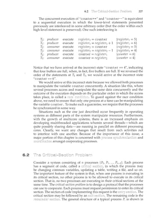
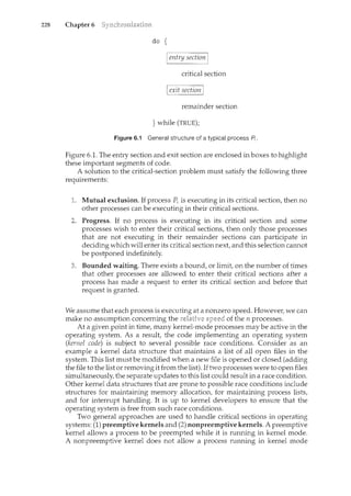
![6.3
6.3 229
to be preempted; a kernel-mode process will run until it exits kernel mode,
blocks, or voluntarily yields control of the CPU. Obviously, a nonpreemptive
kernel is essentially free from race conditions on kernel data structures, as only
one process is active in the kernel at a time. We cannot say the same about
preemptive kernels, so they must be carefully designed to ensure that shared
kernel data are free from race conditions. Preemptive kernels are especially
difficult to design for SMP architectures, since in these environments it is
possible for two kernel-mode processes to run simultaneously on different
processors.
Why, then, would anyone favor a preemptive kernel over a nonpreemptive
one? A preemptive kernel is more suitable for real-time programming, as it will
allow a real-time process to preempt a process currently running in the kernel.
Furthermore, a preemptive kernel may be more responsive, since there is less
risk that a kernel-mode process will run for an arbitrarily long period before
relinquishing the processor to waiting processes. Of course, this effect can be
minimized by designing kernel code that does not behave in this way. Later in
this chapter, we explore how various operating systems manage preemption
within the kernel.
Next, we illustrate a classic software-based solution to the critical-section
problem known as Peterson's solution. Because of the way modern computer
architectures perform basic machine-language instructions, such as load and
store, there are no guarantees that Peterson's solution will work correctly on
such architectures. Howeve1~ we present the solutionbecause it provides a good
algorithmic description of solving the critical-section problem and illustrates
some of the complexities involved in designing software that addresses the
requirements of mutual exclusion, progress, and bomcded waiting.
Peterson's solution is restricted to two processes that alternate execution
between their critical sections and remainder sections. The processes are
numbered Po and P1. For convenience, when presenting Pi, we use Pj to
denote the other process; that is, j equals 1 - i.
Peterson's solution requires the two processes to share two data items:
int turn;
boolean flag[2];
The variable turn indicates whose turn it is to enter its critical section. That is,
if turn == i, then process Pi is allowed to execute in its critical section. The
flag array is used to indicate if a process is ready to enter its critical section.
For example, if flag [i] is true, this value indicates that Pi is ready to enter
its critical section. With an explanation of these data structures complete, we
are now ready to describe the algorithm shown in Figure 6.2.
To enter the critical section, process Pi first sets flag [i] to be true and
then sets turn to the value j, thereby asserting that if the other process wishes
to enter the critical section, it can do so. If both processes try to enter at the same
time, turn will be set to both i and j at roughly the sance time. Only one of these
assignments will last; the other will occur but will be overwritten immediately.](https://image.slidesharecdn.com/elecnwintjql7eggtsqw-operating-system-concepts-8th-editiona4-230117160154-4fa44b38/85/Operating_System_Concepts_8th_EditionA4-pdf-243-320.jpg)
![230 Chapter 6
do {
flag [i] = TRUE;
turn= j;
while (flag[j] && turn j);
critical section
I flag [i] = FALSE; I
remainder section
} while (TRUE);
Figure 6.2 The structure of process A in Peterson's solution.
The eventual value of turn determines which of the two processes is allowed
to enter its critical section first.
We now prove that this solution is correct. We need to show that:
Mutual exclusion is preserved.
The progress requirement is satisfied.
The bounded-waiting requirement is met.
To prove property 1, we note that each P; enters its critical section only
if either flag [j] == false or turn == i. Also note that, if both processes
can be executing in their critical sections at the same time, then flag [0] ==
flag [1] ==true. These two observations imply that Po and P1 could not have
successfully executed their while statements at about the same time, since the
value of turn canbe either 0 or 1but camwt be both. Hence, one of the processes
-say, Pi -must have successfully executed the while statencent, whereas P;
had to execute at least one additional statement ("turn== j"). However, at
that time, flag [j] == true and turn == j, and this condition will persist as
long as Pi is in its critical section; as a result, mutual exclusion is preserved.
To prove properties 2 and 3, we note that a process P; can be prevented from
entering the critical section only if it is stuck in the while loop with the condition
flag [j] ==true and turn=== j; this loop is the only one possible. If Pi is not
ready to enter the critical section, then flag [j] ==false, and P; can enter its
critical section. If Pj has set flag [j] to true and is also executing in its while
statement, then either turn === i or turn === j. If turn == i, then P; will enter
the critical section. If turn== j, then Pi will enter the critical section. However,
once Pi exits its critical section, it will reset flag [j] to false, allowing P; to
enter its critical section. If Pi resets flag [j] to true, it must also set turn to i.
Thus, since P; does not change the value of the variable turn while executing
the while statement, P; will enter the critical section (progress) after at most
one entry by P1 (bounded waiting).](https://image.slidesharecdn.com/elecnwintjql7eggtsqw-operating-system-concepts-8th-editiona4-230117160154-4fa44b38/85/Operating_System_Concepts_8th_EditionA4-pdf-244-320.jpg)
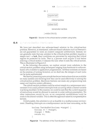
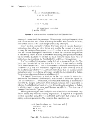
![6.4
do {
key = TRUE;
while (key == TRUE)
Swap(&lock, &key);
II critical section
lock = FALSE;
II remainder section
} while (TRUE);
Figure 6.7 Mutual-exclusion implementation with the Swap() instruction.
boolean waiting[n];
boolean lock;
233
These data structures are initialized to false. To prove that the mutual-
exclusion requirement is met, we note that process P; can enter its critical
section only if either waiting [i] == false or key == false. The value
of key can become false only if the TestAndSet () is executed. The first
process to execute the TestAndSet () will find key== false; all others must
wait. The variable waiting [i] can become false only if another process
leaves its critical section; only one waiting [i] is set to false, maintaining the
mutual-exclusion requirement.
do {
waiting[i] = TRUE;
key = TRUE;
while (waiting[i] && key)
key= TestAndSet(&lock);
waiting[i] = FALSE;
II critical section
j = (i + 1) %n;
while ((j != i) && !waiting[j])
j = (j + 1) %n;
if (j == i)
lock = FALSE;
else
waiting[j] = FALSE;
II remainder section
} while (TRUE) ;
Figure 6.8 Bounded-waiting mutual exclusion with TestAndSet ().](https://image.slidesharecdn.com/elecnwintjql7eggtsqw-operating-system-concepts-8th-editiona4-230117160154-4fa44b38/85/Operating_System_Concepts_8th_EditionA4-pdf-247-320.jpg)
![234 Chapter 6
6.5
To prove that the progress requirement is met, we note that the arguments
presented for mutual exclusion also apply here, since a process exiting the
critical section either sets lock to false or sets waiting[j] to false. Both
allow a process that is waiting to enter its critical section to proceed.
To prove that the bounded-waiting requirement is met, we note that, when
a process leaves its critical section, it scans the array waiting in the cyclic
ordering (i + 1, i + 2, ..., n 1, 0, ..., i 1). It designates the first process in this
ordering that is in the entry section (waiting[j] ==true) as the next one to
enter the critical section. Any process waiting to enter its critical section will
thus do so within n - 1 turns.
Unfortunately for hardware designers, implementing atomic TestAnd-
Set () instructions on multiprocessors is not a trivial task. Such implementa-
tions are discussed in books on computer architecture.
The hardware-based solutions to the critical-section problem presented in
Section 6.4 are complicated for application programmers to use. To overcmrte
this difficulty, we can use a synchronization tool called a
A semaphore S is an integer variable that, apart from initialization, is
accessed only through two standard atomic operations: wait () and signal ().
The wait () operation was originally termed P (from the Dutch proberen, "to
test"); signal() was originally called V (from verhogen, "to increment"). The
definition of wait () is as follows:
wait(S) {
}
while S <= 0
II no-op
s--·'
The definition of signal() is as follows:
signal(S) {
S++;
}
All modifications to the integer value of the semaphore in the wait () and
signal() operations must be executed indivisibly. That is, when one process
modifies the semaphore value, no other process can simultaneously modify
that same semaphore value. In addition, in the case of wait (S), the testing of
the integer value of S (S :S 0), as well as its possible modification (S--), must
be executed without interruption. We shall see how these operations can be
implemented in Section 6.5.2; first, let us see how semaphores can be used.
6.5.1 Usage
Operating systems often distinguish between counting and binary semaphores.
The value of a counting semaphore can range over an unrestricted domain.
The value of a binary semaphore can range only between 0 and 1. On some](https://image.slidesharecdn.com/elecnwintjql7eggtsqw-operating-system-concepts-8th-editiona4-230117160154-4fa44b38/85/Operating_System_Concepts_8th_EditionA4-pdf-248-320.jpg)
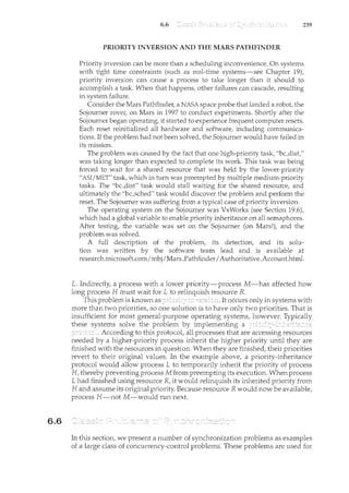
![6.6 243
Figure 6.14 The situation of the dining philosophers.
to one philosopher. In the center of the table is a bowl of rice, and the table is laid
with five single chopsticks (Figure 6.14). When a philosopher thinks, she does
not interact with her colleagues. From time to time, a philosopher gets hungry
and tries to pick up the two chopsticks that are closest to her (the chopsticks
that are between her and her left and right neighbors). A philosopher may pick
up only one chopstick at a time. Obviously, she cam1ot pick up a chopstick that
is already in the hand of a neighbor. When a htmgry philosopher has both her
chopsticks at the same time, she eats without releasing her chopsticks. When
she is finished eating, she puts down both of her chopsticks and starts thinking
again.
The dining-philosophers problem is considered a classic synchronization
problem neither because of its practical importance nor because computer
scientists dislike philosophers but because it is an example of a large class
of concurrency-control problems. It is a simple representation of the need
to allocate several resources among several processes in a deadlock-free and
starvation-free mam1er.
One simple solution is to represent each chopstick with a semaphore. A
philosopher tries to grab a chopstick by executing await () operation on that
semaphore; she releases her chopsticks by executing the signal() operation
on the appropriate semaphores. Thus, the shared data are
semaphore chopstick[5];
where all the elements of chopstick are initialized to 1. The structure of
philosopher i is shown in Figure 6.15.
Although this solution guarantees that no two neighbors are eating
simultaneously, it nevertheless must be rejected because it could create a
deadlock. Suppose that all five philosophers become hungry simultaneously
and each grabs her left chopstick. All the elements of chopstick will now be
equal to 0. When each philosopher tries to grab her right chopstick, she will be
delayed forever.
Several possible remedies to the deadlock problem are listed next.
Allow at most four philosophers to be sitting simultaneously at the table.](https://image.slidesharecdn.com/elecnwintjql7eggtsqw-operating-system-concepts-8th-editiona4-230117160154-4fa44b38/85/Operating_System_Concepts_8th_EditionA4-pdf-257-320.jpg)
![244 Chapter 6
6.7
do {
wait(chopstick[i]);
wait(chopstick[(i+l) %5]);
I I eat
signal(chopstick[i]);
signal(chopstick[(i+l) %5]);
II think
} while (TRUE);
Figure 6.15 The structure of philosopher i.
Allow a philosopher to pick up her chopsticks only if both chopsticks are
available (to do this, she must pick them up in a critical section).
Use an asymmetric solution; that is, an odd philosopher picks up first her
left chopstick and then her right chopstick, whereas an even philosopher
picks up her right chopstick and then her left chopstick
In Section 6.7, we present a solution to the dining-philosophers problem
that ensures freedom from deadlocks. Note, however, that any satisfactory
solution to the dining-philosophers problem must guard against the possibility
that one of the philosophers will starve to death. A deadlock-free solution does
not necessarily eliminate the possibility of starvation.
Although semaphores provide a convenient and effective mechanism for
process synchronization, using them incorrectly can result in timing errors
that are difficult to detect, since these errors happen only if some particular
execution sequences take place and these sequences do not always occur.
We have seen an example of such errors in the use of counters in our
solution to the producer-consumer problem (Section 6.1). In that example,
the timing problem happened only rarely, and even then the counter value
appeared to be reasonable-off by only 1. Nevertheless, the solution is
obviously not an acceptable one. It is for this reason that semaphores were
introduced in the first place.
Unfortunately, such timing errors can still occur when semaphores are
used. To illustrate how, we review the semaphore solution to the critical-section
problem. All processes share a semaphore variable mutex, which is initialized
to 1. Each process must execute wait (mutex) before entering the critical section
and signal (mutex) afterward. If this sequence is not observed, two processes
may be in their critical sections simultaneously. Next, we examine the various
difficulties that may result. Note that these difficulties will arise even if a
single process is not well behaved. This situation may be caused by an honest
programming error or an uncooperative programmer.](https://image.slidesharecdn.com/elecnwintjql7eggtsqw-operating-system-concepts-8th-editiona4-230117160154-4fa44b38/85/Operating_System_Concepts_8th_EditionA4-pdf-258-320.jpg)
![248 Chapter 6
queues associated with {
x, y conditions ;-_:__----~-~-------
...
operations
initialization
code
Figure 6.18 Monitor with condition variables.
6.7.2 Dining-Philosophers Solution Using Monitors
Next, we illustrate monitor concepts by presenting a deadlock-free solution to
the dining-philosophers problem. This solution imposes the restriction that a
philosopher may pick up her chopsticks only if both of them are available. To
code this solution, we need to distinguish among three states in which we may
find a philosopher. For this purpose, we introduce the following data structure:
enum{THINKING, HUNGRY, EATING}state[5];
Philosopher i can set the variable state [i] = EATING only if her two
neighbors are not eating: (state [ (i+4) % 5] ! = EATING) and (state [ (i+1)
% 5] '= EATING).
We also need to declare
condition sel£[5];
in which philosopher i can delay herself when she is hungry but is unable to
obtain the chopsticks she needs.
We are now in a position to describe our solution to the dining-philosophers
problem. The distribution of the chopsticks is controlled by the monitor Din-
ingPhilosophers, whose definition is shown in Figure 6.19. Each philosopher,
before starting to eat, must invoke the operation pickup(). This act n'lay result
in the suspension of the philosopher process. After the successful completion of
the operation, the philosopher may eat. Following this, the philosopher invokes](https://image.slidesharecdn.com/elecnwintjql7eggtsqw-operating-system-concepts-8th-editiona4-230117160154-4fa44b38/85/Operating_System_Concepts_8th_EditionA4-pdf-262-320.jpg)
![6.7
monitor dp
{
}
enum {THINKING, HUNGRY, EATING} state[5];
condition self[5];
void pickup(int i) {
state[i] =HUNGRY;
test(i);
}
if (state [i] ! = EATING)
self [i] .wait() ;
void putdown(int i) {
state[i] =THINKING;
test((i + 4) %5);
test((i + 1) %5);
}
void test(int i) {
}
if ((state[(i + 4) % 5] !=EATING) &&
(state[i] ==HUNGRY) &&
}
(state[(i + 1) % 5] !=EATING)) {
state[i] =EATING;
self[i] .signal();
initialization_code() {
}
for (int i = 0; i < 5; i++)
state[i] =THINKING;
Figure 6.19 A monitor solution to the dining-philosopher problem.
249
the putdown() operation. Thus, philosopher i must invoke the operations
pickup() and putdown() in the following sequence:
DiningPhilosophers.pickup(i);
eat
DiningPhilosophers.putdown(i);
It is easy to show that this solution ensures that no two neighbors are eating
simultaneously and that no deadlocks will occur. We note, however, that it is
possible for a philosopher to starve to death. We do not present a solution to
this problem but rather leave it as an exercise for you.](https://image.slidesharecdn.com/elecnwintjql7eggtsqw-operating-system-concepts-8th-editiona4-230117160154-4fa44b38/85/Operating_System_Concepts_8th_EditionA4-pdf-263-320.jpg)
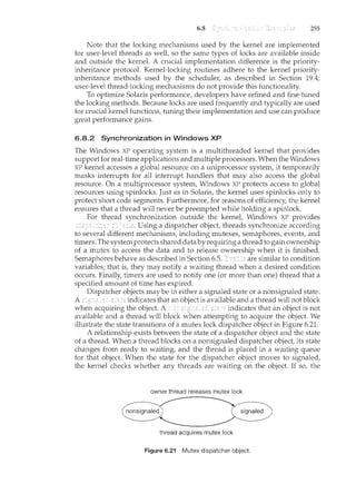
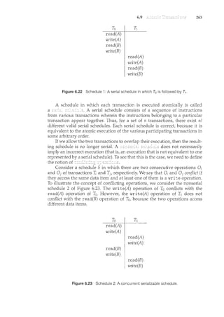
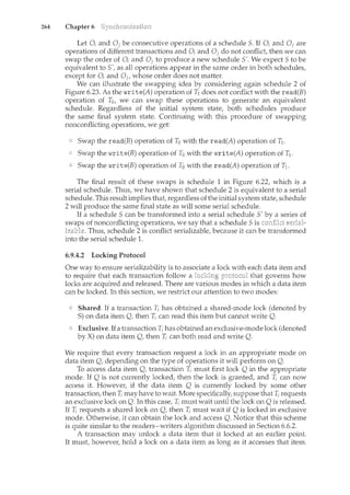
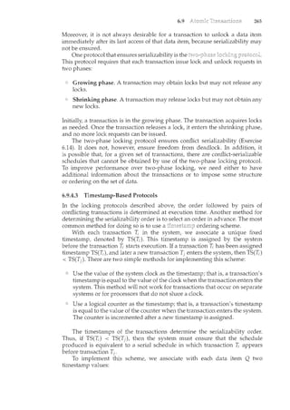
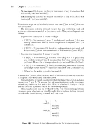
![6.10
267
The timestamp protocol ensures conflict serializability. This capability
follows from the fact that conflicting operations are processed in timestamp
order. The protocol also ensures freedom fron1 deadlocl<:, because no transaction
ever waits.
Given a collection of cooperating sequential processes that share data, mutual
exclusion must be provided to ensure that a critical section of code is used
by only one process or thread at a tince. Typically, computer hardware
provides several operations that ensure mutual exclusion. However, such
hardware-based solutions are too complicated for most developers to use.
Semaphores overcome this obstacle. Semaphores can be used to solve various
synchronization problems and can be implemented efficiently, especially if
hardware support for atomic operations is available.
Various synchronization problems (such as the bounded-buffer problem,
the readers-writers problem, and the dining-philosophers problem) are impor-
tant mainly because they are examples of a large class of concurrency-control
problems. These problems are used to test nearly every newly proposed
synchronization scheme.
The operating system must provide the means to guard against timing
errors. Several language constructs have been proposed to deal with these prob-
lems. Monitors provide the synchronization mechanism for sharing abstract
data types. A condition variable provides a method by which a monitor
procedure can block its execution until it is signaled to continue.
Operating systems also provide support for synchronization. For example,
Solaris, Windows XP, and Linux provide mechanisms such as semaphores,
mutexes, spinlocks, and condition variables to control access to shared data.
The Pthreads API provides support for mutexes and condition variables.
A transaction is a program unit that must be executed atomically; that
is, either all the operations associated with it are executed to completion, or
none are performed. To ensure atomicity despite system failure, we can use a
write-ahead log. All updates are recorded on the log, which is kept in stable
storage. If a system crash occurs, the information in the log is used in restoring
the state of the updated data items, which is accomplished by use of the undo
and redo operations. To reduce the overhead in searching the log after a system
failure has occurred, we can use a checkpoint scheme.
To ensure serializability when the execution of several transactions over-
laps, we must use a concurrency-control scheme. Various concurrency-control
schemes ensure serializability by delaying an operation or aborting the trans-
action that issued the operation. The most common ones are locking protocols
and timestamp ordering schemes.
6.1 The first known correct software sohJtion to the critical-section problem
for two processes was developed by Dekker. The two processes, P0 and
P1, share the following variables:
boolean flag[2]; I* initially false *I
int turn;](https://image.slidesharecdn.com/elecnwintjql7eggtsqw-operating-system-concepts-8th-editiona4-230117160154-4fa44b38/85/Operating_System_Concepts_8th_EditionA4-pdf-281-320.jpg)
![268 Chapter 6
do {
flag[i] = TRUE;
while (flag[j]) {
}
if (turn == j) {
flag [i] = false;
while (turn == j)
; II do nothing
flag [i] = TRUE;
}
II critical section
turn= j;
flag [i] = FALSE;
II remainder section
} while (TRUE);
Figure 6.25 The structure of process A in Dekker's algorithm.
The structure of process Pi (i == 0 or 1) is shown in Figure 6.25; the other
process is P1 (j == 1 or 0). Prove that the algorithm satisfies all three
requirements for the critical-section problem.
6.2 Explain why interrupts are not appropriate for implementing synchro-
nization primitives in multiprocessor systems.
6.3 The first known correct software solution to the critical-section problem
for n processes with a lower bound on waiting of n - 1 turns was
presented by Eisenberg and McGuire. The processes share the following
variables:
enum pstate {idle, want_in, in_cs};
pstate flag [n] ;
int turn;
All the elements of flag are initially idle; the initial value of turn is
immaterial (between 0 and n-1). The structure of process Pi is shown in
Figure 6.26. Prove that the algorithm satisfies all three requiren'lents for
the critical-section problem.
6.4 Write a monitor that implements an alarm clock that enables a calling
program to delay itself for a specified number of tirne units (ticks).
You may assume the existence of a real hardware clock that invokes
a procedure hclc in your monitor at regular intervals.
6.5 A file is to be shared among different processes, each of which has
a unique number. The file can be accessed simultaneously by several
processes, subject to the following constraint: The sum of all unique](https://image.slidesharecdn.com/elecnwintjql7eggtsqw-operating-system-concepts-8th-editiona4-230117160154-4fa44b38/85/Operating_System_Concepts_8th_EditionA4-pdf-282-320.jpg)
![do {
while (TRUE) {
flag[i] = want_in;
j = turn;
}
while (j != i) {
}
if (flag [j] I= idle) {
j = turn;
else
j = (j + 1) %n;
flag [i]
j = 0;
in_cs;
while ( (j < n) && (j
j++;
if ( (j >= n) && (turn
break;
II critical section
j = (turn + 1) %n;
while (flag[j] == idle)
j = (j + 1) %n;
turn= j;
flag [i] = idle;
II remainder section
} while (TRUE);
i II flag[j] != in_cs))
i I I flag [turn] idle))
Figure 6.26 The structure of process A in Eisenberg and McGuire's algorithm.
269
numbers associated with all the processes currently accessing the file
must be less than n. Write a monitor to coordinate access to the file.
6.6 The decrease_count () function in the previous exercise currently
returns 0 if sufficient resources are available and -1 otherwise. This
leads to awkward programming for a process that wishes to obtain a
number of resources:
while (decrease_count(count) == -1)
Rewrite the resource-manager code segment using a monitor and
condition variables so that the decrease_count () function suspends](https://image.slidesharecdn.com/elecnwintjql7eggtsqw-operating-system-concepts-8th-editiona4-230117160154-4fa44b38/85/Operating_System_Concepts_8th_EditionA4-pdf-283-320.jpg)
![270 Chapter 6
the process until sufficient resources are available. This will allow a
process to invoke decrease_count () by simply calling
decrease_count(count);
The process will return from this function call only when sufficient
resources are available.
6.7 Exercise 4.12 requires the parent thread to wait for the child thread to
finish its execution before printing out the computed values. If we let
the parent thread access the Fibonacci numbers as soon as they have
been computed by the child thread - rather than waiting for the child
thread to terminate- Explain what changes would be necessary to the
solution for this exercise? Implement your modified solution.
6.8 In Section 6.4, we mentioned that disabling interrupts frequently can
affect the system's clock. Explain why this can occur and how such
effects can be mil1.imized.
6.9 Servers can be designed to limit the number of open coru1.ections. For
example, a server may wish to have only N socket com1.ections at any
point in time. As soon as N connections are made, the server will
not accept another incoming connection until an existing connection
is released. Explain how semaphores can be used by a server to limit the
number of concurrent connections.
6.10 Why do Solaris, Lil1.ux, and Windows XP use spinlocks as a syn-
chronization mechanism only on multiprocessor systems and not on
single-processor systems?
6.11 Show that, if the wait () and signal () semaphore operations are not
executed atomically, then mutual exclusion may be violated.
6.12 Show how to implement the wait() and signal() semaphore opera-
tions in multiprocessor environments using the TestAndSet () instruc-
tion. The solution should exhibit minimal busy waiting.
6.13 Suppose we replace the wait() and signal() operations of moni-
tors with a single construct await (B), where B is a general Boolean
expression that causes the process executing it to wait until B becomes
true.
a. Write a monitor using this scheme to implement the readers-
writers problem.
b. Explain why, in general, this construct cannot be implemented
efficiently.
c. What restrictions need to be put on the await statement so that it
can be implemented efficiently? (Hint: Restrict the generality of B;
see Kessels [1977].)](https://image.slidesharecdn.com/elecnwintjql7eggtsqw-operating-system-concepts-8th-editiona4-230117160154-4fa44b38/85/Operating_System_Concepts_8th_EditionA4-pdf-284-320.jpg)
![#include "buffer.h"
I* the buffer *I
buffer_item buffer[BUFFER_SIZE];
int insert_item(buffer_item item) {
I* insert item into buffer
return 0 if successful, otherwise
return -1 indicating an error condition *I
}
int remove_item(buffer_item *item) {
}
I* remove an object from buffer
placing it in item
return 0 if successful, otherwise
return -1 indicating an error condition *I
Figure 6.27 Askeleton program.
275
The insert_item() and remove_item() functions will synchronize
the producer and consumer using the algorithms outlined in Figures
6.10 and 6.11. The buffer will also require an initialization function that
initializes the mutual-exclusion object mutex along with the empty and
full semaphores.
The main() f-Lmction will initialize the buffer and create the separate
producer and consumer threads. Once it has created the producer
and consumer threads, the main() function will sleep for a period of
time and, upon awakening, will terminate the application. The main ()
function will be passed three parameters on the command line:
a. How long to sleep before terminating
b. The number of producer threads
c. The nuncber of consumer threads
A skeleton for this function appears in Figure 6.28.
#include "buffer.h"
int main(int argc, char *argv[]) {
}
I* 1. Get command line arguments argv[1] ,argv[2] ,argv[3] *I
I* 2. Initialize buffer *I
I* 3. Create producer thread(s) *I
I* 4. Create consumer thread(s) *I
I* 5. Sleep *I
I* 6. Exit *I
Figure 6.28 Askeleton program.](https://image.slidesharecdn.com/elecnwintjql7eggtsqw-operating-system-concepts-8th-editiona4-230117160154-4fa44b38/85/Operating_System_Concepts_8th_EditionA4-pdf-289-320.jpg)
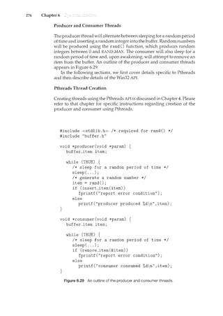
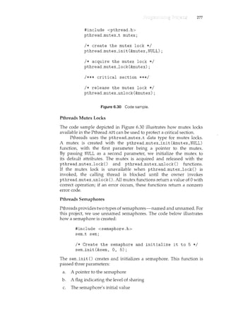
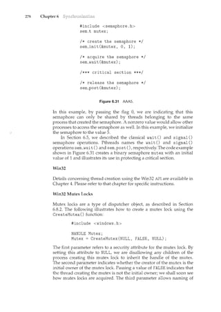
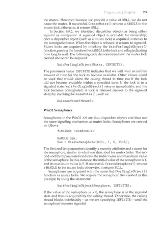
![280 Chapter 6
The equivalent of the signal () operation on Win32 semaphores is the
ReleaseSemaphore () function. This function is passed three parame-
ters:
a. The HANDLE of the semaphore
b. The amount by which to increase the value of the semaphore
c. A pointer to the previous value of the semaphore
We can increase Sem by 1 using the following statement:
ReleaseSemaphore(Sem, 1, ~LL);
Both ReleaseSemaphore () and ReleaseMutex() return nonzero if
successful and zero otherwise.
The mutual-exclusion problem was first discussed in a classic paper by Dijkstra
[1965a]. Dekker's algorithm (Exercise 6.1)-the first correct software solution
to the two-process mutual-exclusion problem-was developed by the Dutch
mathematician T. Dekker. This algorithm also was discussed by Dijkstra
[1965a]. A simpler solution to the two-process mutual-exclusion problem has
since been presented by Peterson [1981] (Figure 6.2).
Dijkstra [1965b] presented the first solution to the mutual-exclusion prob-
lem for n processes. This solution, however, does not have an upper bound on
the amount of time a process must wait before it is allowed to enter the critical
section. Knuth [1966] presented the first algorithm with a bound; his bound
was 211 turns. A refinement of Knuth's algorithm by deBruijn [1967] reduced the
waiting time to n2 turns, after which Eisenberg and McGuire [1972] succeeded
in reducing the time to the lower bound of n-1 turns. Another algorithm
that also requires n-1 turns but is easier to program and to understand is
the bakery algorithm, which was developed by Lamport [1974]. Burns [1978]
developed the hardware-solution algorithm that satisfies the bounded-waiting
requirement.
General discussions concerning the mutual-exclusion problem were
offered by Lamport [1986] and Lamport [1991]. A collection of algorithms for
mutual exclusion was given by Raynal [1986].
The semaphore concept was suggested by Dijkstra [1965a]. Patil [1971]
examined the question of whether semaphores can solve all possible syn-
chronization problems. Parnas [1975] discussed some of the flaws in Patil's
arguments. Kosaraju [1973] followed up on Patil's work to produce a problem
that cannot be solved by wait() and signal() operations. Lipton [1974]
discussed the limitations of various synchronization primitives.
The classic process-coordination problems that we have described are
paradigms for a large class of concurrency-control problems. The bounded-
buffer problem, the dining-philosophers problem, and the sleeping-barber
problem (Exercise 6.36) were suggested by Dijkstra [1965a] and Dijkstra [1971].
The cigarette-smokers problem (Exercise 6.22 was developed by Patil [1971].
The readers-writers problem was suggested by Courtois et al. [1971]. The](https://image.slidesharecdn.com/elecnwintjql7eggtsqw-operating-system-concepts-8th-editiona4-230117160154-4fa44b38/85/Operating_System_Concepts_8th_EditionA4-pdf-294-320.jpg)
![281
issue of concurrent reading and writing was discussed by Lamport [1977].
The problem of synchronization of independent processes was discussed by
Lamport [1976].
The critical-region concept was suggested by Hoare [1972] and by Brinch-
Hansen [1972]. The monitor concept was developed by Brinch-Hansen [1973].
A complete description of the monitor was given by Hoare [1974]. Kessels
[1977] proposed an extension to the monitor to allow automatic signalil1.g.
Experience obtained from the use of monitors in concurrent programs was
discussed by Lampson and Redell [1979]. They also examined the priority
inversion problem. General discussions concerning concurrent programming
were offered by Ben-Ari [1990] and Birrell [1989].
Optimizing the performance of lockil1.g primitives has been discussed in
many works, such as Lamport [1987], Mellor-Crummey and Scott [1991], and
Anderson [1990]. The use of shared objects that do not require the use of critical
sections was discussed in Herlihy [1993], Bershad [1993], and Kopetz and
Reisinger [1993]. Novel hardware instructions and their utility in implementing
synchronization primitives have been described in works such as Culler et al.
[1998], Goodman et al. [1989], Barnes [1993], and Herlihy and Moss [1993].
Some details of the locking mechanisms used in Solaris were presented
in Mauro and McDougall [2007]. Note that the locking mechanisms used by
the kernel are implemented for user-level threads as well, so the same types
of locks are available inside and outside the kernel. Details of Windows 2000
synchronization can be found in Solomon and Russinovich [2000]. Goetz et al.
[2006] presents a detailed discussion of concurrent programming in Java as
well as the java. util. concurrent package.
The write-ahead log scheme was first mtroduced in System Rby Gray et al.
[1981]. The concept of serializability was formulated by Eswaran et al. [1976] in
connectionwith their work on concurrency control for System R. The two-phase
locking protocol was introduced by Eswaran et al. [1976]. The timestamp-
based concurrency-control scheme was provided by Reed [1983]. Various
timestamp-based concurrency-control algorithms were explail1.ed by Bernstem
and Goodman [1980]. Adl-Tabatabai et al. [2007] discusses transactional
memory.](https://image.slidesharecdn.com/elecnwintjql7eggtsqw-operating-system-concepts-8th-editiona4-230117160154-4fa44b38/85/Operating_System_Concepts_8th_EditionA4-pdf-295-320.jpg)

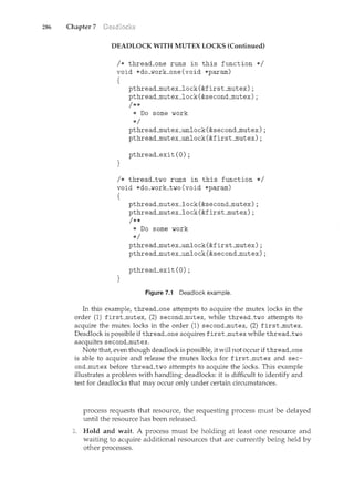
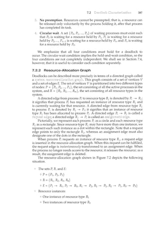
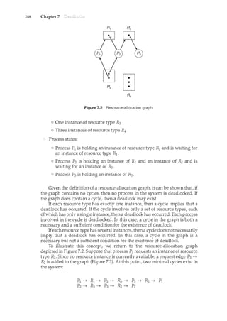
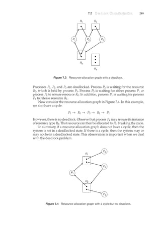
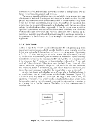
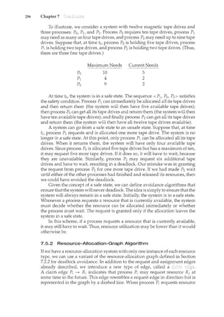
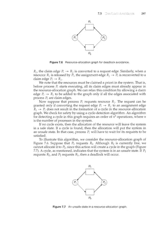
![298 Chapter 7
7.5.3 Banker's Algorithm
The resource-allocation-graph algorithm is not applicable to a resource-
allocation system with multiple instances of each resource type. The deadlock-
avoidance algorithm that we describe next is applicable to such a system but
is less efficient than the resource-allocation graph scheme. This algorithm is
commonly known as the banker's algorithm. The name was chosen because the
algorithm. could be used in a banking system to ensure that the bank never
allocated its available cash in such a way that it could no longer satisfy the
needs of all its customers.
When a new process enters the system, it must declare the maximum
number of instances of each resource type that it may need. This nun1.ber may
not exceed the total number of resources in the system. When a user requests
a set of resources, the system must determine whether the allocation of these
resources will leave the system in a safe state. If it will, the resources are
allocated; otherwise, the process must wait until some other process releases
enough resources.
Several data structures must be maintained to implement the banker's
algorithm. These data structures encode the state of the resource-allocation
system. We need the following data structures, where n is the number of
processes in the system and m is the number of resource types:
Available. A vector of length m indicates the number of available resources
of each type. If Available[j] equals k, then k instances of resource type Ri
are available.
Max. An n x m matrix defines the maximum demand of each process.
If Max[i] [j] equals k, then process P; may request at most k instances of
resource type Ri.
Allocation. An 11 x m matrix defines the number of resources of each type
currently allocated to each process. If Allocation[i][j] equals lc, then process
P; is currently allocated lc instances of resource type Rj.
Need. An n x m matrix indicates the remaining resource need of each
process. If Need[i][j] equals k, then process P; may need k more instances of
resource type Ri to complete its task. Note that Need[i][j] equals Max[i][j]
- Allocation[i][j].
These data structures vary over time in both size and value.
To simplify the presentation of the banker's algorithm, we next establish
some notation. Let X andY be vectors of length 11. We say that X::= Y if and
only if X[i] ::= Y[i] for all i = 1, 2, ..., n. For example, if X = (1,7,3,2) and Y =
(0,3,2,1), then Y ::=X. In addition, Y < X if Y ::=X andY# X.
We can treat each row in the matrices Allocation and Need as vectors
and refer to them as Allocation; and Need;. The vector Allocation; specifies
the resources currently allocated to process P;; the vector Need; specifies the
additional resources that process P; may still request to complete its task.
7.5.3.1 Safety Algorithm
We can now present the algorithm for finding out whether or not a systern is
in a safe state. This algorithm can be described as follows:](https://image.slidesharecdn.com/elecnwintjql7eggtsqw-operating-system-concepts-8th-editiona4-230117160154-4fa44b38/85/Operating_System_Concepts_8th_EditionA4-pdf-312-320.jpg)
![7.5 299
Let Work and Finish be vectors of length m and n, respectively. Initialize
Work= Available and Finish[i] =false for i =0, 1, ... , n - 1.
Find an index i such that both
a. Finish[i] ==false
b. Need; ::; Work
If no such i exists, go to step 4.
Work = Work + Allocation;
Finish[i] = true
Go to step 2.
If Finish[i] ==true for all i, then the system is in a safe state.
This algorithm may require an order of m x n2 operations to determine whether
a state is safe.
7.5.3.2 Resource-Request Algorithm
Next, we describe the algorithm for determining whether requests can be safely
granted.
Let Request; be the request vector for process P;. If Request; [j] == k, then
process P; wants k instances of resource type Rj. When a request for resources
is made by process P;, the following actions are taken:
If Request; ::::; Need;, go to step 2. Otherwise, raise an error condition, since
the process has exceeded its maximum claim.
If Request; ::; Available, go to step 3. Otherwise, P; must wait, since the
resources are not available.
Have the system pretend to have allocated the requested resources to
process P; by modifyil1.g the state as follows:
Available= Available- Request;;
Allocation; =Allocation; +Request;;
Need; =Need;- Request;;
If the resulting resource-allocation state is safe, the transaction is com-
pleted, and process P; is allocated its resources. However, if the new state
is unsafe, then P; must wait for Request;, and the old resource-allocation
state is restored.
7.5.3.3 An Illustrative Example
To illustrate the use of the banker's algorithm, consider a system with five
processes Po through P4 and three resource types A, B, and C. Resource type A
has ten instances, resource type B has five instances, and resource type C has
seven instances. Suppose that, at time T0, the following snapshot of the system
has been taken:](https://image.slidesharecdn.com/elecnwintjql7eggtsqw-operating-system-concepts-8th-editiona4-230117160154-4fa44b38/85/Operating_System_Concepts_8th_EditionA4-pdf-313-320.jpg)
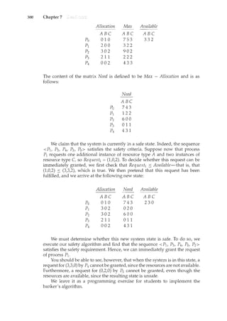
![302 Chapter 7
(a) (b)
Figure 7.8 (a) Resource-allocation graph. (b) Corresponding wait-for graph.
Request. An n x m matrix indicates the current request of each process.
If Request[i][j] equals k, then process P; is requesting k more instances of
resource type Rj.
The:::: relation between two vectors is defined as in Section 7.5.3. To simplify
notation, we again treat the rows in the matrices Allocation and Request as
vectors; we refer to them as Allocation; and Request;. The detection algorithm
described here simply investigates every possible allocation sequence for the
processes that remain to be completed. Compare this algorithm with the
banker's algorithm of Section 7.5.3.
Let Work and Finish be vectors of length m and n, respectively. Initialize
Work= Available. Fori= 0, 1, ..., n-1, if Allocation; # 0, then Finish[i] =false;
otherwise, Finish[i] =tme.
2. Find an index i such that both
a. Finish[i] ==false
b. Request; :::: Work
If no such i exists, go to step 4.
Work= Work+ Allocation;
Finish[i] = true
Go to step 2.
4. If Finish[i] ==false for some i, 0 :::: i < n, then the system is in a deadlocked
state. Moreover, if Finish[i] ==false, then process P; is deadlocked.
This algorithm requires an order o£ m x n2 operations to detect whether the
system is in a deadlocked state.](https://image.slidesharecdn.com/elecnwintjql7eggtsqw-operating-system-concepts-8th-editiona4-230117160154-4fa44b38/85/Operating_System_Concepts_8th_EditionA4-pdf-316-320.jpg)
![7.6 303
You may wonder why we reclaim the resources of process P; (in step 3)
as soon as we determine that Request; :S Work (in step 2b). We know that P;
is currently not involved in a deadlock (since Request; :S Work). Thus, we take
an optimistic attitude and assume that P; will require no more resources to
complete its task; it will thus soon return all currently allocated resources to
the system. If our assumption is incorrect, a deadlock may occur later. That
deadlock will be detected the next tince the deadlock-detection algorithm is
invoked.
To illustrate this algorithm, we consider a system with five processes Po
through P4 and three resource types A, B, and C. Resource type A has seven
instances, resource type B has two instances, and resource type C has six
instances. Suppose that, at time T0, we have the following resource-allocation
state:
Allocation Request Available
ABC ABC ABC
Po 0 1 0 000 000
pl 200 202
p2 303 000
p3 2 11 100
p4 002 002
We claim that the system is not in a deadlocked state. Indeed, if we execute
our algorithm, we will find that the sequence <Po, P2, P3, Plt P4> results in
Finish[i] == true for all i.
Suppose now that process P2 makes one additional request for an instance
of type C. The Request matrix is modified as follows:
Request
ABC
Po 000
pl 202
p2 001
p3 100
p4 002
We claim that the system is now deadlocked. Although we can reclaim the
resources held by process Po, the number of available resources is not sufficient
to fulfill the requests of the other processes. Thus, a deadlock exists, consisting
of processes P1, P2, P3, and P4.
7.6.3 Detection-Algorithm Usage
When should we invoke the detection algorithm? The answer depends on two
factors:
1. How often is a deadlock likely to occur?
How many processes will be affected by deadlock when it happens?](https://image.slidesharecdn.com/elecnwintjql7eggtsqw-operating-system-concepts-8th-editiona4-230117160154-4fa44b38/85/Operating_System_Concepts_8th_EditionA4-pdf-317-320.jpg)
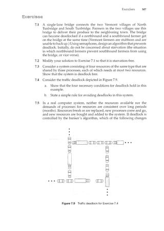
![310 Chapter 7
7.13 Consider the deadlock situation that can occur in the dining-
philosophers problem when the philosophers obtain the chopsticks one
at a time. Discuss how the four necessary conditions for deadlock hold
in this setting. Discuss how deadlocks could be avoided by eliminating
any one of the four necessary conditions.
7.14 What is the optimistic assumption made in the deadlock-detection
algorithm? How can this assumption be violated?
7.15 Consider the version of the dining-philosophers problem in which the
chopsticks are placed at the center of the table and any two of them
can be used by a philosopher. Assume that requests for chopsticks are
made one at a time. Describe a simple rule for determining whether a
particular request can be satisfied without causing deadlock given the
current allocation of chopsticks to philosophers.
7.16 Is it possible to have a deadlock involving only a single process? Explain
your answer.
7.17 Consider again the setting in the preceding question. Assume now that
each philosopher requires three chopsticks to eat. Resource requests are
still issued one at a time. Describe some simple rules for determining
whether a particular request can be satisfied without causing deadlock
given the current allocation of chopsticks to philosophers.
7.18 In Section 7.4.4, we describe a situation in which we prevent deadlock
by ensuring that all locks are acquired in a certain order. However,
we also point out that deadlock is possible in this situation if two
threads simultaneously invoke the transaction() function. Fix the
transaction() function to prevent deadlocks.
7.19 Write a multithreaded program that implements the banker's algorithm
discussed in Section 7.5.3. Create n threads that request and release
resources from the bank. The banker will grant the request only if it
leaves the system in a safe state. You may write this program using
either Pthreads or Win32 threads. It is important that shared data be safe
from concurrent access. To ensure safe access to shared data, you can
use mutex locks, which are available in both the Pthreads and Win32
APis. The use of mutex locks in both of these libraries is described in the
project entitled "Producer-Consumer Problem" at the end of Chapter 6.
Dijkstra [1965a] was one of the first and most influential contributors in the
deadlock area. Holt [1972] was the first person to formalize the notion of
deadlocks in terms of an allocation-graph model similar to the one presented
in this chapter. Starvation was also covered by Holt [1972]. Hyman [1985]
provided the deadlock example from the Kansas legislature. A recent study of
deadlock handling is provided in Levine [2003].](https://image.slidesharecdn.com/elecnwintjql7eggtsqw-operating-system-concepts-8th-editiona4-230117160154-4fa44b38/85/Operating_System_Concepts_8th_EditionA4-pdf-324-320.jpg)
![311
The various prevention algorithms were suggested by Havender [1968],
who devised the resource-ordering scheme for the IBM OS/360 systen'l.
The banker's algorithm for avoiding deadlocks was developed for a single
resource type by Dijkstra [1965a] and was extended to multiple resource types
by Habermam'l [1969]. Exercises 7.3 and 7.11 are from Holt [1971].
The deadlock-detection algorithm for multiple instances of a resource type,
which is described in Section 7.6.2, was presented by Coffman et al. [1971].
Bach [1987] describes how many of the algorithms in the traditional UNIX
kernel handle deadlock. Solutions to deadlock problems in networks are
discussed in works such as Culler et al. [1998] and Rodeheffer and Schroeder
[1991].
The witness lock-order verifier is presented in Baldwin [2002].](https://image.slidesharecdn.com/elecnwintjql7eggtsqw-operating-system-concepts-8th-editiona4-230117160154-4fa44b38/85/Operating_System_Concepts_8th_EditionA4-pdf-325-320.jpg)


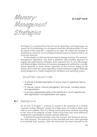
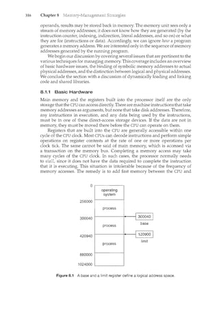
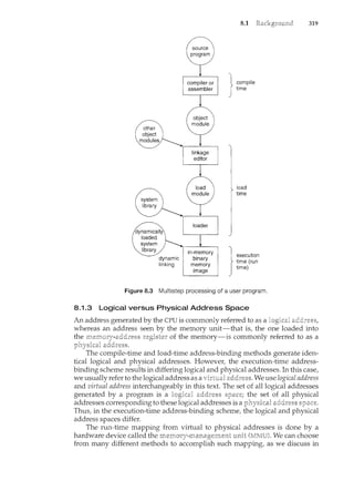
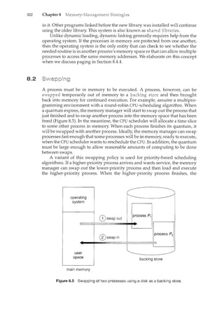
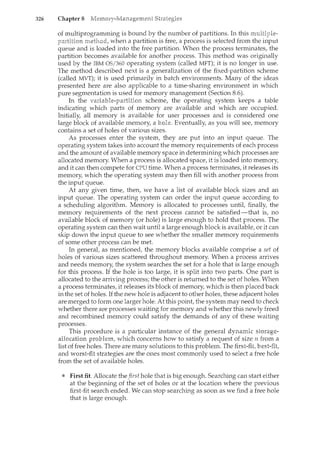
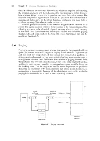
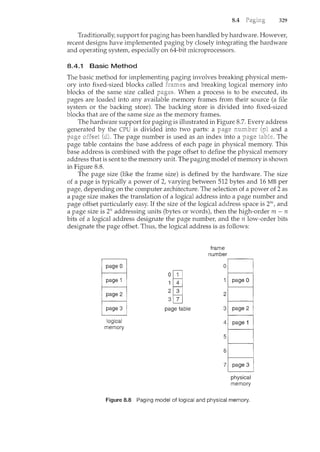
![330 Chapter 8
page number page offset
d
m -n n
where p is an index into the page table and d is the displacement within the
page.
As a concrete (although minuscule) example, consider the memory in
Figure 8.9. Here, in the logical address, n= 2 and m = 4. Using a page size
of 4 bytes and a physical memory of 32 bytes (8 pages), we show how the
user's view of memory can be mapped into physical memory. Logical address
0 is page 0, offset 0. Indexing into the page table, we find that page 0 is in frame
5. Thus, logical address 0 maps to physical address 20 [= (5 x 4) + 0]. Logical
address 3 (page 0, offset 3) maps to physical address 23 [= (5 x 4) + 3]. Logical
address 4 is page 1, offset 0; according to the page table, page 1 is mapped to
frame 6. Thus, logical address 4 maps to physical address 24 [= (6 x 4) + O].
Logical address 13 maps to physical address 9.
You may have noticed that paging itself is a form of dynamic relocation.
Every logical address is bound by the paging hardware to some physical
address. Using paging is similar to using a table ofbase (or relocation) registers,
one for each frame of memory.
~m6
2 1
3 2
page table
logical memory
physical memory
Figure 8.9 Paging example for a 32-byte memory with 4-byte pages.](https://image.slidesharecdn.com/elecnwintjql7eggtsqw-operating-system-concepts-8th-editiona4-230117160154-4fa44b38/85/Operating_System_Concepts_8th_EditionA4-pdf-344-320.jpg)
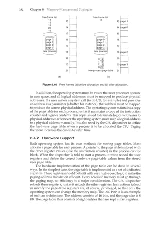
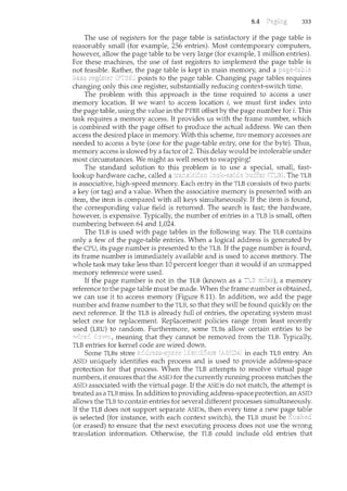
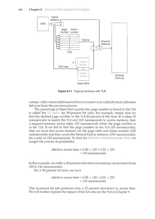
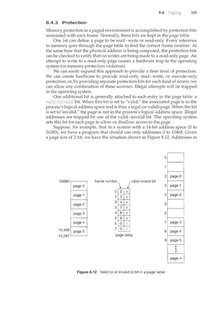
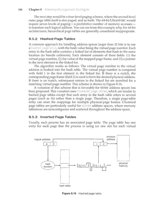
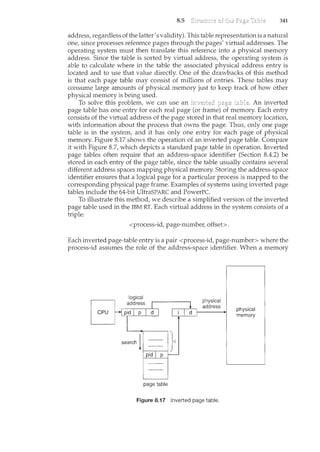
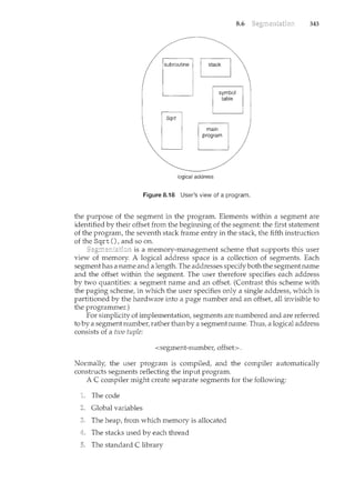
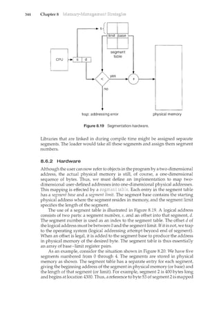
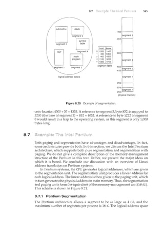
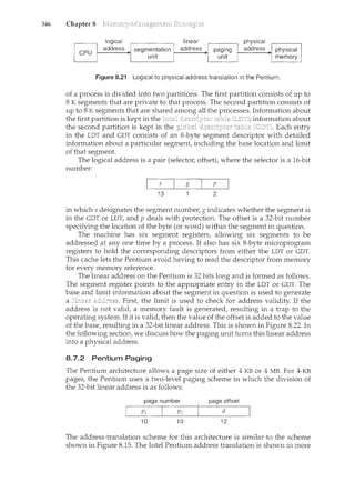
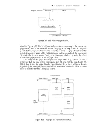
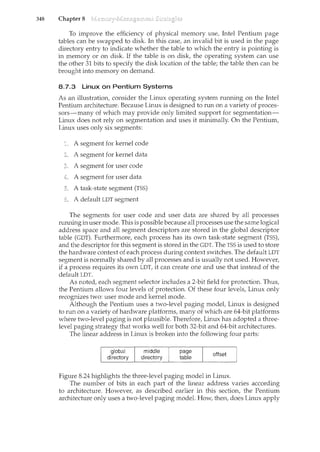
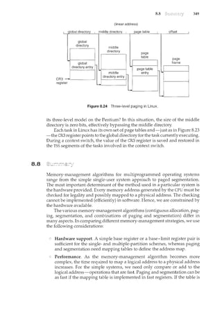
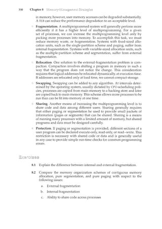

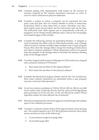
![354 Chapter 8
8.23 Sharing segments among processes without requiring that they have the
same segment number is possible in a dynamically linked segmentation
system.
a. Define a system that allows static linking and sharing of segments
without requiring that the segment numbers be the same.
b. Describe a paging scheme that allows pages to be shared without
requiring that the page numbers be the same.
8.24 Assume that a system has a 32-bit virtual address with a 4-KB page size.
Write a C program that is passed a virtual address (in decincal) on the
command line and have it output the page number and offset for the
given address. As an example, your program would run as follows:
./a.out 19986
Your program would output:
The address 19986 contains:
page number = 4
offset = 3602
Writing this program will require using the appropriate data type to
store 32 bits. We encourage you to use unsigned data types as well.
Dynamic storage allocation was discussed by Knuth [1973] (Section 2.5), who
found through simulation results that first fit is generally superior to best fit.
Knuth [1973] also discussed the 50-percent rule.
The concept of paging can be credited to the designers of the Atlas system,
which has been described by Kilburn et al. [1961] and by Howarth et al.
[1961]. The concept of segmentation was first discussed by Dennis [1965].
Paged segmentation was first supported in the GE 645, on which MULTICS was
originally implemented (Organick [1972] and Daley and Dennis [1967]).
Inverted page tables are discussed in an article about the IBM RT storage
manager by Chang and Mergen [1988].
Address translation in software is covered in Jacob and Mudge [1997].
Hennessy and Patterson [2002] explains the hardware aspects of TLBs,
caches, and MMUs. Talluri et al. [1995] discusses page tables for 64-bit address
spaces. Alternative approaches to enforcing memory protection are proposed
and studied in Wahbe et al. [1993a], Chase et al. [1994], Bershad et al. [1995],
and Thorn [1997]. Dougan et al. [1999] and Jacob and Mudge [2001] discuss](https://image.slidesharecdn.com/elecnwintjql7eggtsqw-operating-system-concepts-8th-editiona4-230117160154-4fa44b38/85/Operating_System_Concepts_8th_EditionA4-pdf-368-320.jpg)
![355
tedmiques for managing the TLB. Fang et al. [2001] evaluate support for large
pages.
Tanenbaum [2001] discusses Intel80386 paging. Memory management for
several architectures-such as the Pentiunl II, PowerPC, and UltraSPARC-
are described by Jacob and Mudge [1998a]. Segmentation on Lim1X systems is
presented in Bovet and Cesati [2002].](https://image.slidesharecdn.com/elecnwintjql7eggtsqw-operating-system-concepts-8th-editiona4-230117160154-4fa44b38/85/Operating_System_Concepts_8th_EditionA4-pdf-369-320.jpg)

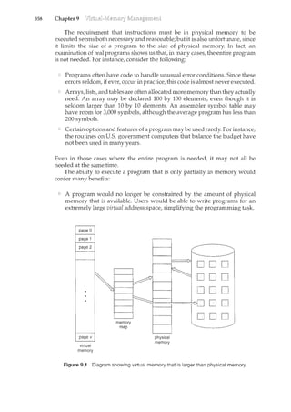
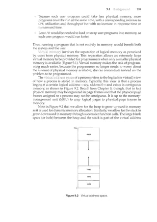
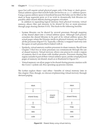
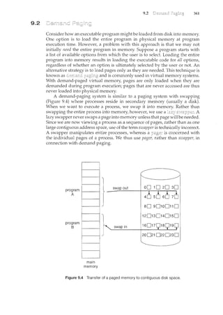
![362 Chapter 9
9.2.1 Basic Concepts
When a process is to be swapped in, the pager guesses which pages will be
used before the process is swapped out again. Instead of swapping in a whole
process, the pager brings only those pages into memory. Thus, it avoids reading
into memory pages that will not be used anyway, decreasing the swap time
and the amount of physical memory needed.
With this scheme, we need some form of hardware support to distinguish
between the pages that are in memory and the pages that are on the disk.
The valid-invalid bit scheme described in Section 8.4.3 can be used for this
purpose. This time, however, when this bit is set to "valid/' the associated page
is both legal and in n1.emory. If the bit is set to "invalid/' the page either is not
valid (that is, not in the logical address space of the process) or is valid but
is currently on the disk. The page-table entry for a page that is brought into
memory is set as usuat but the page-table entry for a page that is not currently
in memory is either simply marked invalid or contains the address of the page
on disk. This situation is depicted in Figure 9.5.
Notice that marking a page invalid will have no effect if the process never
attempts to access that page. Hence, if we guess right and page in all and only
those pages that are actually needed, the process will run exactly as though we
had brought in all pages. While the process executes and accesses pages that
are execution proceeds normally.
0
2
3
4
5
6
7
valid-invalid
frame bit
'. I
0 4 v
logical
memory
physical memory
DOD
D
[1J
[.@JtB]
ODD
Figure 9.5 Page table when some pages are not in main memory.](https://image.slidesharecdn.com/elecnwintjql7eggtsqw-operating-system-concepts-8th-editiona4-230117160154-4fa44b38/85/Operating_System_Concepts_8th_EditionA4-pdf-376-320.jpg)
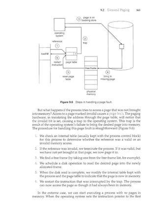
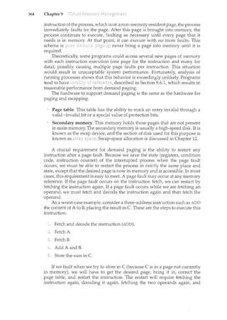
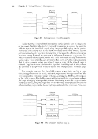
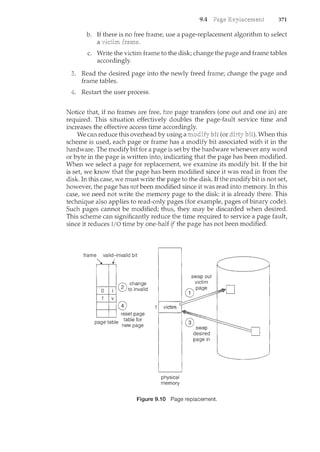
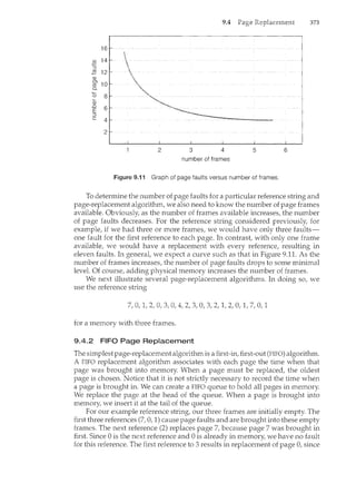
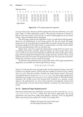
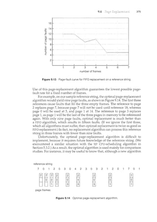
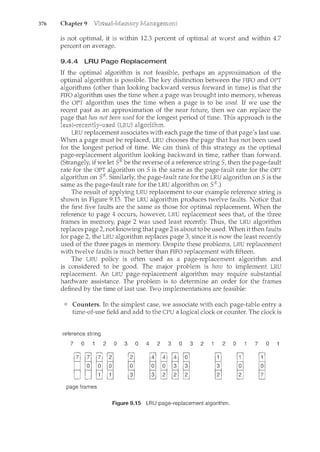
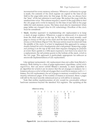
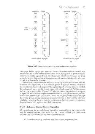
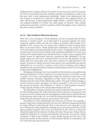
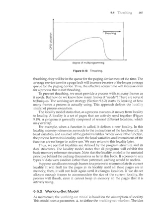
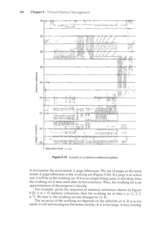
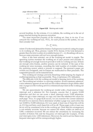
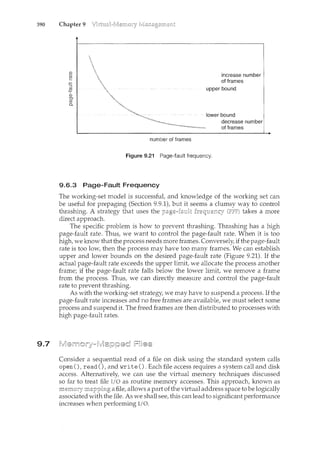
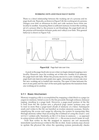
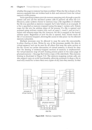
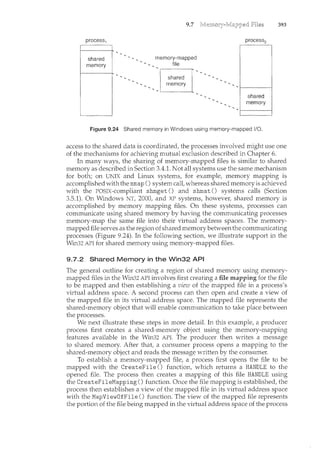
![394 Chapter 9
#include <windows.h>
#include <stdio.h>
int main(int argc, char *argv[])
{
}
HANDLE hFile, hMapFile;
LPVOID lpMapAddress;
hFile = CreateFile("temp.txt", //file name
GENERICJREAD I GENERIC_WRITE, // read/write access
0, II no sharing of the file
NULL, //default security
OPEN_ALWAYS, //open new or existing file
FILE_ATTRIBUTE_NORMAL, //routine file attributes
NULL); //no file template
hMapFile = CreateFileMapping(hFile, //file handle
NULL, //default security
PAGEJREADWRITE, //read/write access to mapped pages
0, II map entire file
0,
TEXT("SharedObject")); //named shared memory object
lpMapAddress = MapViewDfFile(hMapFile, //mapped object handle
FILEJMAP_ALL_ACCESS, //read/write access
0, II mapped view of entire file
0,
0);
II write to shared memory
sprintf(lpMapAddress,"Shared memory message");
UnmapViewOfFile(lpMapAddress);
CloseHandle(hFile);
CloseHandle(hMapFile);
Figure 9.25 Producer writing to shared memory using the Win32 API.
-the entire file or only a portion of it may be mapped. We illustrate this
sequence in the program shown in Figure 9.25. (We eliminate much of the error
checking for code brevity.)
The call to CreateFileMapping() creates a named shared-memory object
called SharedObj ect. The consumer process will communicate using this
shared-memory segment by creating a mapping to the same named object.
The producer then creates a view of the memory-mapped file in its virtual
address space. By passing the last three parameters the value 0, it indicates
that the mapped view is the entire file. It could instead have passed values
specifying an offset and size, thus creating a view containing only a subsection
of the file. (It is important to note that the entire mapping may not be loaded](https://image.slidesharecdn.com/elecnwintjql7eggtsqw-operating-system-concepts-8th-editiona4-230117160154-4fa44b38/85/Operating_System_Concepts_8th_EditionA4-pdf-408-320.jpg)
![#include <windows.h>
#include <stdio.h>
int main(int argc, char *argv[])
{
HANDLE hMapFile;
LPVOID lpMapAddress;
9.7 395
hMapFile = OpenFileMapping(FILE_MAP_ALL_ACCESS, // R/W access
FALSE, //no inheritance
}
TEXT("SharedObject")); //name of mapped file object
lpMapAddress = MapViewOfFile(hMapFile, //mapped object handle
FILEJMAP_ALL_ACCESS, //read/write access
0, II mapped view of entire file
0,
0);
II read from shared memory
printf("Read message %s", lpMapAddress);
UnmapViewOfFile(lpMapAddress);
CloseHandle(hMapFile);
Figure 9.26 Consumer reading from shared memory using the Win32 API.
into memory when the mapping is established. Rather, the mapped file may be
demand-paged, thus bringing pages into memory only as they are accessed.)
The MapViewOfFile () fm1ction returns a pointer to the shared-memory object;
any accesses to this memory location are thus accesses to the memory-mapped
file. In this ii1stance, the producer process writes the message "Shared memory
message" to shared memory.
A program illustrating how the consumer process establishes a view of
the named shared-memory object is shown in Figure 9.26. This program is
somewhat simpler than the one shown in Figure 9.25, as all that is necessary
is for the process to create a mapping to the existii1g named shared-memory
object. The consumer process must also create a view of the mapped file, just
as the producer process did ii1 the program in Figure 9.25. The consumer then
reads from shared memory the message "Shared memory message" thatwas
written by the producer process.
Finally, both processes remove the view of the mapped file with a call to
UnmapViewOfFile (). We provide a programming exercise at the end of this
chapter using shared memory with memory mapping in the Win32 API.
9.7.3 Memory-Mapped i/0
In the case of I/0, as mentioned in Section 1.2.1, each I/0 controller includes
registers to hold commands and the data being transferred. Usually, special I/0
instructions allow data transfers between these registers and system memory.](https://image.slidesharecdn.com/elecnwintjql7eggtsqw-operating-system-concepts-8th-editiona4-230117160154-4fa44b38/85/Operating_System_Concepts_8th_EditionA4-pdf-409-320.jpg)
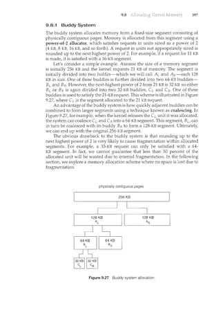
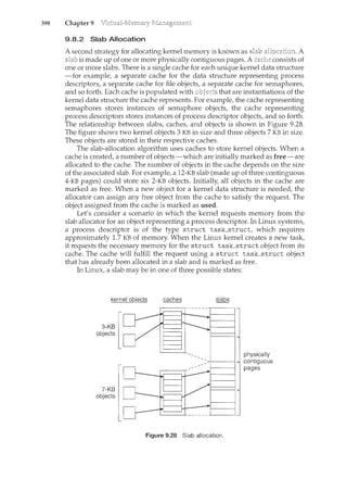
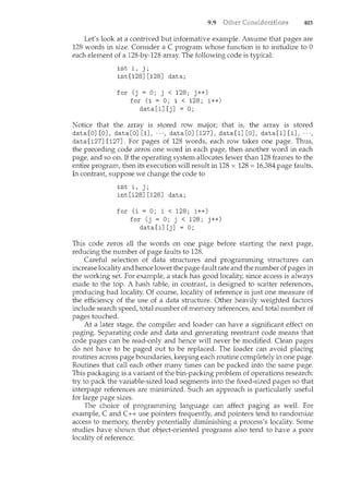
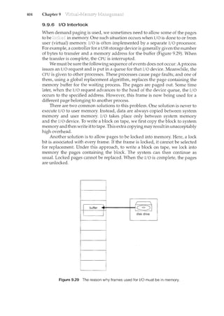
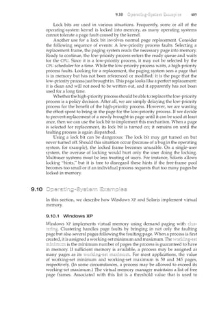
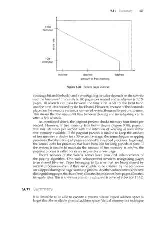
![413
9.15 What is the copy-on-write feature, and under what circumstances is it
beneficial to use this feature? What hardware support is required to
implement this feature?
9.16 Consider the two-dimensional array A:
int A[] [] = new int [100] [100] ;
where A[OJ [OJ is at location 200 in a paged memory system with pages
of size 200. A small process that manipulates the matrix resides in page
0 (locations 0 to 199). Thus, every instruction fetch will be from page 0.
For three page frames, how many page faults are generated by
the following array-initialization loops, using LRU replacement and
assuming that page frame 1 contains the process and the other two
are initially empty?
a. for (int j = 0; j < 100; j++)
for (int i = 0; i < 100; i++)
A[i] [j] = 0;
b. for (int i = 0; i < 100; i++)
for (int j = 0; j < 100; j++)
A[i] [j] = 0;
9.17 Discuss situations in which the least frequently used page-replacement
algorithm generates fewer page faults than the least recently used
page-replacement algorithm. Also discuss under what circumstances
the opposite holds.
9.18 What is the cause of thrashing? How does the system detect thrashing?
Once it detects thrashing, what can the system do to eliminate this
problem?
9.19 Assume that you are monitoring the rate at which the pointer in the
clock algorithm (which indicates the candidate page for replacement)
moves. What can you say about the system if you notice the following
behavior:
a. Pointer is moving fast.
b. Pointer is moving slow.
9.20 The VAX/VMS system uses a FIFO replacement algorithm for resident
pages and a free-frame pool of recently used pages. Assume that the
free-frame pool is managed using the least recently used replacement
policy. Answer the following questions:
a. If a page fault occurs and if the page does not exist in the free-frame
pool, how is free space generated for the newly requested page?](https://image.slidesharecdn.com/elecnwintjql7eggtsqw-operating-system-concepts-8th-editiona4-230117160154-4fa44b38/85/Operating_System_Concepts_8th_EditionA4-pdf-427-320.jpg)
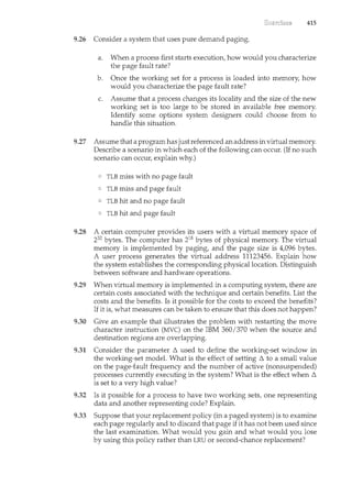
![416 Chapter 9
9.34 Write a program that implements the FIFO and LRU page-replacement
algorithms presented in this chapter. First, generate a random page-
reference string where page numbers range from 0 to 9. Apply the
random page-reference string to each algorithm, and record the number
of page faults incurred by each algorithm. Implement the replacement
algorithms so that the number of page frames can vary from 1 to 7.
Assume that demand paging is used.
9.35 The Catalan numbers are an integer sequence C11 that appear in tree-
enumeration problems. The first Catalan numbers for n = 1, 2, 3, ... are
1, 2, 5, 14, 42, 132, .... A formula generating C11 is
1 (2n) (2n)!
ell = (n + 1) --;; = (n + 1)!n!
Design two programs that communicate with shared memory using
the Win32 API as outlined in Section 9.7.2. The producer process will
generate the Catalan sequence and write it to a shared memory object.
The consumer process will then read and output the sequence from
shared memory.
In this instance, the producer process will be passed an integer
parameter on the command line specifying how many Catalan numbers
to produce (for example, providing 5 on the command line means the
producer process will generate the first five Catalan numbers).
Demand paging was first used iil the Atlas system, implemented on the
Manchester University MUSE computer around 1960 (Kilburn et al. [1961]).
Another early demand-paging system was MULTICS, implemented on the GE
645 system (Organick [1972]).
Belady et al. [1969] were the first researchers to observe that the FIFO
replacement strategy may produce the anomaly that bears Belady's name.
Mattson et al. [1970] demonstrated that stack algorithms are not subject to
Belady's anomaly.
The optimal replacement algorithm was presented by Belady [1966] and
was proved to be optimalby Mattson et al. [1970]. Belady's optimal algorithm is
for a fixed allocation; Prieve and Fabry [1976] presented an optimal algorithm
for situations in which the allocation can vary.
The enl"lanced clock algorithm was discussed by Carr and Hennessy [1981].
The working-set model was developed by Denning [1968]. Discussions
concerning the working-set model were presented by Denning [1980].
The scheme for monitoring the page-fault rate was developed by Wulf
[1969], who successfully applied this technique to the Burroughs BSSOO com-
puter system.
Wilson et al. [1995] presented several algoritluns for dynamic memory allo-
cation. Jolmstone and Wilson [1998] described various memory-fragmentation](https://image.slidesharecdn.com/elecnwintjql7eggtsqw-operating-system-concepts-8th-editiona4-230117160154-4fa44b38/85/Operating_System_Concepts_8th_EditionA4-pdf-430-320.jpg)
![417
issues. Buddy system memory allocators were described in Knowlton [1965L
Peterson and Norman [1977], and Purdom, Jr. and Stigler [1970]. Bonwick
[1994] discussed the slab allocator, and Bonwick and Adams [2001] extended
the discussion to multiple processors. Other memory-fitting algorithms can
be found in Stephenson [1983], Bays [1977], and Brent [1989]. A survey of
memory-allocation strategies can be found in Wilson et al. [1995].
Solomon and Russinovich [2000] and Russinovich and Solomon [2005]
described how Windows implements virtual memory. McDougall and Mauro
[2007] discussed virtual memory in Solaris. Virtual memory techniques in
Linux and BSD were described by Bovet and Cesati [2002] and McKusick
et al. [1996], respectively. Ganapathy and Schimmel [1998] and Navarro et al.
[2002] discussed operating system support for multiple page sizes. Ortiz [2001]
described virtual memory used in a real-time embedded operating system.
Jacob and Mudge [1998b] compared implementations of virtual memory in
the MIPS, PowerPC, and Pentium architectures. A companion article (Jacob and
Mudge [1998a]) described the hardware support necessary for implementation
of virtual memory in six different architectures, including the UltraSPARC.](https://image.slidesharecdn.com/elecnwintjql7eggtsqw-operating-system-concepts-8th-editiona4-230117160154-4fa44b38/85/Operating_System_Concepts_8th_EditionA4-pdf-431-320.jpg)


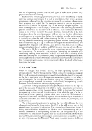
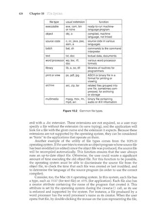
![10.2 431
beginning
current position
end
<];:::::,,,===, rewind~ read or write~
Figure 10.3 Sequential-access file.
10.2.1 Sequential Access
The simplest access method is . Information in the file is
processed in order, one record after the other. This mode of access is by far the
most common; for example, editors and compilers usually access files in this
fashion.
Reads and writes make up the bulk of the operations on a file. A read
operation-read next-reads the next portion of the file and automatically
advances a file pointer, which tracks the I/O location. Similarly, the write
operation-write next-appends to the end of the file and advances to the
end of the newly written material (the new end of file). Such a file can be reset
to the beginning; and on some systems, a program may be able to skip forward
or backward n records for some integer n-perhaps only for n = 1. Sequential
access, which is depicted in Figure 10.3, is based on a tape model of a file and
works as well on sequential-access devices as it does on random-access ones.
10.2.2 Direct Access
(or A file is made up of fixed-
length that allow programs to read and write records rapidly
in no particular order. The direct-access method is based on a disk model of
a file, since disks allow random access to any file block. For direct access, the
file is viewed as a numbered sequence of blocks or records. Thus, we may read
block 14, then read block 53, and then write block 7. There are no restrictions
on the order of reading or writing for a direct-access file.
Direct-access files are of great use for immediate access to large amounts
of information. Databases are often of this type. When a query concerning a
particular subject arrives, we compute which block contains the answer and
then read that block directly to provide the desired information.
As a simple example, on an airline-reservation system, we might store all
the information about a particular flight (for example, flight 713) in the block
identified by the flight number. Thus, the number of available seats for flight
713 is stored in block 713 of the reservation file. To store il1formation about a
larger set such as people, we might compute a hash function on the people's
names or search a small in-ncemory index to determine a block to read and
search.
For the direct-access method, the file operations must be modified to
include the block number as a parameter. Thus, we have read n, where n is
the block number, rather than read next, and ·write n rather than write next. An
alternative approach is to retain read next and write next, as with sequential](https://image.slidesharecdn.com/elecnwintjql7eggtsqw-operating-system-concepts-8th-editiona4-230117160154-4fa44b38/85/Operating_System_Concepts_8th_EditionA4-pdf-445-320.jpg)
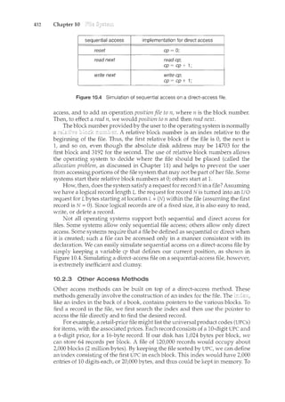
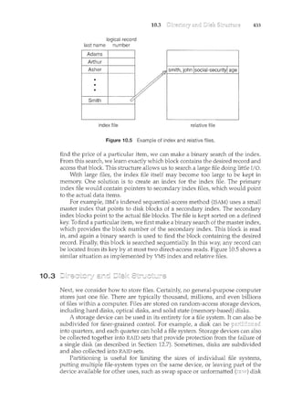
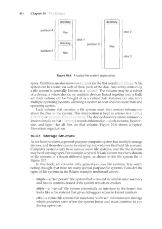
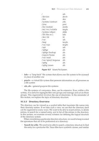
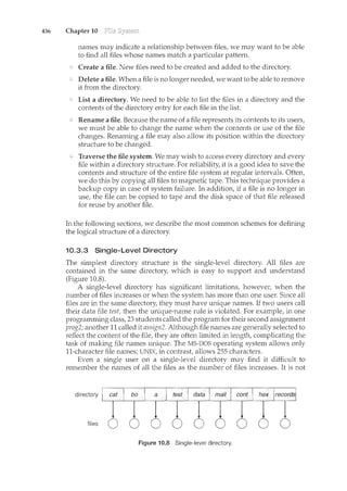
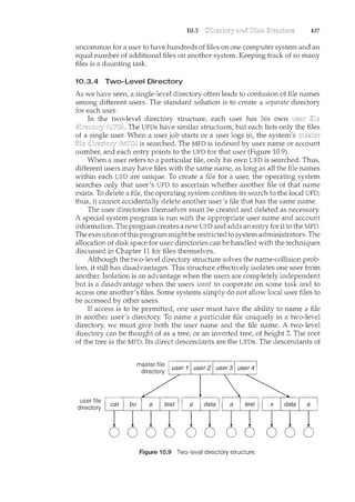
![438 Chapter 10
the UFDs are the files themselves. The files are the leaves of the tree. Specifying
a user name and a file name defines a path in the tree from the root (the MFD)
to a leaf (the specified file). Thus, a user name and a file name define a path
name. Every file in the system has a path name. To name a file uniquely, a user
must know the path name of the file desired.
For example, if user A wishes to access her own test file named test, she can
simply refer to test. To access the file named test of user B (with directory-entry
name userb), however, she might have to refer to /userb/test. Every system has
its own syntax for naming files in directories other than the user's own.
Additional syntax is needed to specify the volume of a file. For instance,
in MS-DOS a volume is specified by a letter followed by a colon. Thus, a file
specification mightbe C:userbfest. Some systems go even further and separate
the volume, directory name, and file name parts of the specification. For
instance, in VMS, the file login.com might be specified as: u:[sst.jdeck]login.com;l,
where u is the name of the volume, sst is the name of the directory, jdeck is the
name of the subdirectory, and 1 is the version number. Other systems simply
treat the volume name as part of the directory name. The first name given is
that of the volume, and the rest is the directory and file. For instance, /u/pbg/test
might specify volume u, directory pbg, and file test.
A special case of this situation occurs with the system files. Programs pro-
vided as part of the system-loaders, assemblers, compilers, utility routines,
libraries, and so on-are generally defined as files. When the appropriate
commands are given to the operating system, these files are read by the loader
and executed. Many command interpreters simply treat such a command as the
name of a file to load and execute. As the directory system is defined presently,
this file name would be searched for in the current UFD. One solution would
be to copy the system files into each UFD. However, copying all the system files
would waste an enormous amount of space. (If the system files require 5 MB,
then supporting 12 users would require 5 x 12 == 60 MB just for copies of the
system files.)
The standard solution is to complicate the search procedure slightly. A
special user directory is defined to contain the system files (for example, user
0). Whenever a file name is given to be loaded, the operating system first
searches the local UFD. If the file is found, it is used. Ifit is not found, the system
automatically searches the special user directory that contains the system files.
The sequence of directories searched when a file is named is called the
. The search path can be extended to contain an unlimited list of directories
to search when a command name is given. This method is the one most used
in UNIX and MS-DOS. Systems can also be designed so that each user has his
own search path.
10.3.5 Tree-Structured Directories
Once we have seen how to view a two-level directory as a two-level tree,
the natural generalization is to extend the directory structure to a tree of
arbitrary height (Figure 10.10). This generalization allows users to create their
own subdirectories and to organize their files accordingly. A tree is the most
common directory structure. The tree has a root directory, and every file in the
system has a unique path name.](https://image.slidesharecdn.com/elecnwintjql7eggtsqw-operating-system-concepts-8th-editiona4-230117160154-4fa44b38/85/Operating_System_Concepts_8th_EditionA4-pdf-452-320.jpg)
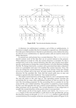
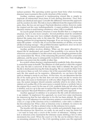
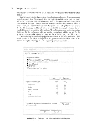
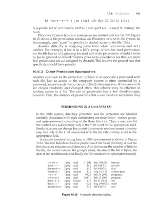

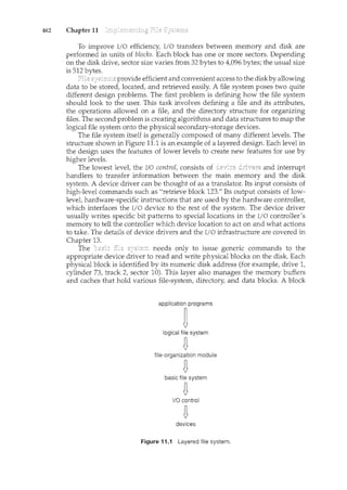
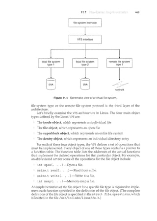
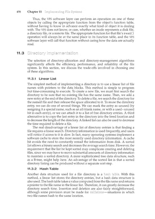
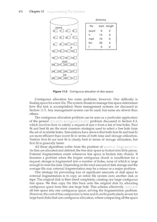
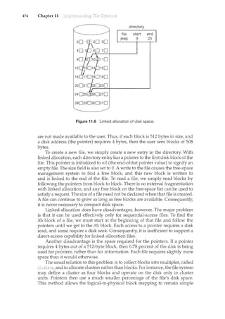
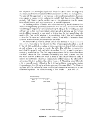
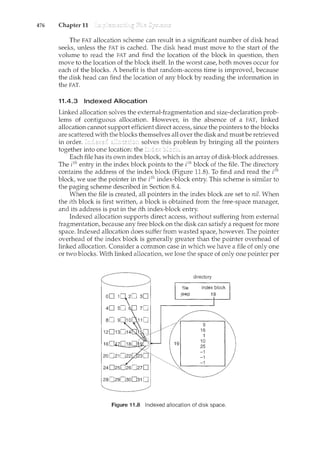
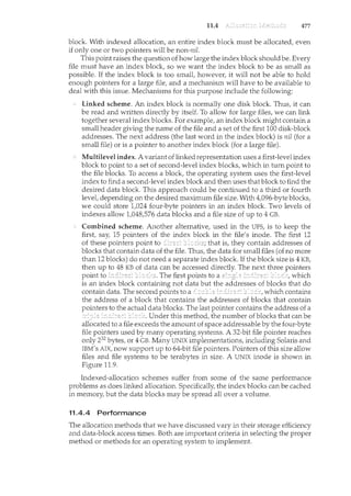
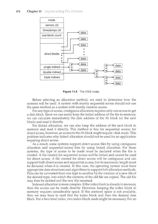
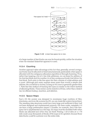
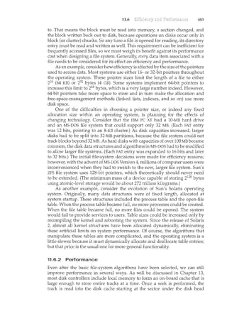
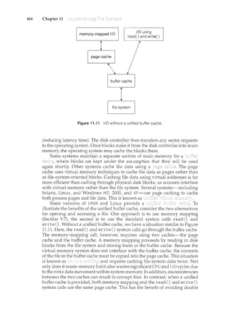
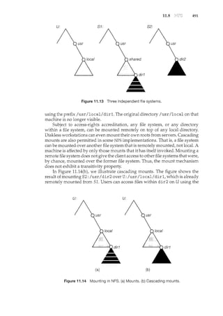
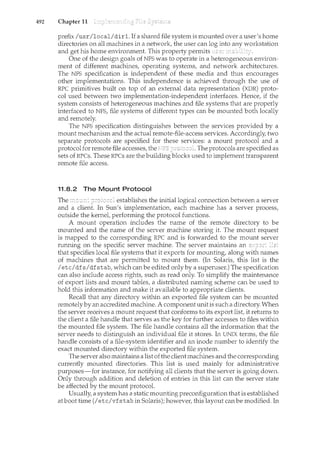
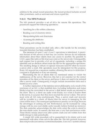
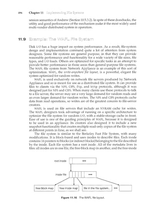
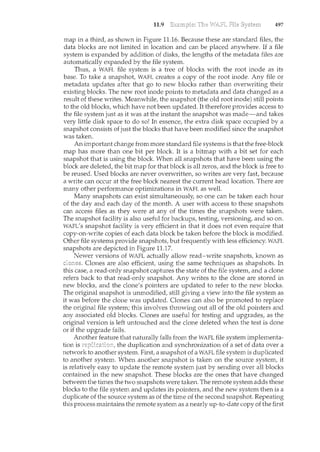
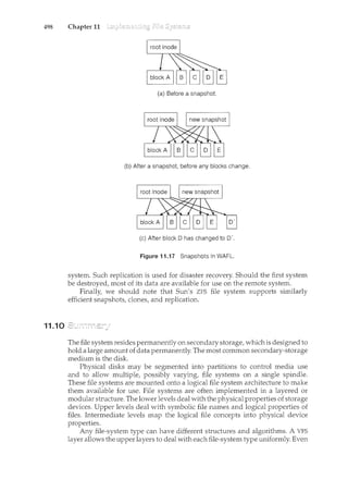

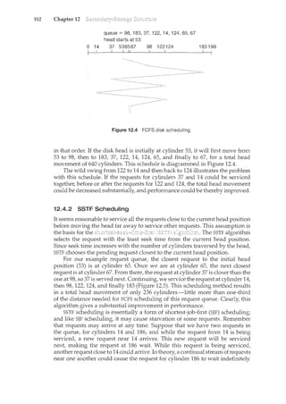
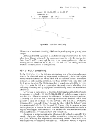
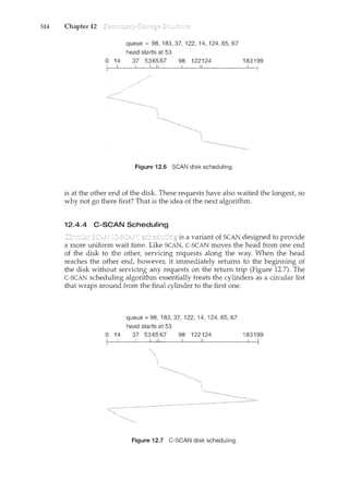
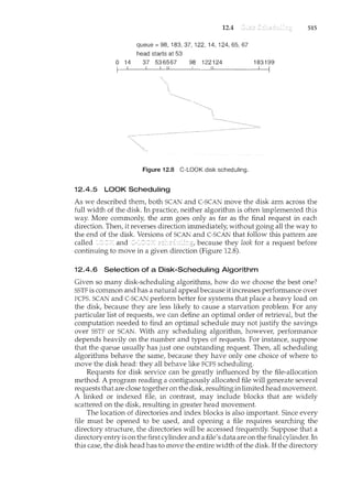
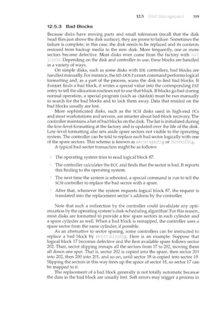
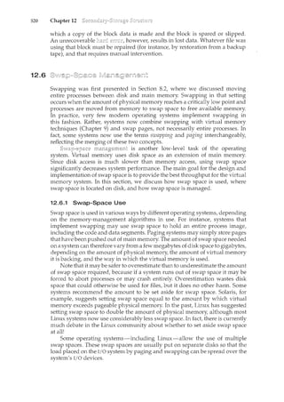
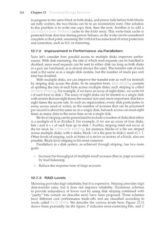
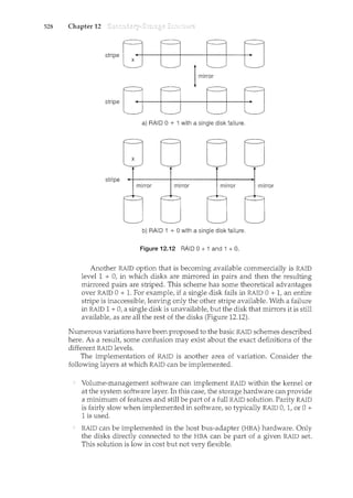
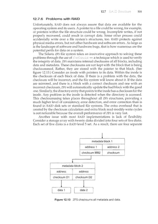
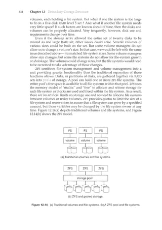
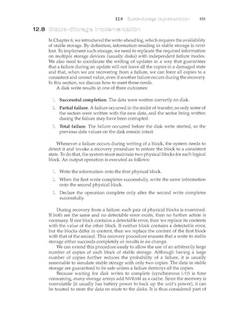
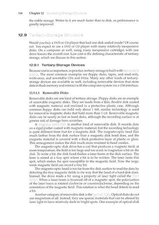
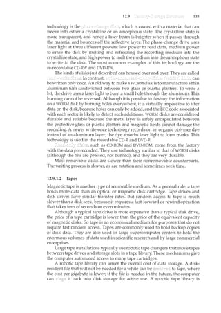
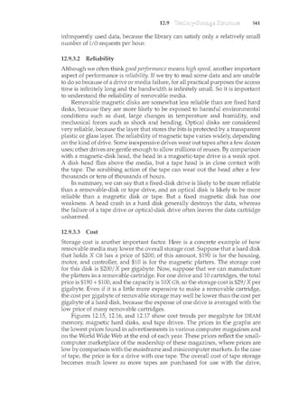
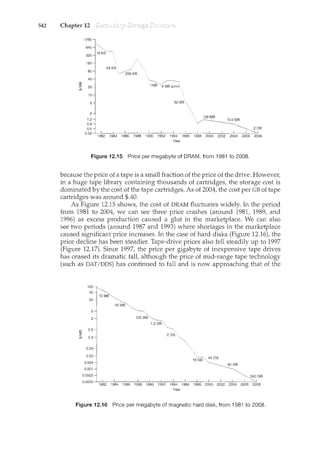
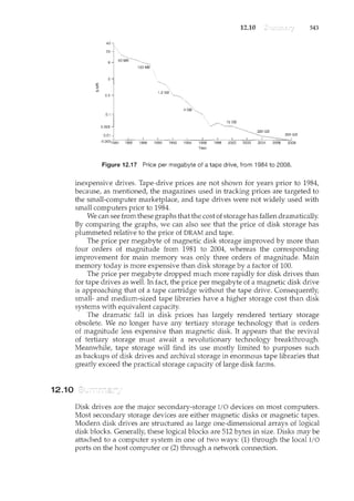
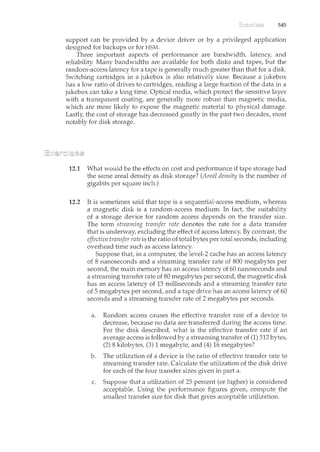
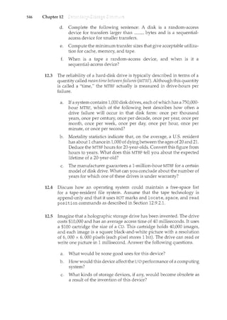
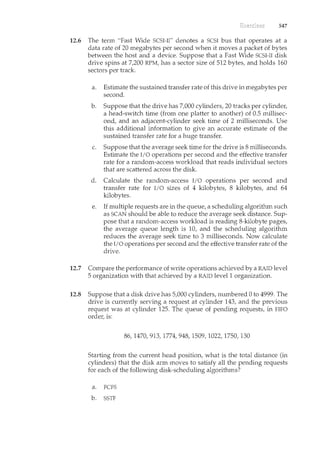

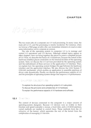
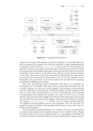
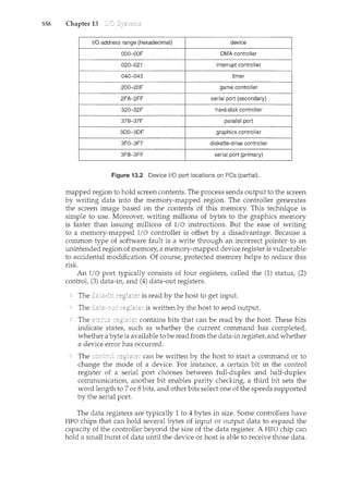
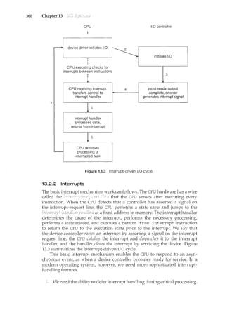
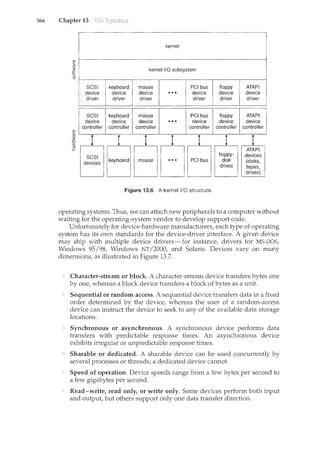
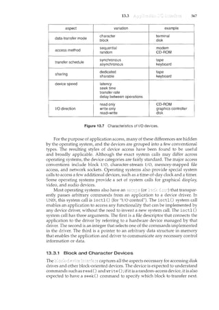
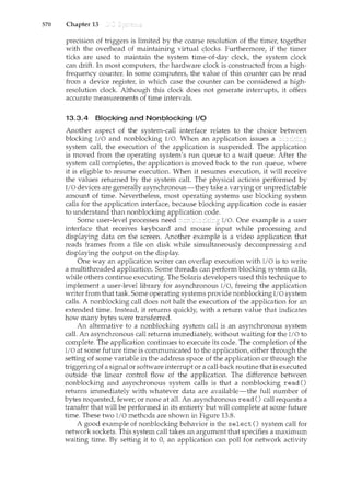
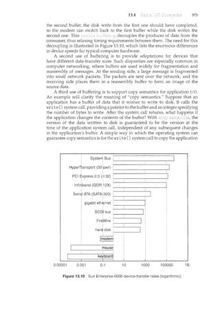
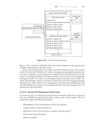
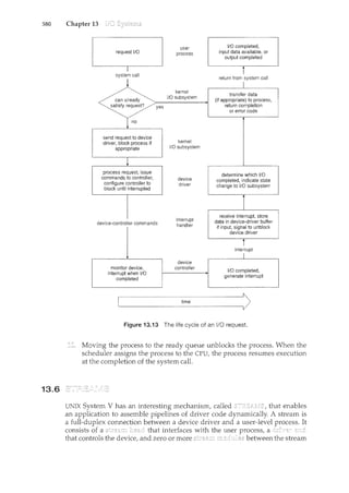
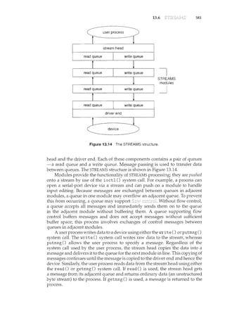
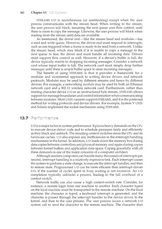
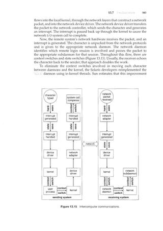
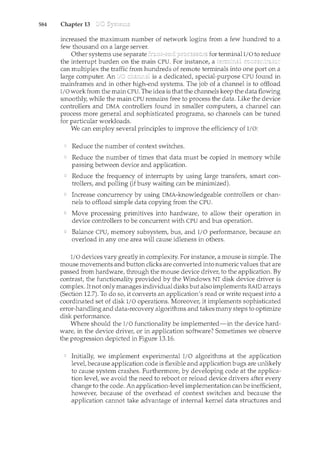
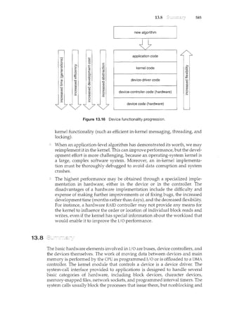


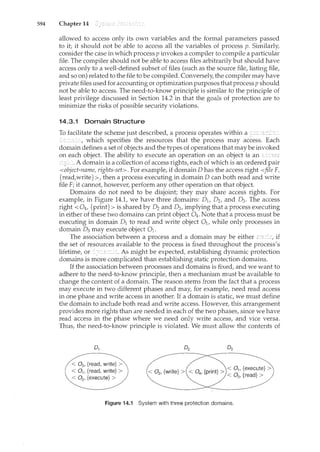
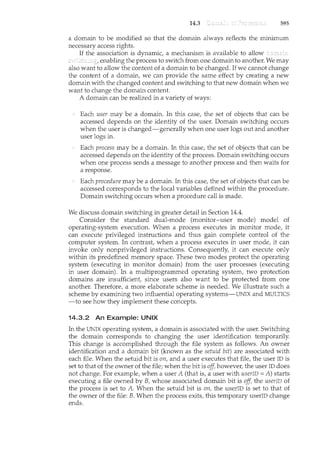
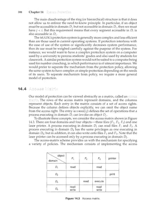
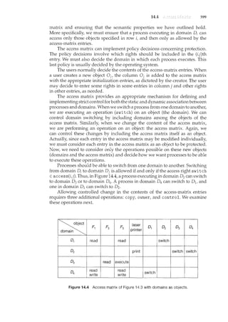
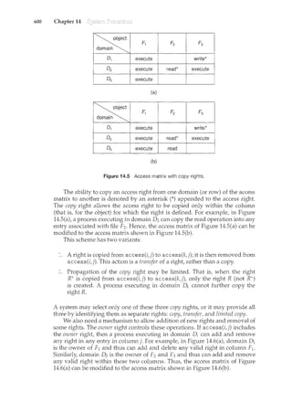
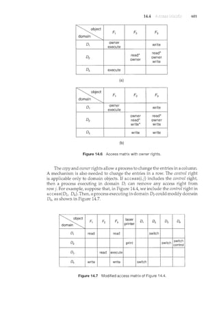
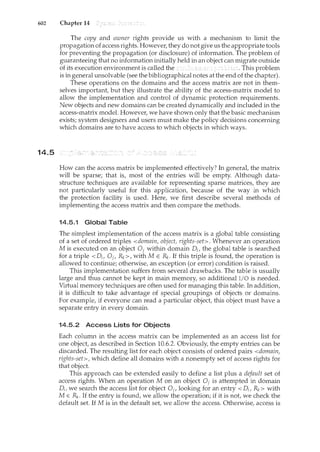
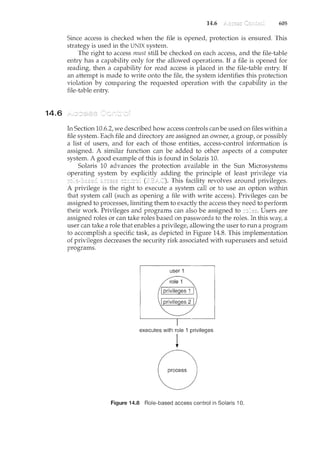
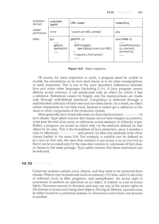
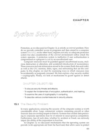
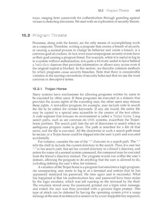
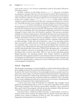
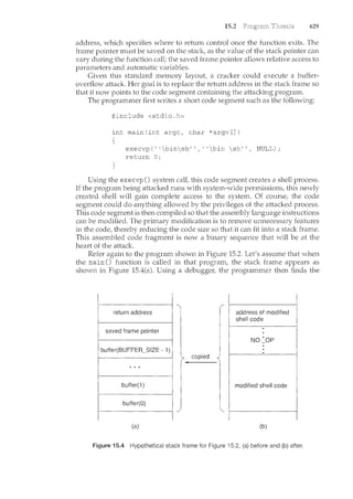
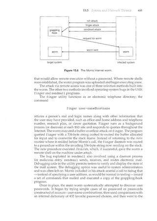
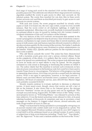
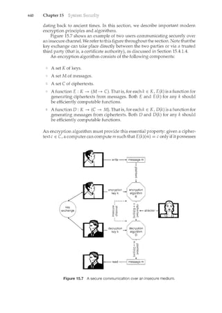
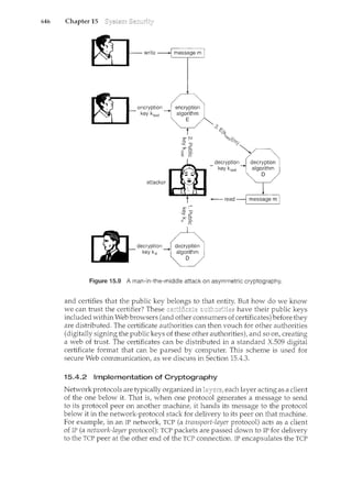
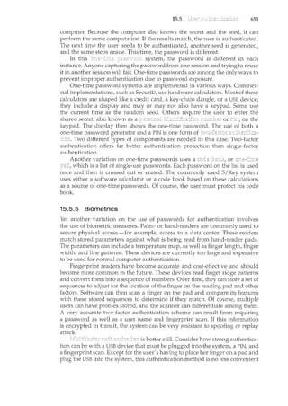
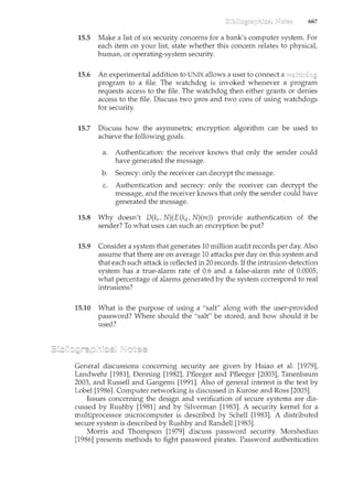

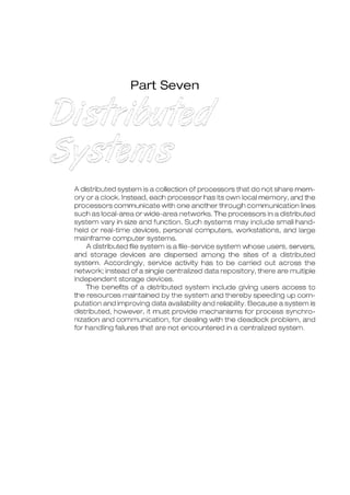

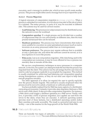
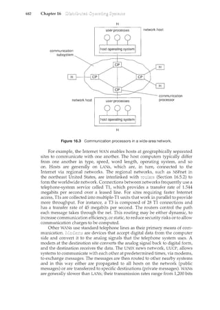
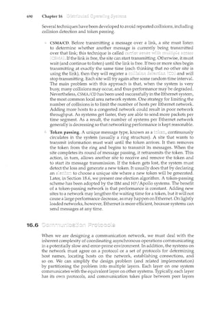
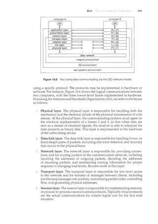
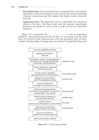
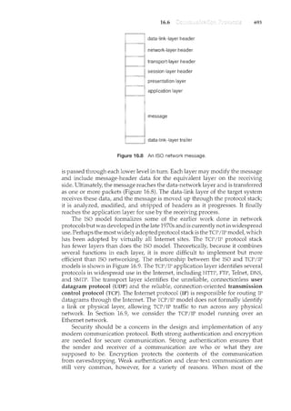
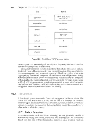
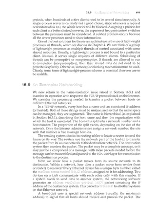
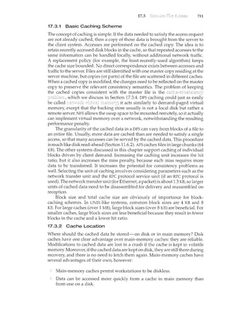

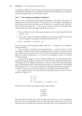
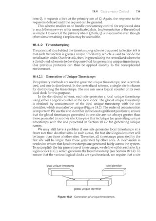
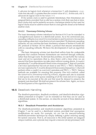
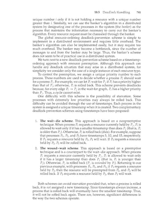
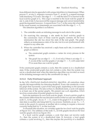


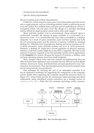
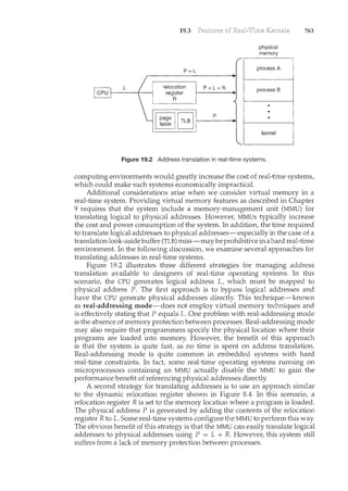
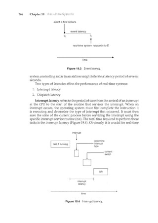
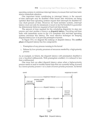
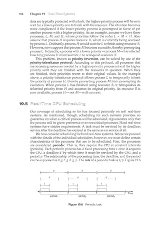
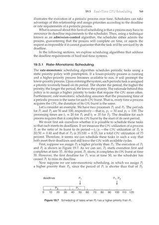
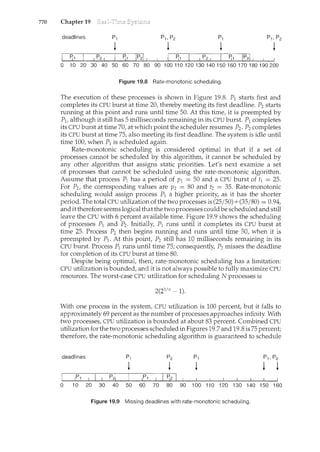
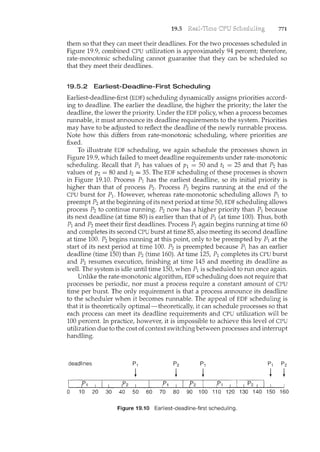
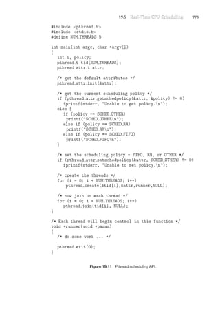
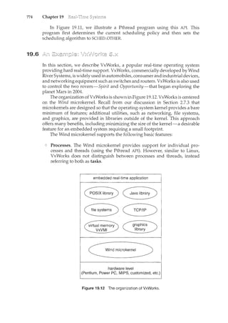

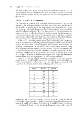
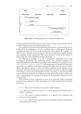
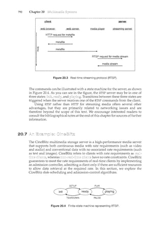
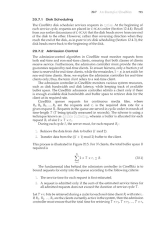
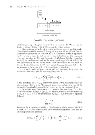


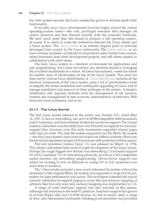
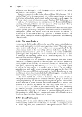
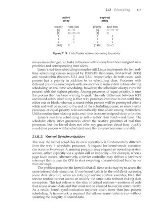
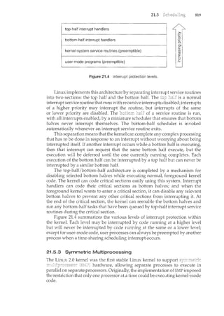
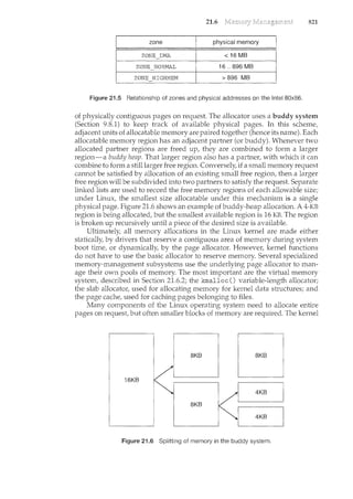
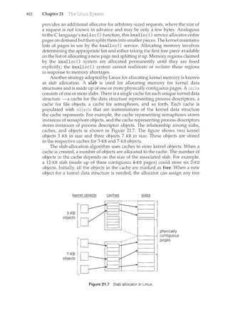
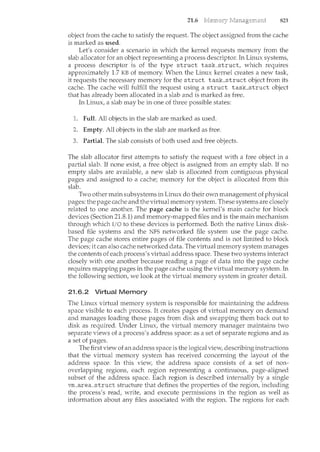
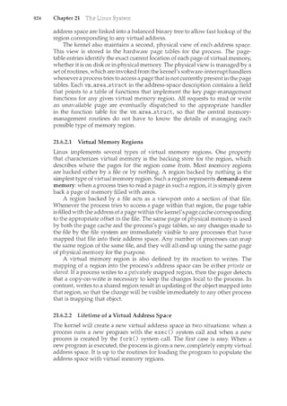
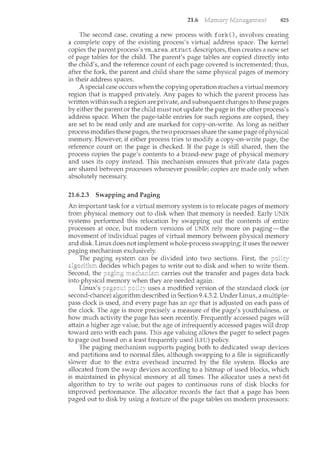
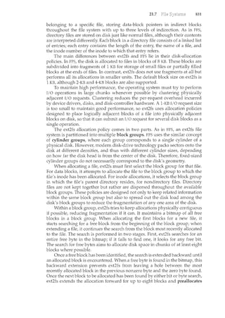
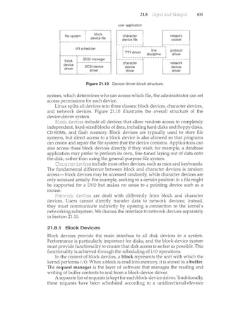
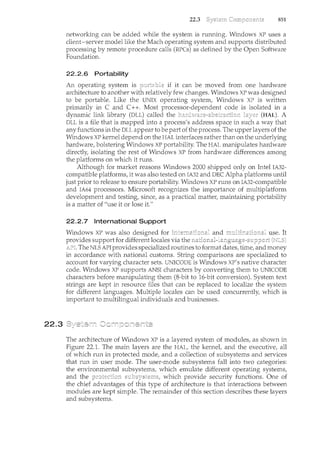
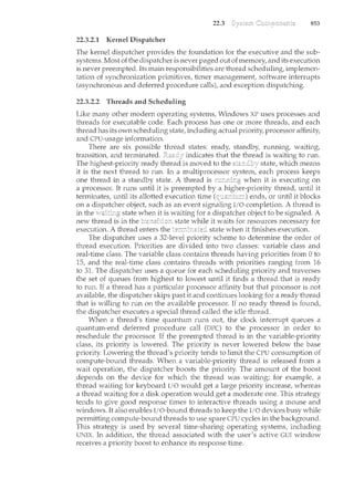
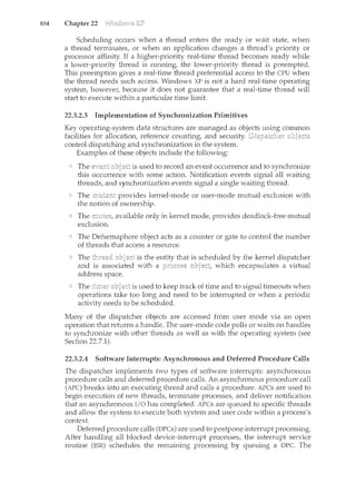
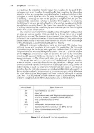
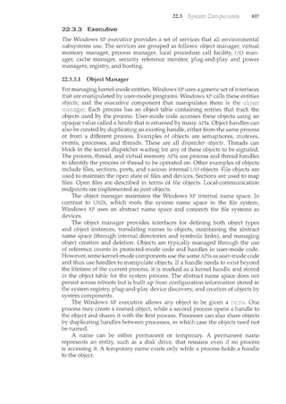
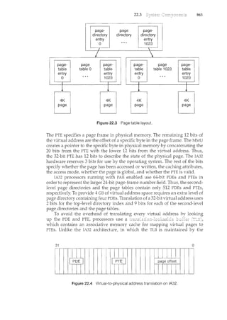
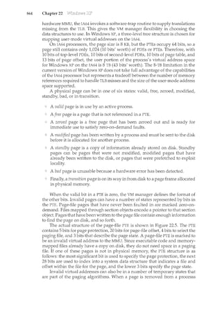
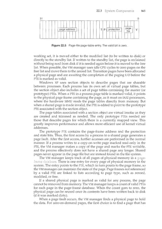
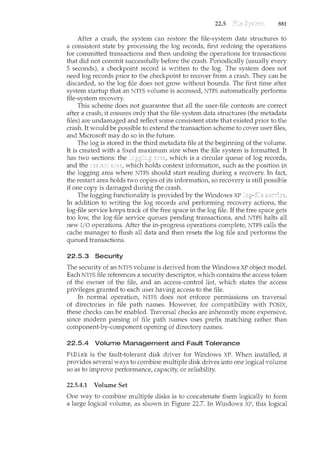
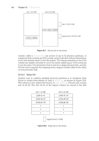
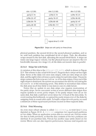
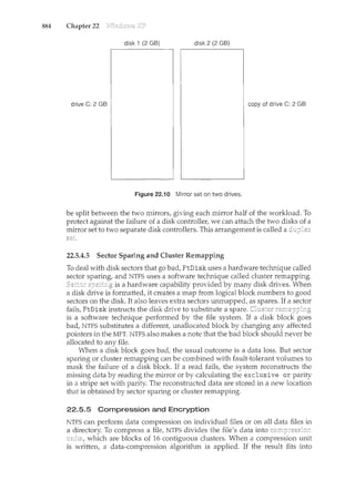
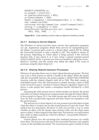
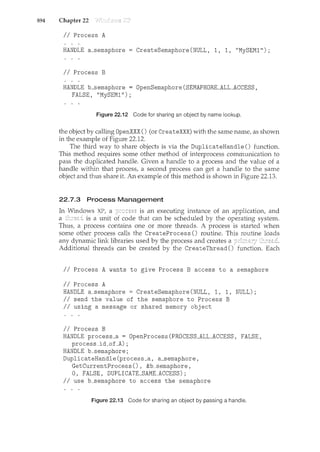
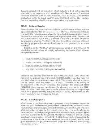

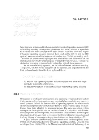
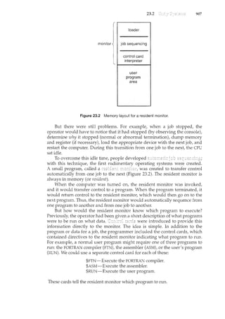
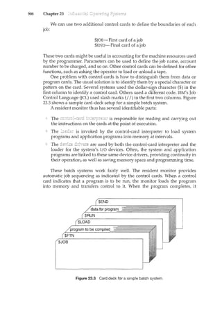
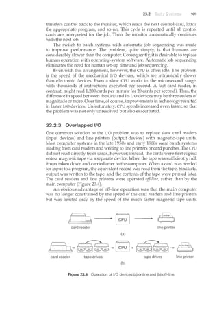
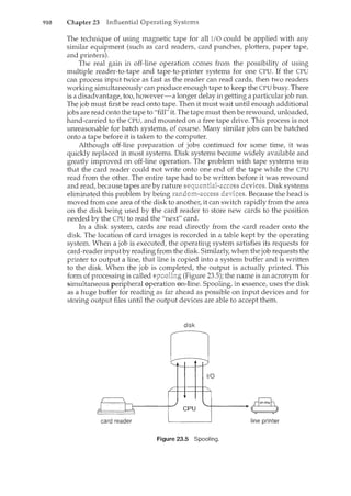

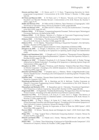
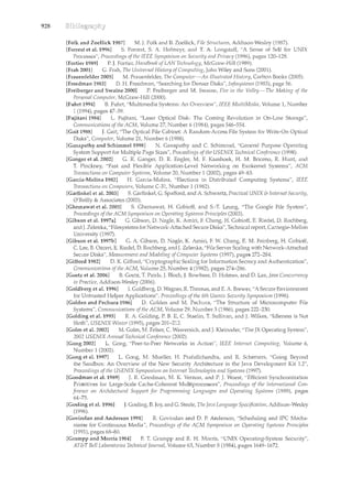
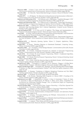
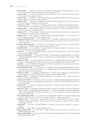
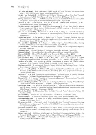
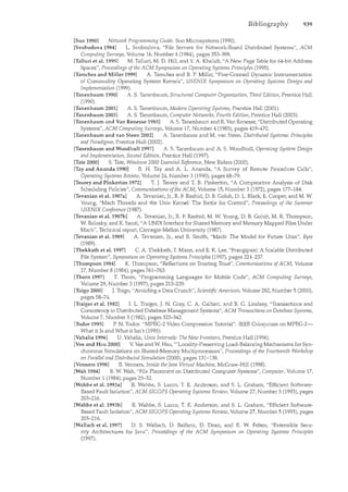
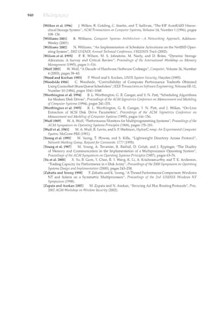

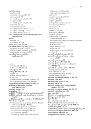
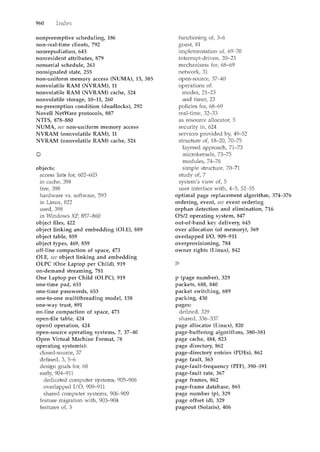
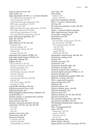
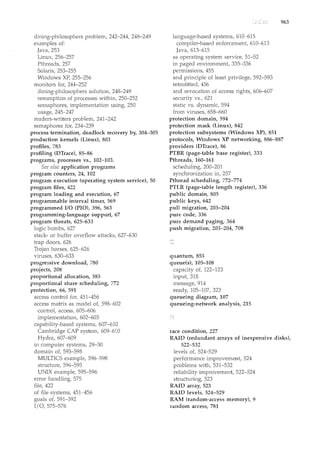
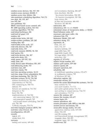
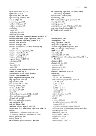


![ADBB_204_Operating_System_10_09_2024[1].pptx](https://cdn.slidesharecdn.com/ss_thumbnails/adbb204operatingsystem100920241-241122113715-620cd04a-thumbnail.jpg?width=640&height=640&fit=bounds)