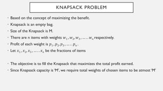
The document provides an introduction to greedy algorithms, explaining their characteristics such as the greedy choice property and optimal substructure, and emphasizes their application in optimization problems like the knapsack problem and Dijkstra's algorithm. It details various techniques and examples, including both fractional and 0/1 knapsack problems, and presents methods for finding minimum spanning trees through Prim's and Kruskal's algorithms. The key takeaway is that while greedy methods are simple and efficient, they may not always yield optimal solutions.

1. GREEDY ALGORITHMS
AOA Module 2

2. INTRODUCTION
• The greedy method is one of the strategies like Divide and conquer used to solve the
problems.
• The Greedy method is the simplest and straightforward approach. It is not an algorithm,
but it is a technique.
• Used for solving optimization problems.
• Decision is taken based on the currently available information.
• This technique is basically used to determine the feasible solution that may or may not
be optimal.
• The feasible solution is a subset that satisfies the given criteria.
• The optimal solution is the solution which is the best and the most favorable solution in
the subset.
• In the case of feasible, if more than one solution satisfies the given criteria then those
solutions will be considered as the feasible, whereas the optimal solution is the best
solution among all the solutions.

3. INTRODUCTION
General Characteristics
1. Greedy choice Property:
Globally optimal solution can be arrived at by making a locally optimal choice.
Greedy choices are made one after another, reducing each given problem instance to smaller
one.
Greedy choice property brings efficiency in solving the problem with help of subproblems
2. Optimal Substructure:
A problem shows optimal substructure if an optimal solution to the problem contains optimal
solution to the subproblems.

4. INTRODUCTION
 Candidate function: The set of all possible elements is known as a configuration set,
or a candidate set from which the solution is created.
 Selection function: The selection function tells which of the candidates is the most
promising.
 Feasible Solution: For a given input n, we need to obtain a subset that satisfies some
constraints.Then any subset that satisfies these constraints is called feasible solution.
 Optimum solution: The best solution from the feasible solution satisfying the
objective function.
 Objective function: This gives the final value of the solution. It is a constraint that
maximizes or minimizes the profit.
NOTE:The greedy choice may not necessarily produce the optimum solution.

5. GREEDY ALGORITHM

6. EXAMPLES
• 1. Coin Change Problem
• 2. Shortest path
• 3. Optimal merge Patterns
2.

7. APPLICATIONS
1. Optimal merge pattern.
2. Huffman coding.
3. Knapsack problem.
4. Minimum spanning tree.
5. Single-source shortest path.
6. Job scheduling with deadlines.
7. Travelling salesman problem.

8. KNAPSACK PROBLEM
• Based on the concept of maximizing the benefit.
• Knapsack is an empty bag.
• Size of the Knapsack is M.
• There are n items with weights 𝑤1 , 𝑤2, 𝑤3 , … . . 𝑤𝑛 respectively.
• Profit of each weight is 𝑝1 , 𝑝2, 𝑝3 , … . . 𝑝𝑛 .
• Let 𝑥1 , 𝑥2, 𝑥3 , … . . 𝑥𝑛 be the fractions of items
• The objective is to fill the Knapsack that maximizes the total profit earned.
• Since Knapsack capacity is ‘M’, we require total weights of chosen items to be atmost ‘M’

9. KNAPSACK PROBLEM
• The Knapsack problem has two versions:
1. Fractional Knapsack
• List of items are divisible i.e. any fraction of item can be considered.
• Let 𝑥𝑗 , 𝑗 = 1,2,3, … 𝑛 be the fractions of item j taken into knapsack.
• Where 0 ≤ 𝑥𝑗 ≤ 1
• Mathematically, we can write as
σ𝑖=1
𝑛
xi wi ≤M and σ𝑖=1
𝑛
xi pi is maximized
The greedy method to solve the fractional knapsack problem is summarized as follows:
1. Compute the profit value ratio of each item xi.
2. Arrange each item in ascending order of their profit value ratio.
3. Select an item in order from the sorted list provided the selected item does not break the
knapsack.

10. KNAPSACK PROBLEM
2. 0/1 Knapsack
• Here, list of Items are indivisible i.e. item is either accepted or discarded.
• σ𝑖=1
𝑛
xi pi is maximized, subjected to constraints,
σ𝑖=1
𝑛
xi wi ≤M and xj 𝜖 {0,1} for j= 1,2,3,…n

11. KNAPSACK PROBLEM
• There three greedy choices:
1. Arrange the items in descending order of their profit and then pick them in order.
2. Arrange the items in ascending order of their weight or size and then pick them in order.
3. Arrange the items in descending order of the ratio (profit/weight)and then pick them in
order.

12. KNAPSACK PROBLEM
• Example
Find the solution of the knapsack problem for n=4, M=120
(p1,p2,p3,p4) = (40,20,35,50) and (w1,w2,w3,w4)=(25,30,40,45)
Item 1 2 3 4
w 25 30 40 45
p 40 20 35 50
p/w 1.6 0.66 0.875 1.11
x 1 1/3 1 1

13. FRACTIONAL KNAPSACK ALGORITHM

14. FRACTIONAL KNAPSACK ALGORITHM
• Time Complexity:
Time complexity of the sorting + Time complexity of the loop
to maximize profit
= O(NlogN) + O(N) = O(NlogN)
• Space Complexity: O(1)

15. SINGLE SOURCE SHORTEST PATH
Introduction:
• Algorithm for finding shortest path from a starting node to a target node
in a weighted graph
• Algorithm creates a tree of shortest path from starting vertex to all other
nodes in the graph.
• Dijkstra’s algorithm is generalization of BFS algorithm
• It can be applied on a weighted directed or undirected graph.
• It uses greedy method i.e. it always picks next closest vertex to the
source.
• Disadvantage: Does not work with negative weights
• Application: Maps, Computer Networks-Routing and many more.

16. SINGLE SOURCE SHORTEST PATH:
DIJKSTRA’S ALGORITHM
Algorithm:

17. DIJKSTRA’S ALGORITHM
Example:
0 10 ∞ 5 ∞
∞ 0 1 2 ∞
∞ ∞ 0 ∞ 4
∞ 3 9 0 2
7 ∞ 6 ∞ 0
0 1 2 3 4
0
1
2
3
4
Adjacency Matrix:

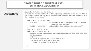
18. DIJKSTRA’S ALGORITHM
Example: Relaxation Formula:
If dist[z] > dist[u] + w[u,z], then
dist[z] = dist[u] + w[u,z]

19. MINIMUM SPANNING TREE
• A spanning tree is defined as a subgraph of an undirected graph in which
all the vertices are connected.
• A tree consisting of all the vertices of a graph is called a spanning tree.
• The weight of spanning tree for a weighted graph is the sum of all the
edge weights.
• The spanning tree with minimum total weight is called the minimum
spanning tree(MST).
• MST is a minimal graph G’ of a graph G, such that
V(G’) = V(G) and E(G’)⊆ 𝐸(𝐺)
• If there are N vertices in the graph, then the MST contains (N-1) edges.

20. MINIMUM SPANNING TREE
a d
b c
a d
b c
a d
b c
a d
b c
a d
b c
a d
b c
a d
b c
a d
b c
2
3
4
5
6

21. MINIMUM SPANNING TREE
a d
b c
a d
b c
a d
b c
a d
b c
a d
b c
a d
b c
a d
b c
a d
b c
2
3
4
5
6
MST

22. MINIMUM SPANNING TREE
The following are the two different algorithms to find out the MST:
1. Prim’s Algorithm
2. Kruskal’s Algorithm

23. PRIM’S ALGORITHM
• Prim’s algorithm starts by selecting a node arbitrarily.
• Prim’s algorithm builds the MST by iteratively adding nodes into a working tree.
• A tree on n nodes has n-1 edges.
• Steps for finding MST using Prim’s:
1. Start with a tree which contains only one node.
2. Identify a node(outside the tree) which is closest to the tree and add the minimum
cost edge from that node to some node in the tree and incorporate additional node as
a part of the tree.
3. If there are less than n-1 edges in the tree, go to step 2.

24. PRIM’S ALGORITHM
Example 1:

25. PRIM’S ALGORITHM
Example 2:

26. PRIM’S ALGORITHM

27. PRIM’S ALGORITHM
https://somaiya0-
my.sharepoint.com/:w:/g/personal/gopal_s_somaiya_edu/EaGquP2a38ROiwUBg1izvZMB-
ONtu90-tIjlUuAlMWlMaA?e=WhtPgA

28. KRUSKAL’S ALGORITHM
• Developed by Joseph Kruskal in 1957.
• The Kruskal’s algorithm creates the MST “T” by adding the edges with minimum cost
one at a time to T.
• A minimum cost spanning tree T is built edge by edge without forming the cycle.
• Start with the edge of minimum cost.
• If there are several edges with the same minimum cost, then we select any one of them
and add it to the spanning tree T provided its addition does not form a cycle.
• Then add an edge with the next lowest cost and so on.

29. KRUSKAL’S ALGORITHM
• Repeat this process until we have selected N–1 edges to form the complete MST.
• Edges can only be added if they do not form a cycle.
• In Kruskal’s Algorithm, edges are considered in nondecreasing order of their costs.
• In contrast to Prim’s, there may be forest at different stages of the algorithm, which
get converted into tree

30. KRUSKAL’S ALGORITHM
Algorithm Kruskal
tree = ∅;
While((tree has less than n-1 edges) && (E≠ ∅))
{
select an edge (u,v) from E of lowest cost;
remove(u,v) from E;
if((u,v) does not create a cycle in tree)
add(u,v) to tree;
else
discard(u,v);
}

31. KRUSKAL’S ALGORITHM

32. KRUSKAL’S ALGORITHM