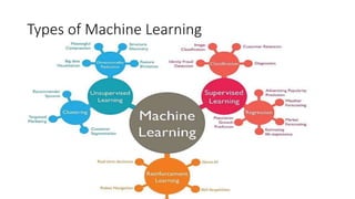
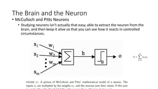
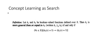
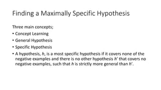
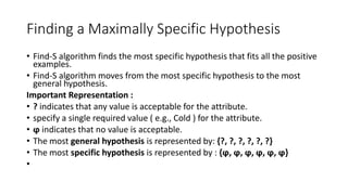
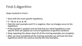
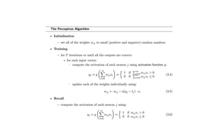
The document discusses machine learning techniques and concepts such as supervised learning, linear discriminant analysis, perceptrons, and more. It begins by defining machine learning and different types including supervised learning. It then covers topics like the brain and neurons, concept learning as search, finding maximally specific hypotheses, version spaces, and the candidate elimination algorithm. It also discusses linear discriminants, perceptrons, and applications of machine learning.

1. Machine Learning Techniques
M. Lilly Florence
Adhiyamaan College of Engineering
Hosur

2. Content
• Learning
• Types of Machine Learning
• Supervised Learning
• The Brain and the Neuron
• Design a Learning System
• Perspectives and Issues in Machine Learning
• Concept Learning as Task
• Concept Learning as Search
• Finding a Maximally Specific Hypothesis
• Version Spaces and the Candidate Elimination Algorithm
• Linear Discriminants
• Perceptron
• Linear Separability
• Linear Regression

3. Learning
• It is said that the term machine learning was first coined by Arthur Lee
Samuel, a pioneer in the AI field, in 1959.
• “Machine learning is the field of study that gives computers the ability
to learn without being explicitly programmed. — Arthur L. Samuel,
AI pioneer, 1959”.
• A computer program is said to learn from experience E with respect to
some class of tasks T and performance measure P, if its performance at
tasks in T, as measured by P, improves with experience E. — Tom
Mitchell, Machine Learning Professor at Carnegie Mellon University
• To illustrate this quote with an example, consider the problem of
recognizing handwritten digits:
• Task T: classifying handwritten digits from images
• Performance measure P : percentage of digits classified correctly
• Training experience E: dataset of digits given classifications,

4. Why “Learn” ?
4
• Machine learning is programming computers to optimize a
performance criterion using example data or past experience.
• There is no need to “learn” to calculate payroll
• Learning is used when:
• Human expertise does not exist (navigating on Mars),
• Humans are unable to explain their expertise (speech recognition)
• Solution changes in time (routing on a computer network)
• Solution needs to be adapted to particular cases (user biometrics)

5. Basic components of learning process
• Four components, namely, data storage, abstraction, generalization and
evaluation.
• 1. Data storage - Facilities for storing and retrieving huge amounts of data
are an important component of the learning process
• 2. Abstraction - Abstraction is the process of extracting knowledge about
stored data. This involves creating general concepts about the data as a
whole. The creation of knowledge involves application of known models
and creation of new models. The process of fitting a model to a dataset is
known as training. When the model has been trained, the data is
transformed into an abstract form that summarizes the original
information.
• 3. Generalization - The term generalization describes the process of turning
the knowledge about stored data into a form that can be utilized for future
action.
• 4. Evaluation - It is the process of giving feedback to the user to measure
the utility of the learn

6. Learning Model
• The basic idea of Learning models has divided into three categories.
• Using a Logical expression. (Logical models)
• Using the Geometry of the instance space. (Geometric models)
• Using Probability to classify the instance space. (Probabilistic models

7. Applications of Machine Learning
• Email spam detection
• Face detection and matching (e.g., iPhone X)
• Web search (e.g., DuckDuckGo, Bing, Google)
• Sports predictions
• Post office (e.g., sorting letters by zip codes)
• ATMs (e.g., reading checks)
• Credit card fraud
• Stock predictions
• Smart assistants (Apple Siri, Amazon Alexa, . . . )
• Product recommendations (e.g., Netflix, Amazon)
• Self-driving cars (e.g., Uber, Tesla)
• Language translation (Google translate)
• Sentiment analysis
• Drug design
• Medical diagnose

8. Types of Machine Learning
• The three broad categories of machine learning are summarized in
the following figure:
• Supervised learning
• Unsupervised learning and
• Reinforcement learning
• Evolutionary learning

9. Types of Machine Learning

10. Supervised learning
• Supervised learning is the subcategory of machine learning that
focuses on learning a classification or regression model, that is,
learning from labeled training data.
• Classification
• Regression

12. The Brain and the Neuron
• Brain
• Nerve Cell-Neuron
• Each neuron is typically connected to thousands of other neurons, so that it is
estimated that there are about 100 trillion (= 1014) synapses within the brain.
After firing, the neuron must wait for some time to recover its energy (the
refractory period) before it can fire again
• Hebb’s Rule - rule says that the changes in the strength of synaptic connections
are proportional to the correlation in the firing of the two connecting neurons. So
if two neurons consistently fire simultaneously, then any connection between
them will change in strength, becoming stronger.
• There are other names for this idea that synaptic connections between neurons
and assemblies of neurons can be formed when they fire together and can
become stronger. It is also known as long-term potentiation and neural plasticity,
and it does appear to have correlates in real brains.

13. The Brain and the Neuron
• McCulloch and Pitts Neurons
• Studying neurons isn’t actually that easy, able to extract the neuron from the
brain, and then keep it alive so that you can see how it reacts in controlled
circumstances.

14. Designing a Learning System
• The design choices has the following key components:
1. Type of training experience – Direct/Indirect,
Supervised/Unsupervised
2. Choosing the Target Function
3. Choosing a representation for the Target Function
4. Choosing an approximation algorithm for the Target Function
5. The final Design

15. Designing a Learning System
Real-world examples of machine learning problems include
“Is this cancer?”,
“What is the market value of this house?”,
“Which of these people are good friends with each other?”,
“Will this rocket engine explode on take off?”,
“Will this person like this movie?”,
“Who is this?”, “What did you say?”, and
“How do you fly this thing?” All of these problems are excellent targets for
an ML project; in fact ML has been applied to each of them with great
success.

17. PERSPECTIVES AND ISSUES IN MACHINE
LEARNING
Issues in Machine Learning
• What algorithms exist for learning general target functions from specific training examples? In what
settings will particular algorithms converge to the desired function, given sufficient training data? Which
algorithms perform best for which types of problems and representations?
• How much training data is sufficient? What general bounds can be found to relate the confidence in
learned hypotheses to the amount of training experience and the character of the learner's hypothesis space?
• When and how can prior knowledge held by the learner guide the process of generalizing from examples?
Can prior knowledge be helpful even when it is only approximately correct?
• What is the best strategy for choosing a useful next training experience, and how does the choice of this
strategy alter the complexity of the learning problem?
• What is the best way to reduce the learning task to one or more function approximation problems? Put
another way, what specific functions should the system attempt to learn? Can this process itself be automated?
• How can the learner automatically alter its representation to improve its ability to represent and learn the
target function?

18. Enjoysport examples

19. Concept Learning as Search
• The goal of this search is to find the hypothesis that best fits the
training examples.
• By selecting a hypothesis representation, the designer of the learning
algorithm implicitly defines the space of all hypotheses that the
program can ever represent and therefore can ever learn.
• Consider, for example,the instances X and hypotheses H in the
EnjoySport learning task. In learning as a search problem, it is natural
that our study of learning algorithms will examine the different
strategies for searching the hypothesis space.

20. Concept Learning as Search
• General-to-Specific Ordering of Hypotheses
• To illustrate the general-to-specific ordering, consider the two
hypotheses
• h1 = (Sunny, ?, ?, Strong, ?, ?)
• h2=(Sunny,?,?,?,?,?)
• Now consider the sets of instances that are classified positive by hl
and by h2. Because h2 imposes fewer constraints on the instance, it
classifies more instances as positive. In fact, any instance classified
positive by h1 will also be classified positive by h2. Therefore, we say
that h2 is more general than h1.
• First, for any instance x in X and hypothesis h in H, we say that x
satisfies h if and only if h(x) = 1

21. Concept Learning as Search
•

22. Finding a Maximally Specific Hypothesis
Three main concepts;
• Concept Learning
• General Hypothesis
• Specific Hypothesis
• A hypothesis, h, is a most specific hypothesis if it covers none of the
negative examples and there is no other hypothesis h′ that covers no
negative examples, such that h is strictly more general than h′.

23. Finding a Maximally Specific Hypothesis
• Find-S algorithm finds the most specific hypothesis that fits all the positive
examples.
• Find-S algorithm moves from the most specific hypothesis to the most
general hypothesis.
Important Representation :
• ? indicates that any value is acceptable for the attribute.
• specify a single required value ( e.g., Cold ) for the attribute.
• ϕ indicates that no value is acceptable.
• The most general hypothesis is represented by: {?, ?, ?, ?, ?, ?}
• The most specific hypothesis is represented by : {ϕ, ϕ, ϕ, ϕ, ϕ, ϕ}
•

24. Find-S Algorithm
Steps Involved In Find-S :
• Start with the most specific hypothesis.
• h = {ϕ, ϕ, ϕ, ϕ, ϕ, ϕ}
• Take the next example and if it is negative, then no changes occur to the
hypothesis.
• If the example is positive and we find that our initial hypothesis is too
specific then we update our current hypothesis to general condition.
• Keep repeating the above steps till all the training examples are complete.
• After we have completed all the training examples we will have the final
hypothesis which can used to classify the new examples.

26. • First we consider the hypothesis to be more specific hypothesis. Hence, our hypothesis
would be :
h = {ϕ, ϕ, ϕ, ϕ, ϕ, ϕ}
• Consider example 1 :
• The data in example 1 is { GREEN, HARD, NO, WRINKLED }. We see that our initial
hypothesis is more specific and we have to generalize it for this example. Hence, the
hypothesis becomes :
h = { GREEN, HARD, NO, WRINKLED }
• Consider example 2 :
Here we see that this example has a negative outcome. Hence we neglect this example
and our hypothesis remains the same.
h = { GREEN, HARD, NO, WRINKLED }
•

27. • Consider example 3 :
Here we see that this example has a negative outcome. Hence we neglect this
example and our hypothesis remains the same.
h = { GREEN, HARD, NO, WRINKLED }
• Consider example 4 :
The data present in example 4 is { ORANGE, HARD, NO, WRINKLED }. We compare
every single attribute with the initial data and if any mismatch is found we
replace that particular attribute with general case ( ” ? ” ). After doing the process
the hypothesis becomes :
h = { ?, HARD, NO, WRINKLED }
• Consider example 5 :
The data present in example 5 is { GREEN, SOFT, YES, SMOOTH }. We compare
every single attribute with the initial data and if any mismatch is found we
replace that particular attribute with general case ( ” ? ” ). After doing the process
the hypothesis becomes :
h = { ?, ?, ?, ? }
Since we have reached a point where all the attributes in our hypothesis have the
general condition, the example 6 and example 7 would result in the same
hypothesizes with all general attributes.
h = { ?, ?, ?, ? }
• Hence, for the given data the final hypothesis would be :
Final Hyposthesis: h = { ?, ?, ?, ? }

28. Version Space
• A version space is a hierarchical representation of knowledge that enables
you to keep track of all the useful information supplied by a sequence of
learning examples without remembering any of the examples.
• The version space method is a concept learning process accomplished by
managing multiple models within a version space.
• Definition (Version space). A concept is complete if it covers all positive
examples.
• A concept is consistent if it covers none of the negative examples. The
version space is the set of all complete and consistent concepts. This set is
convex and is fully defined by its least and most general elements.

29. Version Space
To represent the version space is simply to list all of its members. This leads to a simple learning
algorithm, which we might call the LIST-THEN ELIMINATE algorithm
• The LIST-THEN-ELIMINATE algorithm first initializes the version space to contain all hypotheses in H,
then eliminates any hypothesis found inconsistent with any training example.
• The version space of candidate hypotheses thus shrinks as more examples are observed, until ideally just
one hypothesis remains that is consistent with all the observed examples.

30. Version Space

31. Candidate Elimination Learning Algorithm

33. Origin Manufacturer Color Decade Type Example Type
Japan Honda Blue 1980 Economy Positive
Japan Toyota Green 1970 Sports Negative
Japan Toyota Blue 1990 Economy Positive
USA Chrysler Red 1980 Economy Negative
Japan Honda White 1980 Economy Positive
Problem 1:
Learning the concept of "Japanese Economy Car"
Features: ( Country of Origin, Manufacturer, Color, Decade, Type )

34. • Solution:
• 1. Positive Example: (Japan, Honda, Blue, 1980, Economy)
• Initialize G to a singleton set that includes everything.
G = { (?, ?, ?, ?, ?) }
• Initialize S to a singleton set that includes the first positive example.
S = { (Japan, Honda, Blue, 1980, Economy) }

35. Linear Discriminant Analysis
• In 1936, Ronald A.Fisher formulated Linear Discriminant first time and
showed some practical uses as a classifier, it was described for a 2-class
problem, and later generalized as ‘Multi-class Linear Discriminant Analysis’
or ‘Multiple Discriminant Analysis’ by C.R.Rao in the year 1948.
• Linear Discriminant Analysis is the most commonly used dimensionality
reduction technique in supervised learning. Basically, it is a preprocessing
step for pattern classification and machine learning applications.
• It projects the dataset into moderate dimensional-space with a genuine
class of separable features that minimize overfitting and computational
costs.

37. Working of Linear Discriminant Analysis - Assumptions
• Every feature either be variable, dimension, or attribute in the dataset
has gaussian distribution, i.e, features have a bell-shaped curve.
• Each feature holds the same variance, and has varying values around
the mean with the same amount on average.
• Each feature is assumed to be sampled randomly.
• Lack of multicollinearity in independent features and there is an
increment in correlations between independent features and the
power of prediction decreases.

38. LDA achieve this via three step process;
• First step: To compute the separate ability amid various classes,i.e,
the distance between the mean of different classes, that is also
known as between-class variance

39. • Second Step: To compute the distance among the mean and sample
of each class, that is also known as the within class variance.

40. • Third step: To create the lower dimensional space that maximizes the
between class variance and minimizes the within class variance.
• Assuming P as the lower dimensional space projection that is known
as Fisher’s criterion.

41. • For example, LDA can be used as a classification task for speech
recognition, microarray data classification, face recognition, image
retrieval, bioinformatics, biometrics, chemistry, etc.
• https://people.revoledu.com/kardi/tutorial/LDA/Numerical%20Exam
ple.html

42. Perceptron
• Perceptron is a single layer neural network and a multi-layer
perceptron is called Neural Networks.
• Perceptron is a linear classifier (binary). Also, it is used in supervised
learning.

43. The perceptron consists of 4 parts.
• Input values or One input layer
• Weights and Bias
• Net sum
• Activation Function

45. • The perceptron works on these simple steps
a. All the inputs x are multiplied with their weights w. Let’s call it k.

46. b. Add all the multiplied values and call them Weighted Sum.

47. C. Apply that weighted sum to the correct Activation Function.

48. Why do we need Weights and Bias?
• Weights shows the strength of the particular node.
• A bias value allows you to shift the activation function curve up or down.

49. Why do we need Activation Function?
• In short, the activation functions are used to map the input between the
required values like (0, 1) or (-1, 1).