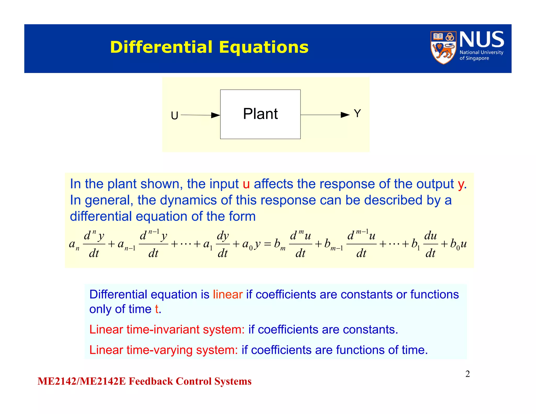
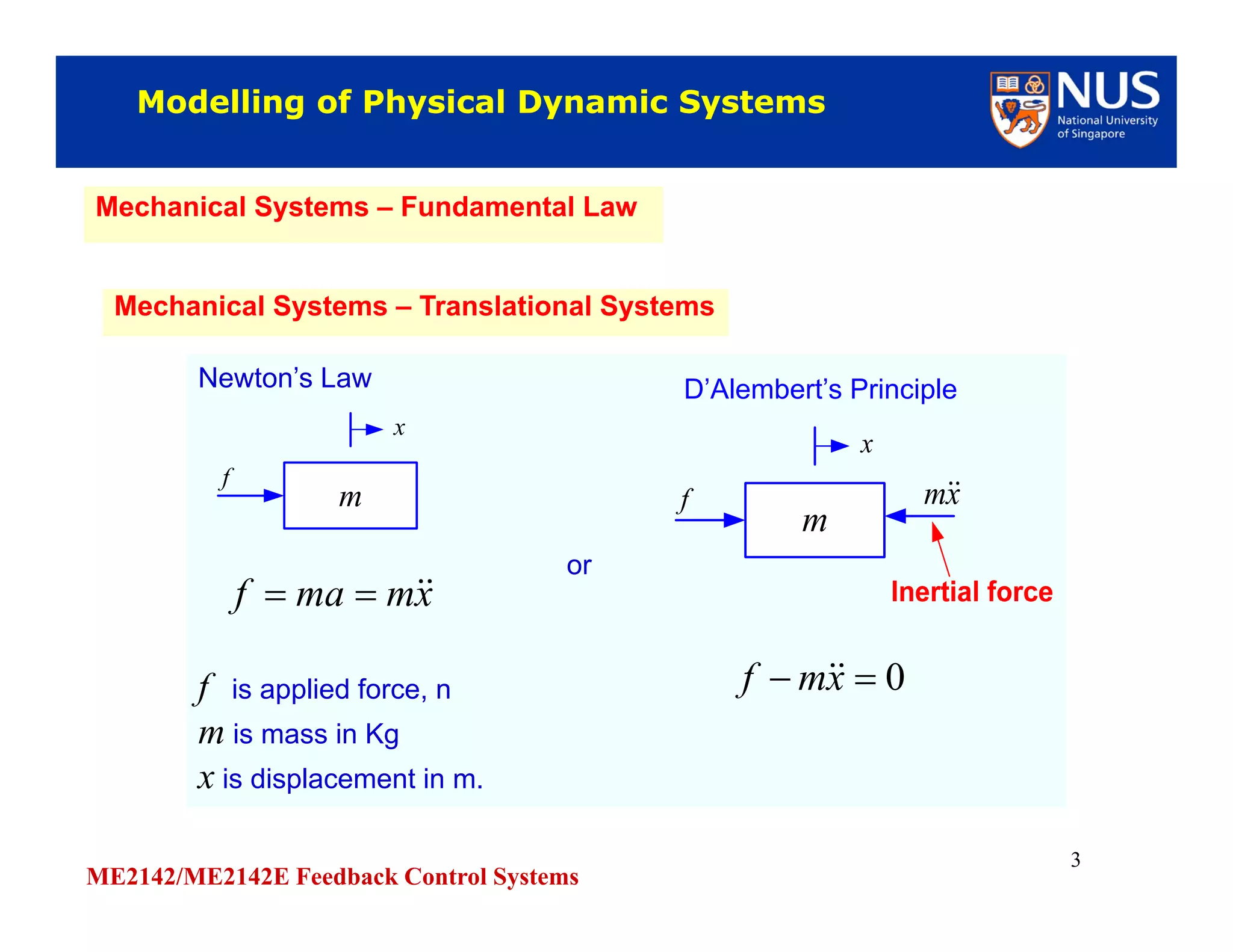
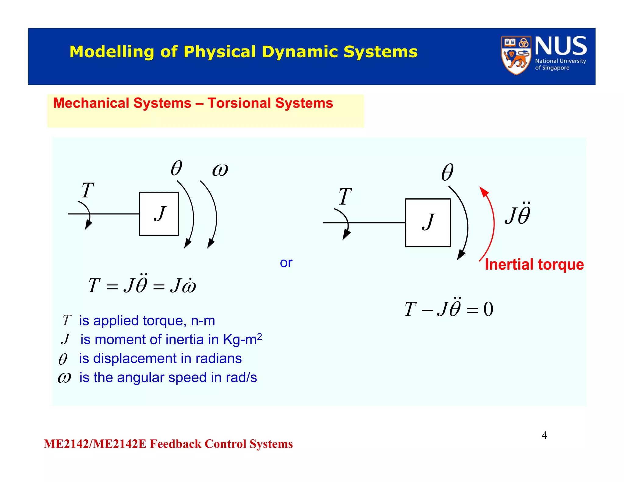
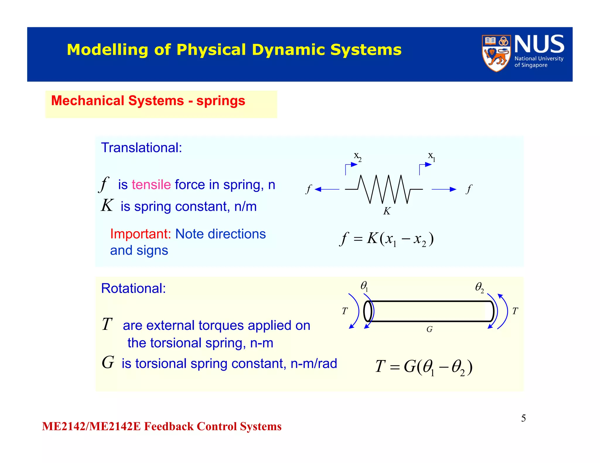
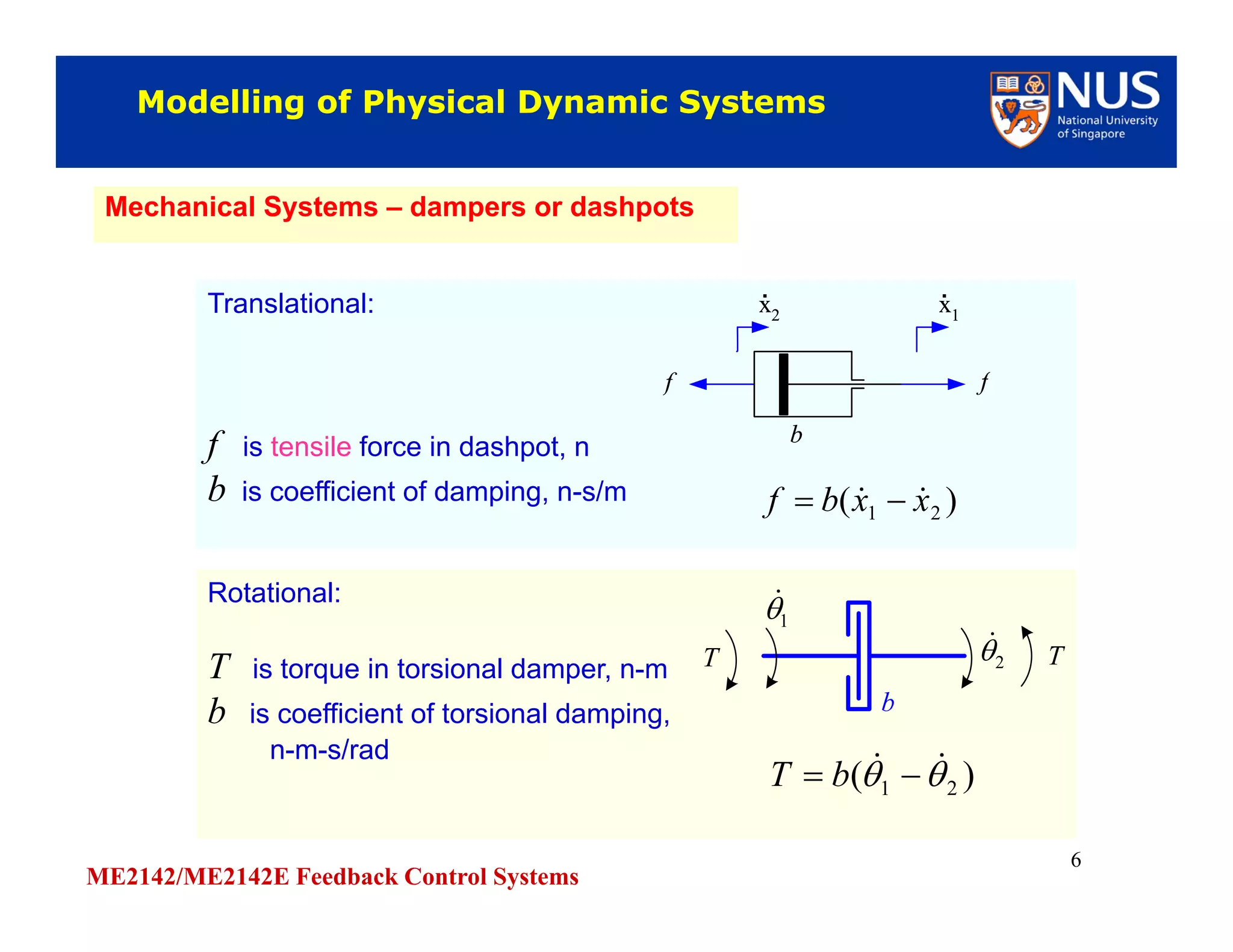
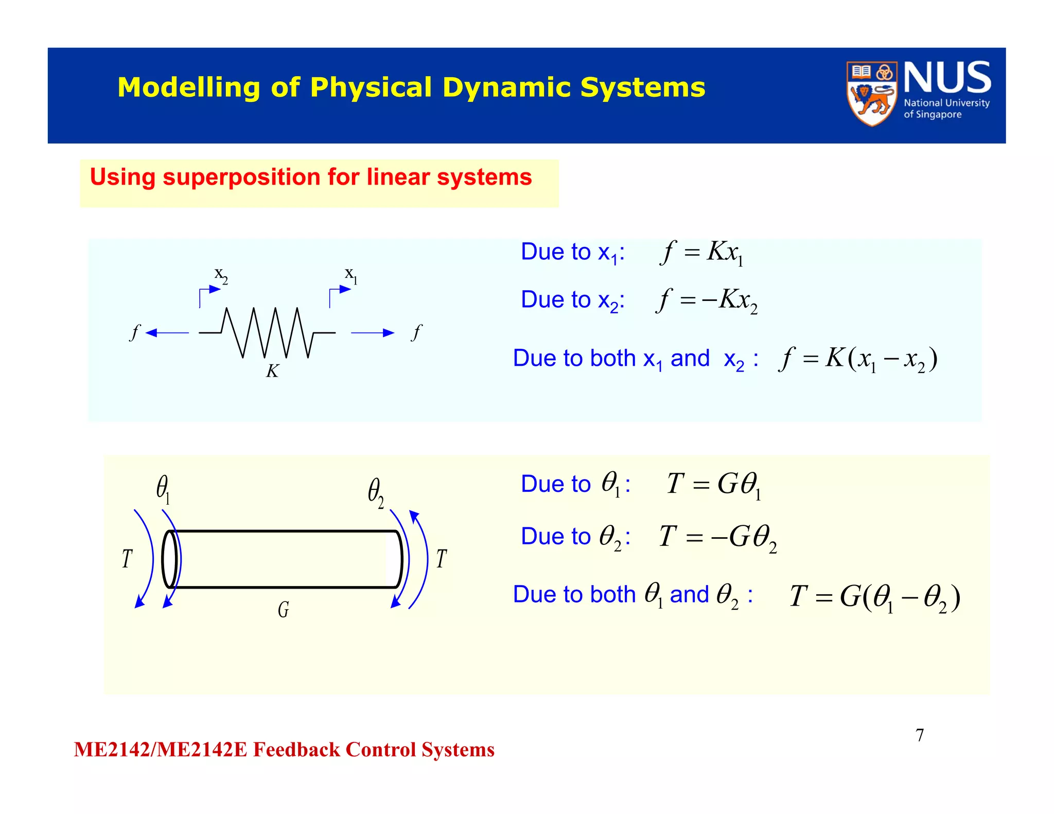
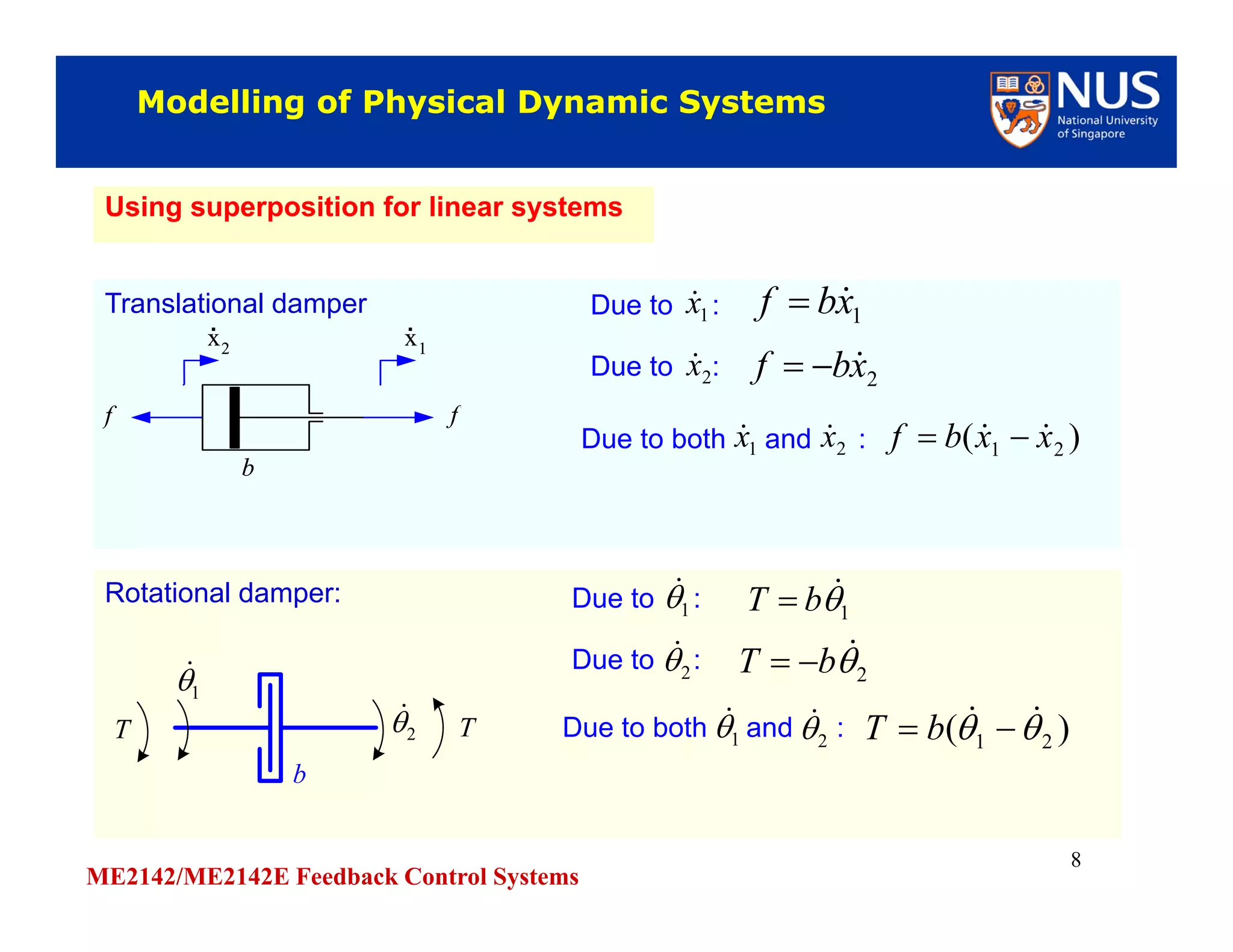
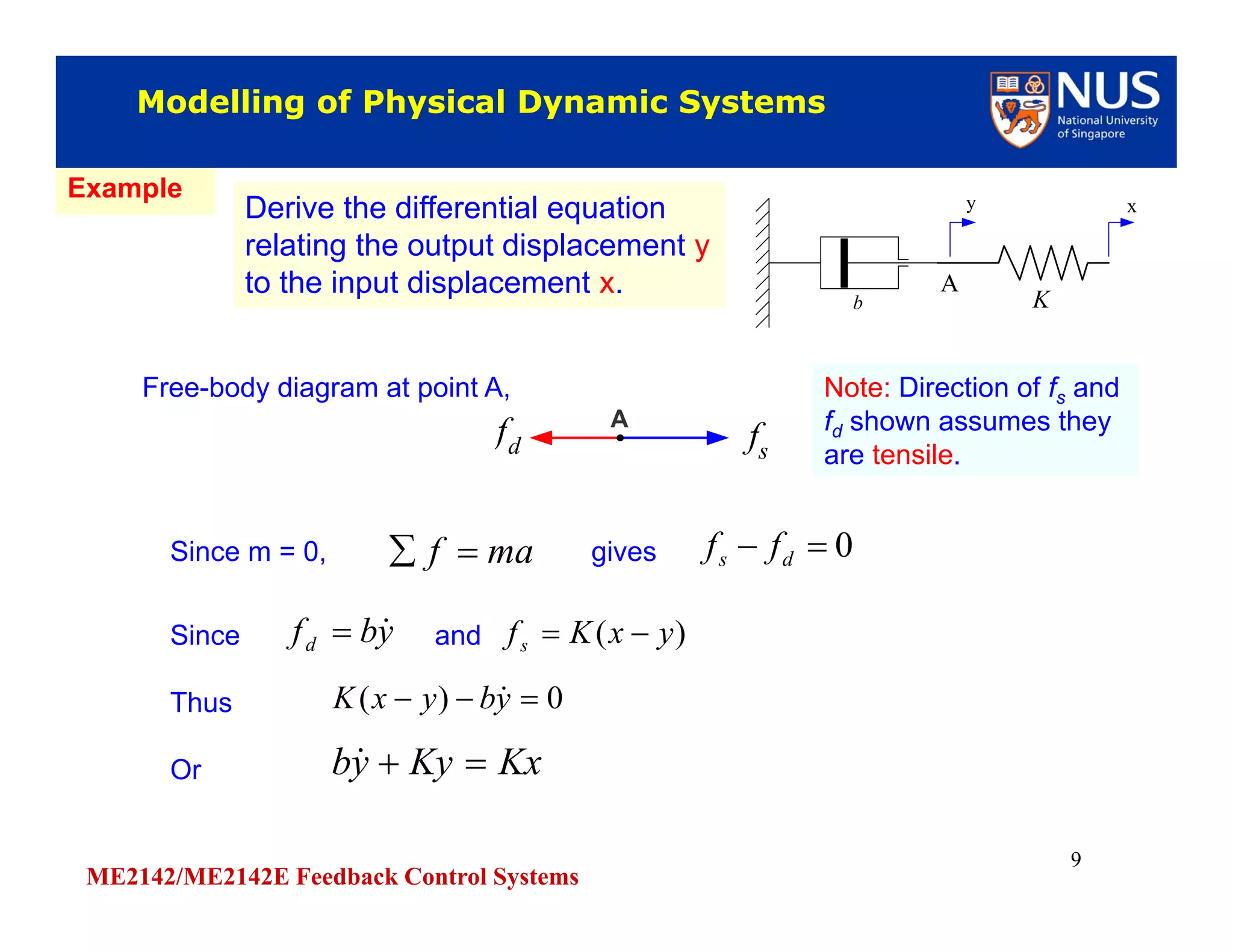
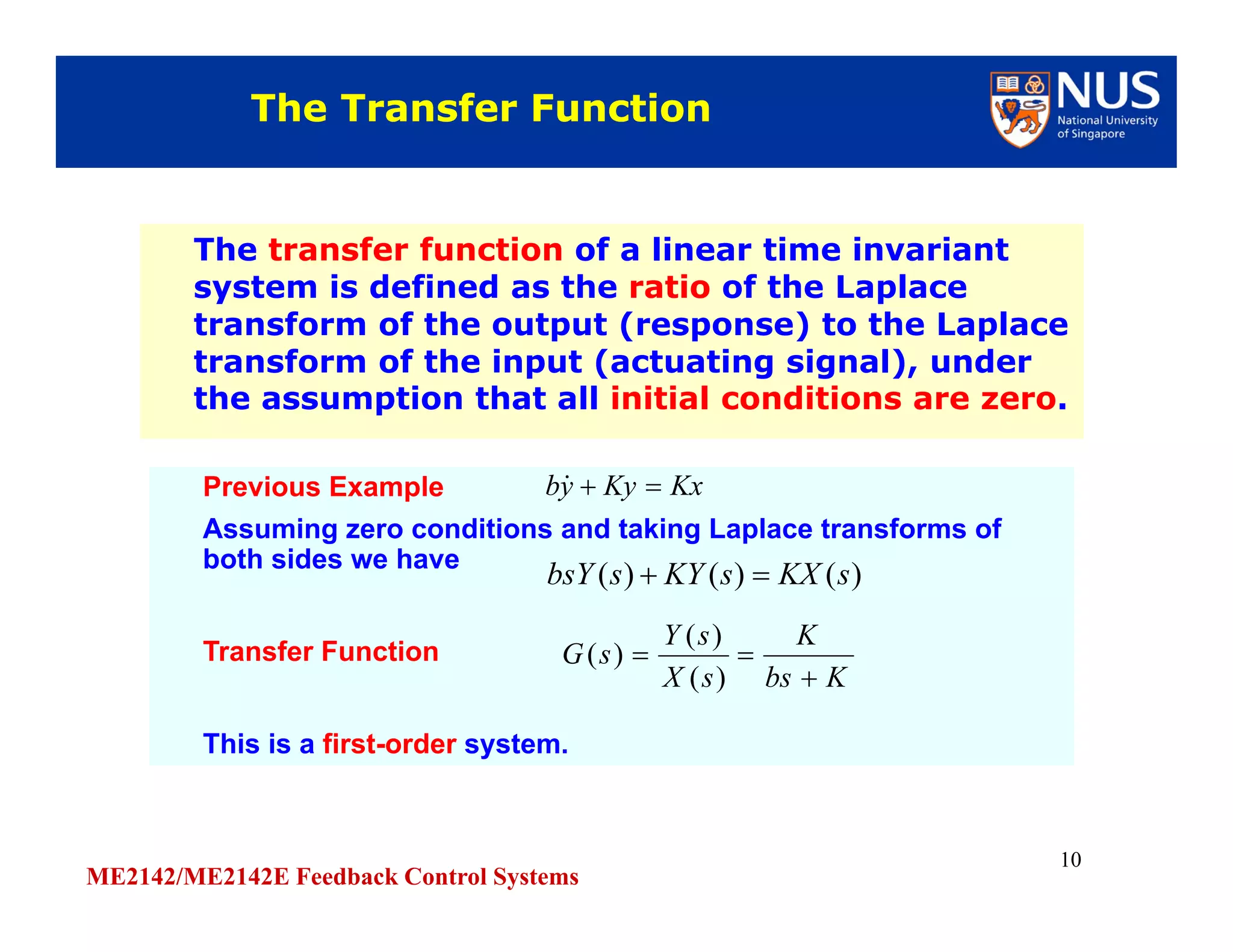
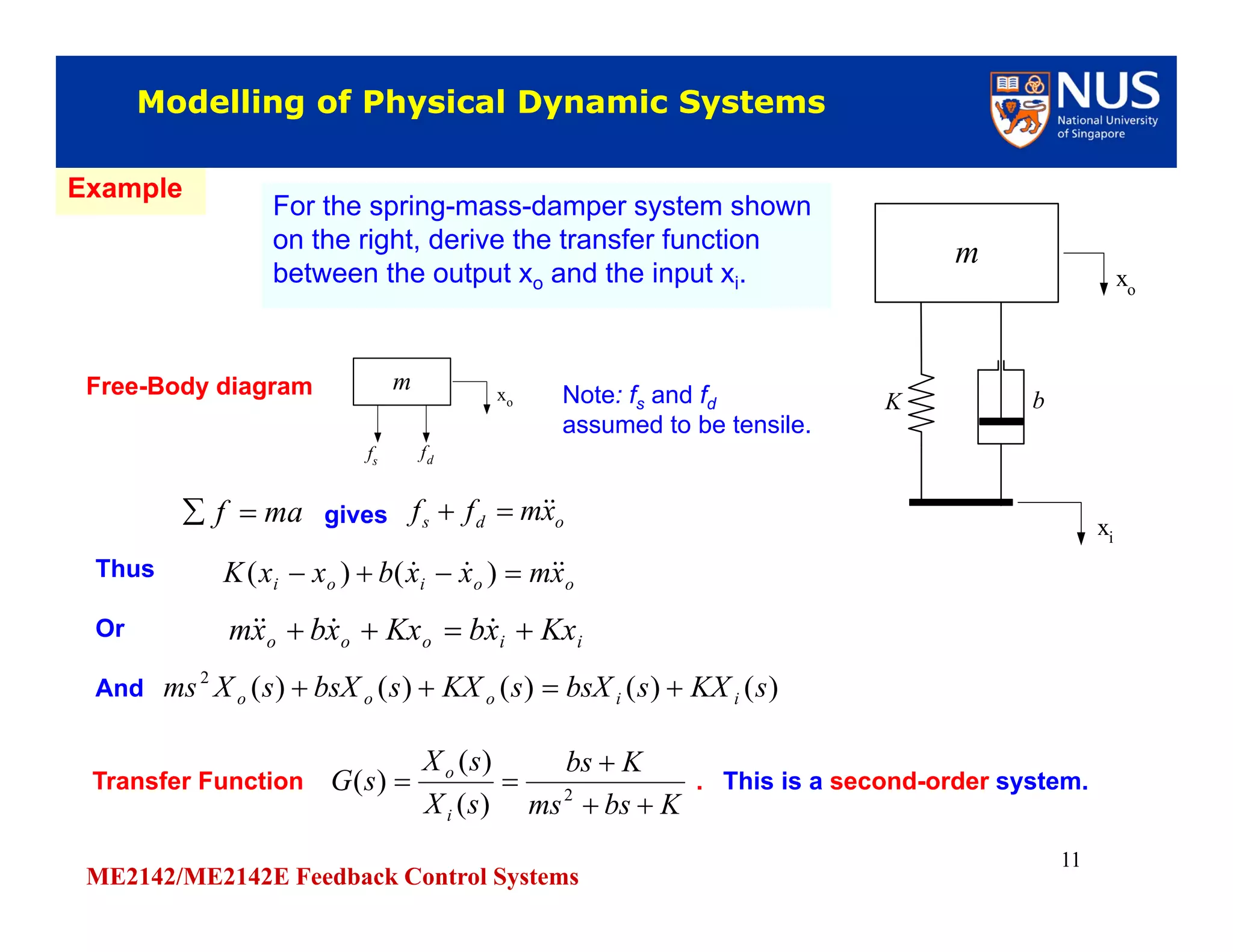
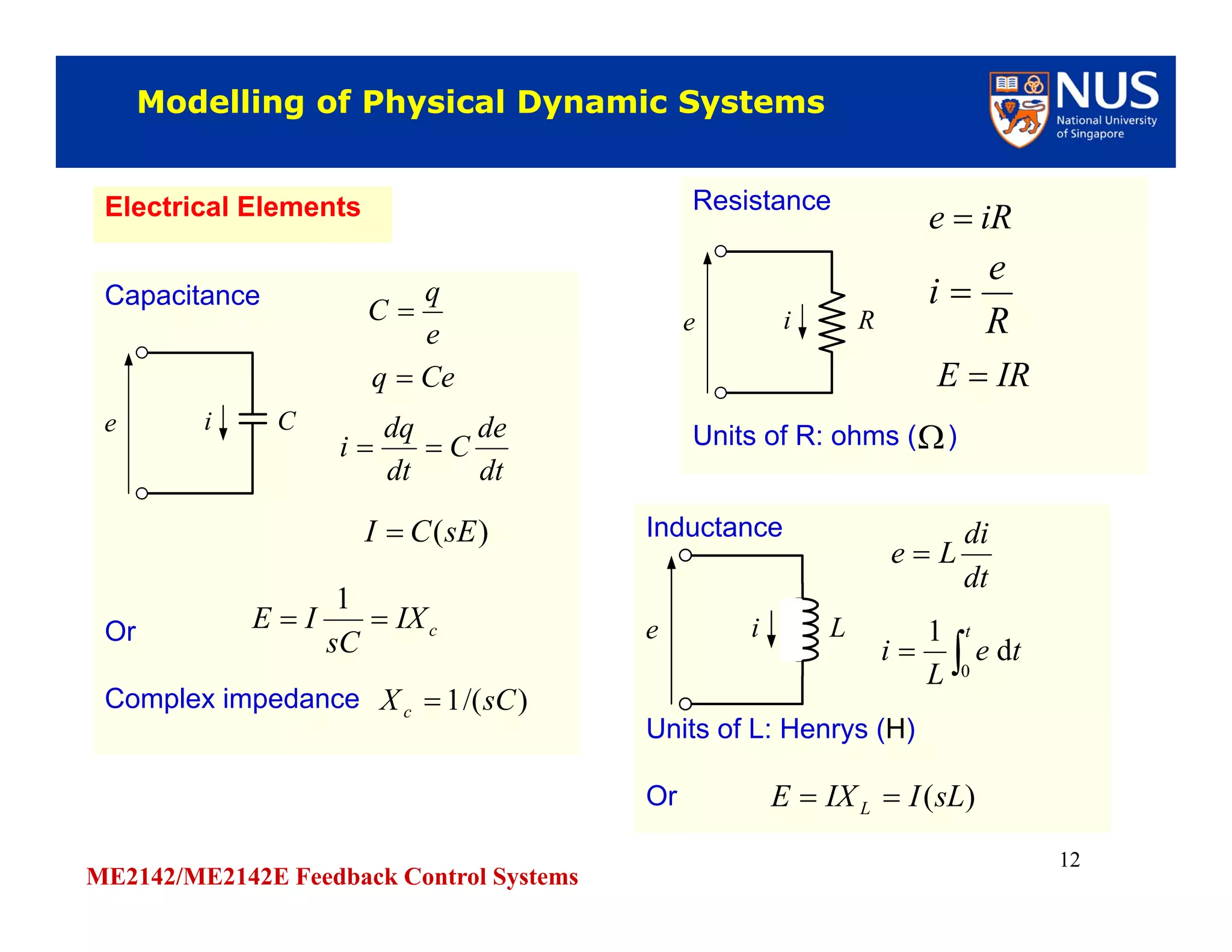
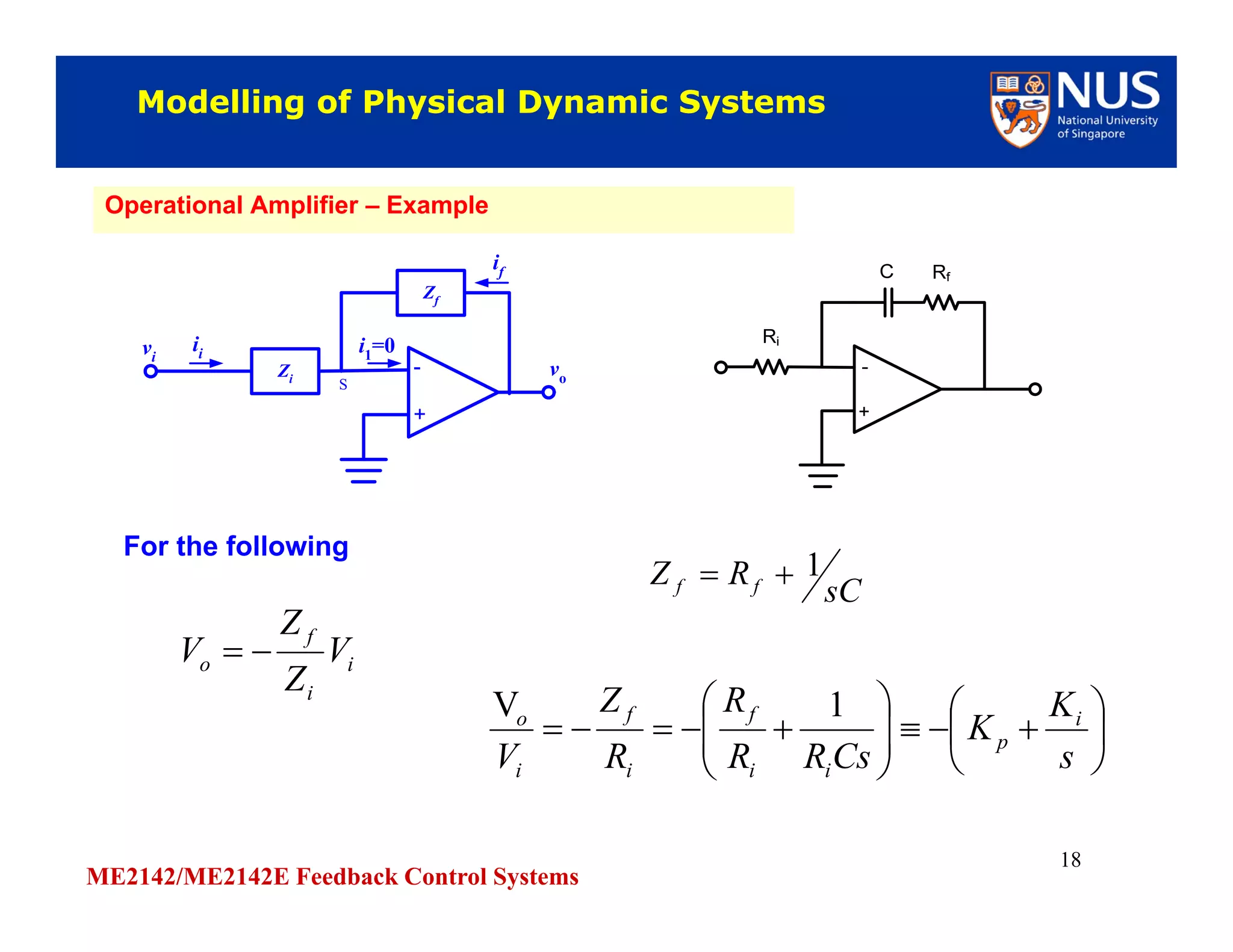
ME2142/ME2142E Feedback Control Systems
1
Modelling of Physical Systems
The Transfer Function
Modelling of Physical Systems
The Transfer Function
ME2142/ME2142E Feedback Control SystemsME2142/ME2142E Feedback Control Systems
ME2142/ME2142E Feedback Control Systems
2
Differential EquationsDifferential Equations
Differential equation is linear if coefficients are constants or functions
only of time t.
Linear time-invariant system: if coefficients are constants.
Linear time-varying system: if coefficients are functions of time.
Differential equation is linear if coefficients are constants or functions
only of time t.
Linear time-invariant system: if coefficients are constants.
Linear time-varying system: if coefficients are functions of time.
PlantU YPlantU Y
In the plant shown, the input u affects the response of the output y.
In general, the dynamics of this response can be described by a
differential equation of the form
In the plant shown, the input u affects the response of the output y.
In general, the dynamics of this response can be described by a
differential equation of the form
ub
dt
du
b
dt
ud
b
dt
ud
bya
dt
dy
a
dt
yd
a
dt
yd
a
m
m
m
m
n
n
n
n 01
1
101
1
1 



 
ME2142/ME2142E Feedback Control Systems
3
Newton’s Law
f is applied force, n
m is mass in Kg
x is displacement in m.
Newton’s Law
f is applied force, n
m is mass in Kg
x is displacement in m.
m
f
x
Mechanical Systems – Translational SystemsMechanical Systems – Translational Systems
Mechanical Systems – Fundamental LawMechanical Systems – Fundamental Law
Modelling of Physical Dynamic SystemsModelling of Physical Dynamic Systems
xmmaf 
or
0 xmf 
xm 
D’Alembert’s Principle
ME2142/ME2142E Feedback Control Systems
4
T is applied torque, n-m
J is moment of inertia in Kg-m2
is displacement in radians
is the angular speed in rad/s
T is applied torque, n-m
J is moment of inertia in Kg-m2
is displacement in radians
is the angular speed in rad/s
J
T



Modelling of Physical Dynamic SystemsModelling of Physical Dynamic Systems
Mechanical Systems – Torsional SystemsMechanical Systems – Torsional Systems
  JJT 
0 JT

J
or
ME2142/ME2142E Feedback Control Systems
5
Rotational:
T are external torques applied on
the torsional spring, n-m
G is torsional spring constant, n-m/rad
Rotational:
T are external torques applied on
the torsional spring, n-m
G is torsional spring constant, n-m/rad
1 2
Translational:
f is tensile force in spring, n
K is spring constant, n/m
Translational:
f is tensile force in spring, n
K is spring constant, n/m
f
x1
x2
f
K
Modelling of Physical Dynamic SystemsModelling of Physical Dynamic Systems
Mechanical Systems - springsMechanical Systems - springs
)( 21 xxKf Important: Note directions
and signs
)( 21   GT
ME2142/ME2142E Feedback Control Systems
6
Translational:
f is tensile force in dashpot, n
b is coefficient of damping, n-s/m
Translational:
f is tensile force in dashpot, n
b is coefficient of damping, n-s/m
f
x1x2
f
.
b
.
f
x1x2
f
.
b
.
Modelling of Physical Dynamic SystemsModelling of Physical Dynamic Systems
Mechanical Systems – dampers or dashpotsMechanical Systems – dampers or dashpots
)( 21 xxbf  
Rotational:
T is torque in torsional damper, n-m
b is coefficient of torsional damping,
n-m-s/rad
Rotational:
T is torque in torsional damper, n-m
b is coefficient of torsional damping,
n-m-s/rad
2
1
)( 21    bT
ME2142/ME2142E Feedback Control Systems
7
1 2
f
x1
x2
f
K
Modelling of Physical Dynamic SystemsModelling of Physical Dynamic Systems
Using superposition for linear systemsUsing superposition for linear systems
Due to x1: 1Kxf 
2Kxf Due to x2:
)( 21 xxKf Due to both x1 and x2 :
2GT Due to :2
Due to : 1GT 1
)( 21   GTDue to both and :1 2
ME2142/ME2142E Feedback Control Systems
8
Translational damperTranslational damper
f
x1x2
f
.
b
.
f
x1x2
f
.
b
.
Modelling of Physical Dynamic SystemsModelling of Physical Dynamic Systems
Rotational damper:Rotational damper:
2
1
Using superposition for linear systemsUsing superposition for linear systems
Due to : 1xbf 1x
Due to :2x 2xbf 
)( 21 xxbf  Due to both and :1x 2x
2bT Due to :2
Due to : 1bT 1
)( 21    bTDue to both and :1
2
ME2142/ME2142E Feedback Control Systems
9
Modelling of Physical Dynamic SystemsModelling of Physical Dynamic Systems
ExampleExample
Since m = 0, givesmaf  0 ds ff
Since and
Thus
Or
ybfd
 )( yxKfs 
0)(  ybyxK 
KxKyyb 
xy
b K
A
Derive the differential equation
relating the output displacement y
to the input displacement x.
Derive the differential equation
relating the output displacement y
to the input displacement x.
Free-body diagram at point A,
A
fs
fd
Note: Direction of fs and
fd shown assumes they
are tensile.
Note: Direction of fs and
fd shown assumes they
are tensile.
ME2142/ME2142E Feedback Control Systems
10
The transfer function of a linear time invariant
system is defined as the ratio of the Laplace
transform of the output (response) to the Laplace
transform of the input (actuating signal), under
the assumption that all initial conditions are zero.
The transfer function of a linear time invariant
system is defined as the ratio of the Laplace
transform of the output (response) to the Laplace
transform of the input (actuating signal), under
the assumption that all initial conditions are zero.
The Transfer FunctionThe Transfer Function
Previous Example
Assuming zero conditions and taking Laplace transforms of
both sides we have
Transfer Function
This is a first-order system.
Previous Example
Assuming zero conditions and taking Laplace transforms of
both sides we have
Transfer Function
This is a first-order system.
KxKyyb 
)()()( sKXsKYsbsY 
Kbs
K
sX
sY
sG


)(
)(
)(
ME2142/ME2142E Feedback Control Systems
11
Modelling of Physical Dynamic SystemsModelling of Physical Dynamic Systems
ExampleExample
Free-Body diagram
givesmaf  ods xmff 
m
fs
fd
xo
m
K b
xi
xo
)()()()()(2
sKXsbsXsKXsbsXsXms iiooo 
ooioi xmxxbxxK   )()(
iiooo KxxbKxxbxm  
Thus
Or
And
Kbsms
Kbs
sX
sX
sG
i
o


 2
)(
)(
)(Transfer Function . This is a second-order system.
For the spring-mass-damper system shown
on the right, derive the transfer function
between the output xo and the input xi.
For the spring-mass-damper system shown
on the right, derive the transfer function
between the output xo and the input xi.
Note: fs and fd
assumed to be tensile.
ME2142/ME2142E Feedback Control Systems
12
Capacitance
Or
Complex impedance
Capacitance
Or
Complex impedance
e
q
C 
Ceq 
dt
de
C
dt
dq
i 
)(sECI 
)/(1 sCXc 
cIX
sC
IE 
1
e i C
Modelling of Physical Dynamic SystemsModelling of Physical Dynamic Systems
Electrical ElementsElectrical Elements Resistance
Units of R: ohms ( )
Resistance
Units of R: ohms ( )
iRe 
R
e
i 

e i R
Inductance
Units of L: Henrys (H)
Or
Inductance
Units of L: Henrys (H)
Or
dt
di
Le 

t
te
L
i
0
d
1
)(sLIIXE L 
e i L
IRE 
ME2142/ME2142E Feedback Control Systems
13
Modelling of Physical Dynamic SystemsModelling of Physical Dynamic Systems
Electrical Circuits- Kirchhoff’s LawsElectrical Circuits- Kirchhoff’s Laws
Current Law:
The sum of currents entering a node is
equal to that leaving it.
Current Law:
The sum of currents entering a node is
equal to that leaving it.
0i
Voltage Law:
The sum algebraic sum of voltage drops
around a closed loop is zero.
Voltage Law:
The sum algebraic sum of voltage drops
around a closed loop is zero.
0e
ME2142/ME2142E Feedback Control Systems
14
Modelling of Physical Dynamic SystemsModelling of Physical Dynamic Systems
Electrical Circuits- ExamplesElectrical Circuits- Examples
RC circuit: Derive the transfer function for the circuit shown,
and
giving
This is a first-order transfer function.
RC circuit: Derive the transfer function for the circuit shown,
and
giving
This is a first-order transfer function.
ci IXIRE 
co IXE 
)/(1
)/(1
sCR
sC
XR
X
E
E
c
c
i
o




1
1


RCs
ei
i C
R
eo
ME2142/ME2142E Feedback Control Systems
15
Modelling of Physical Dynamic SystemsModelling of Physical Dynamic Systems
Electrical Circuits- ExamplesElectrical Circuits- Examples
RLC circuit:
and
giving
This is a second-order transfer function.
RLC circuit:
and
giving
This is a second-order transfer function.
cLi IXIXIRE 
co IXE 
)/(1
)/(1
sCsLR
sC
XXR
X
E
E
cL
c
i
o




1
1
2


RCsLCs
ei
i C
R
eo
L
ME2142/ME2142E Feedback Control Systems
16
Modelling of Physical Dynamic SystemsModelling of Physical Dynamic Systems
Operational Amplifier – Properties of an ideal Op AmpOperational Amplifier – Properties of an ideal Op Amp
Gain A is normally very large so that compared with
other values, is assumed small, equal to zero.
Gain A is normally very large so that compared with
other values, is assumed small, equal to zero.
)( 12 vvAvo 
)( 12 vv 
The input impedance of the Op Amp is usually very high (assumed infinity)
so that the currents i1 and i2 are very small, assumed zero.
The input impedance of the Op Amp is usually very high (assumed infinity)
so that the currents i1 and i2 are very small, assumed zero.
Two basic equation governing the operation of the Op Amp
and
Two basic equation governing the operation of the Op Amp
and 0,0 21  ii2112 or0)( vvvv 
ME2142/ME2142E Feedback Control Systems
17
Modelling of Physical Dynamic SystemsModelling of Physical Dynamic Systems
Operational Amplifier – ExampleOperational Amplifier – Example
For the Op Amp, assume i1=0 and vs=v+=0.For the Op Amp, assume i1=0 and vs=v+=0.
-
+
vi
i1
=0
voZi
Zf
ii
if
S
Then orThen or0 fi ii 0
f
o
i
i
Z
V
Z
V
ThereforeTherefore
i
f
i
o
Z
Z
sV
sV

)(
)(
i
i
f
o V
R
Z
V 
ME2142/ME2142E Feedback Control Systems
18
Modelling of Physical Dynamic SystemsModelling of Physical Dynamic Systems
Operational Amplifier – ExampleOperational Amplifier – Example
-
+
vi
i1
=0
voZi
Zf
ii
if
S
i
i
f
o V
Z
Z
V 
For the following
sC
RZ ff
1













s
K
K
CsRR
R
R
Z
V
i
p
ii
f
i
f
i
o 1V
ME2142/ME2142E Feedback Control Systems
19
Permanent Magnet DC Motor Driving a LoadPermanent Magnet DC Motor Driving a Load
For the dc motor, the back emf is proportional to speed and is given by
where is the voltage constant. The torque produced is proportional to
armature current and is given by where is the torque constant.
For the dc motor, the back emf is proportional to speed and is given by
where is the voltage constant. The torque produced is proportional to
armature current and is given by where is the torque constant.
eK
eK
iKT t tK
Relevant equations:Relevant equations: eaa K
dt
di
LiRe 
iKT t 

b
dt
d
JT 
e i
Ra
La
eK J
b
T

Note: By considering power in = power out, can show that Ke=KtNote: By considering power in = power out, can show that Ke=Kt
ME2142/ME2142E Feedback Control Systems
20
End

3 modelling of physical systems

  • 1.
    ME2142/ME2142E Feedback ControlSystems 1 Modelling of Physical Systems The Transfer Function Modelling of Physical Systems The Transfer Function ME2142/ME2142E Feedback Control SystemsME2142/ME2142E Feedback Control Systems
  • 2.
    ME2142/ME2142E Feedback ControlSystems 2 Differential EquationsDifferential Equations Differential equation is linear if coefficients are constants or functions only of time t. Linear time-invariant system: if coefficients are constants. Linear time-varying system: if coefficients are functions of time. Differential equation is linear if coefficients are constants or functions only of time t. Linear time-invariant system: if coefficients are constants. Linear time-varying system: if coefficients are functions of time. PlantU YPlantU Y In the plant shown, the input u affects the response of the output y. In general, the dynamics of this response can be described by a differential equation of the form In the plant shown, the input u affects the response of the output y. In general, the dynamics of this response can be described by a differential equation of the form ub dt du b dt ud b dt ud bya dt dy a dt yd a dt yd a m m m m n n n n 01 1 101 1 1      
  • 3.
    ME2142/ME2142E Feedback ControlSystems 3 Newton’s Law f is applied force, n m is mass in Kg x is displacement in m. Newton’s Law f is applied force, n m is mass in Kg x is displacement in m. m f x Mechanical Systems – Translational SystemsMechanical Systems – Translational Systems Mechanical Systems – Fundamental LawMechanical Systems – Fundamental Law Modelling of Physical Dynamic SystemsModelling of Physical Dynamic Systems xmmaf  or 0 xmf  xm  D’Alembert’s Principle
  • 4.
    ME2142/ME2142E Feedback ControlSystems 4 T is applied torque, n-m J is moment of inertia in Kg-m2 is displacement in radians is the angular speed in rad/s T is applied torque, n-m J is moment of inertia in Kg-m2 is displacement in radians is the angular speed in rad/s J T    Modelling of Physical Dynamic SystemsModelling of Physical Dynamic Systems Mechanical Systems – Torsional SystemsMechanical Systems – Torsional Systems   JJT  0 JT  J or
  • 5.
    ME2142/ME2142E Feedback ControlSystems 5 Rotational: T are external torques applied on the torsional spring, n-m G is torsional spring constant, n-m/rad Rotational: T are external torques applied on the torsional spring, n-m G is torsional spring constant, n-m/rad 1 2 Translational: f is tensile force in spring, n K is spring constant, n/m Translational: f is tensile force in spring, n K is spring constant, n/m f x1 x2 f K Modelling of Physical Dynamic SystemsModelling of Physical Dynamic Systems Mechanical Systems - springsMechanical Systems - springs )( 21 xxKf Important: Note directions and signs )( 21   GT
  • 6.
    ME2142/ME2142E Feedback ControlSystems 6 Translational: f is tensile force in dashpot, n b is coefficient of damping, n-s/m Translational: f is tensile force in dashpot, n b is coefficient of damping, n-s/m f x1x2 f . b . f x1x2 f . b . Modelling of Physical Dynamic SystemsModelling of Physical Dynamic Systems Mechanical Systems – dampers or dashpotsMechanical Systems – dampers or dashpots )( 21 xxbf   Rotational: T is torque in torsional damper, n-m b is coefficient of torsional damping, n-m-s/rad Rotational: T is torque in torsional damper, n-m b is coefficient of torsional damping, n-m-s/rad 2 1 )( 21    bT
  • 7.
    ME2142/ME2142E Feedback ControlSystems 7 1 2 f x1 x2 f K Modelling of Physical Dynamic SystemsModelling of Physical Dynamic Systems Using superposition for linear systemsUsing superposition for linear systems Due to x1: 1Kxf  2Kxf Due to x2: )( 21 xxKf Due to both x1 and x2 : 2GT Due to :2 Due to : 1GT 1 )( 21   GTDue to both and :1 2
  • 8.
    ME2142/ME2142E Feedback ControlSystems 8 Translational damperTranslational damper f x1x2 f . b . f x1x2 f . b . Modelling of Physical Dynamic SystemsModelling of Physical Dynamic Systems Rotational damper:Rotational damper: 2 1 Using superposition for linear systemsUsing superposition for linear systems Due to : 1xbf 1x Due to :2x 2xbf  )( 21 xxbf  Due to both and :1x 2x 2bT Due to :2 Due to : 1bT 1 )( 21    bTDue to both and :1 2
  • 9.
    ME2142/ME2142E Feedback ControlSystems 9 Modelling of Physical Dynamic SystemsModelling of Physical Dynamic Systems ExampleExample Since m = 0, givesmaf  0 ds ff Since and Thus Or ybfd  )( yxKfs  0)(  ybyxK  KxKyyb  xy b K A Derive the differential equation relating the output displacement y to the input displacement x. Derive the differential equation relating the output displacement y to the input displacement x. Free-body diagram at point A, A fs fd Note: Direction of fs and fd shown assumes they are tensile. Note: Direction of fs and fd shown assumes they are tensile.
  • 10.
    ME2142/ME2142E Feedback ControlSystems 10 The transfer function of a linear time invariant system is defined as the ratio of the Laplace transform of the output (response) to the Laplace transform of the input (actuating signal), under the assumption that all initial conditions are zero. The transfer function of a linear time invariant system is defined as the ratio of the Laplace transform of the output (response) to the Laplace transform of the input (actuating signal), under the assumption that all initial conditions are zero. The Transfer FunctionThe Transfer Function Previous Example Assuming zero conditions and taking Laplace transforms of both sides we have Transfer Function This is a first-order system. Previous Example Assuming zero conditions and taking Laplace transforms of both sides we have Transfer Function This is a first-order system. KxKyyb  )()()( sKXsKYsbsY  Kbs K sX sY sG   )( )( )(
  • 11.
    ME2142/ME2142E Feedback ControlSystems 11 Modelling of Physical Dynamic SystemsModelling of Physical Dynamic Systems ExampleExample Free-Body diagram givesmaf  ods xmff  m fs fd xo m K b xi xo )()()()()(2 sKXsbsXsKXsbsXsXms iiooo  ooioi xmxxbxxK   )()( iiooo KxxbKxxbxm   Thus Or And Kbsms Kbs sX sX sG i o    2 )( )( )(Transfer Function . This is a second-order system. For the spring-mass-damper system shown on the right, derive the transfer function between the output xo and the input xi. For the spring-mass-damper system shown on the right, derive the transfer function between the output xo and the input xi. Note: fs and fd assumed to be tensile.
  • 12.
    ME2142/ME2142E Feedback ControlSystems 12 Capacitance Or Complex impedance Capacitance Or Complex impedance e q C  Ceq  dt de C dt dq i  )(sECI  )/(1 sCXc  cIX sC IE  1 e i C Modelling of Physical Dynamic SystemsModelling of Physical Dynamic Systems Electrical ElementsElectrical Elements Resistance Units of R: ohms ( ) Resistance Units of R: ohms ( ) iRe  R e i   e i R Inductance Units of L: Henrys (H) Or Inductance Units of L: Henrys (H) Or dt di Le   t te L i 0 d 1 )(sLIIXE L  e i L IRE 
  • 13.
    ME2142/ME2142E Feedback ControlSystems 13 Modelling of Physical Dynamic SystemsModelling of Physical Dynamic Systems Electrical Circuits- Kirchhoff’s LawsElectrical Circuits- Kirchhoff’s Laws Current Law: The sum of currents entering a node is equal to that leaving it. Current Law: The sum of currents entering a node is equal to that leaving it. 0i Voltage Law: The sum algebraic sum of voltage drops around a closed loop is zero. Voltage Law: The sum algebraic sum of voltage drops around a closed loop is zero. 0e
  • 14.
    ME2142/ME2142E Feedback ControlSystems 14 Modelling of Physical Dynamic SystemsModelling of Physical Dynamic Systems Electrical Circuits- ExamplesElectrical Circuits- Examples RC circuit: Derive the transfer function for the circuit shown, and giving This is a first-order transfer function. RC circuit: Derive the transfer function for the circuit shown, and giving This is a first-order transfer function. ci IXIRE  co IXE  )/(1 )/(1 sCR sC XR X E E c c i o     1 1   RCs ei i C R eo
  • 15.
    ME2142/ME2142E Feedback ControlSystems 15 Modelling of Physical Dynamic SystemsModelling of Physical Dynamic Systems Electrical Circuits- ExamplesElectrical Circuits- Examples RLC circuit: and giving This is a second-order transfer function. RLC circuit: and giving This is a second-order transfer function. cLi IXIXIRE  co IXE  )/(1 )/(1 sCsLR sC XXR X E E cL c i o     1 1 2   RCsLCs ei i C R eo L
  • 16.
    ME2142/ME2142E Feedback ControlSystems 16 Modelling of Physical Dynamic SystemsModelling of Physical Dynamic Systems Operational Amplifier – Properties of an ideal Op AmpOperational Amplifier – Properties of an ideal Op Amp Gain A is normally very large so that compared with other values, is assumed small, equal to zero. Gain A is normally very large so that compared with other values, is assumed small, equal to zero. )( 12 vvAvo  )( 12 vv  The input impedance of the Op Amp is usually very high (assumed infinity) so that the currents i1 and i2 are very small, assumed zero. The input impedance of the Op Amp is usually very high (assumed infinity) so that the currents i1 and i2 are very small, assumed zero. Two basic equation governing the operation of the Op Amp and Two basic equation governing the operation of the Op Amp and 0,0 21  ii2112 or0)( vvvv 
  • 17.
    ME2142/ME2142E Feedback ControlSystems 17 Modelling of Physical Dynamic SystemsModelling of Physical Dynamic Systems Operational Amplifier – ExampleOperational Amplifier – Example For the Op Amp, assume i1=0 and vs=v+=0.For the Op Amp, assume i1=0 and vs=v+=0. - + vi i1 =0 voZi Zf ii if S Then orThen or0 fi ii 0 f o i i Z V Z V ThereforeTherefore i f i o Z Z sV sV  )( )( i i f o V R Z V 
  • 18.
    ME2142/ME2142E Feedback ControlSystems 18 Modelling of Physical Dynamic SystemsModelling of Physical Dynamic Systems Operational Amplifier – ExampleOperational Amplifier – Example - + vi i1 =0 voZi Zf ii if S i i f o V Z Z V  For the following sC RZ ff 1              s K K CsRR R R Z V i p ii f i f i o 1V
  • 19.
    ME2142/ME2142E Feedback ControlSystems 19 Permanent Magnet DC Motor Driving a LoadPermanent Magnet DC Motor Driving a Load For the dc motor, the back emf is proportional to speed and is given by where is the voltage constant. The torque produced is proportional to armature current and is given by where is the torque constant. For the dc motor, the back emf is proportional to speed and is given by where is the voltage constant. The torque produced is proportional to armature current and is given by where is the torque constant. eK eK iKT t tK Relevant equations:Relevant equations: eaa K dt di LiRe  iKT t   b dt d JT  e i Ra La eK J b T  Note: By considering power in = power out, can show that Ke=KtNote: By considering power in = power out, can show that Ke=Kt
  • 20.