The Purpose of Cutting and Copying Copying: Creates a duplicate of the selected data without removing it from its original location. This is useful when the same data is needed in multiple locations. Cutting: Moves the selected data from its original location to a new one. The original data is removed after pasting. Example: If you have a list of names in Column A and need to duplicate them in Column B, you can use Ctrl+C (Copy) to duplicate them. To move the data instead, use Ctrl+X (Cut).

1. METHODS OF CUTTING COPYING & PASTING IN
EXCEL
Introduction
In this lesson, we will look at cutting and copying data in MS Excel. So as you might
know, in MS Excel we have the option of cutting and copying data from one cell to
another. Cutting, copying and pasting are fundamental operations in Excel that
allow users to manipulate data efficiently. These methods make it easy to
rearrange, duplicate or transfer data within a worksheet or between different
worksheets or workbooks.
The Purpose of Cutting and Copying
Copying: Creates a duplicate of the selected data without removing it from its
original location. This is useful when the same data is needed in multiple locations.
Cutting: Moves the selected data from its original location to a new one. The
original data is removed after pasting.
Example: If you have a list of names in Column A and need to duplicate them in
Column B, you can use Ctrl+C (Copy) to duplicate them. To move the data instead,
use Ctrl+X (Cut).
Pasting Data
Shortcut for Pasting: Use Ctrl+V to paste the copied or cut data into the target
cell.
Example: Copy data from Cell A1 (Ctrl+C), select Cell B1, and paste (Ctrl+V). The
data appears in Cell B1 while remaining in Cell A1 if copied or moved if cut.
The Clipboard
The Clipboard is a temporary storage area in Excel where copied or cut data is held
until it is pasted into a new location.
Functionality:
 Data copied or cut is stored in the Clipboard

2.  Users can access the Clipboard to view and paste previously copied items
 The Clipboard holds up to 24 items
Example: Copy data from multiple locations (Ctrl+C) and paste them into different
cells using the Clipboard to switch between copied items.
What Happens After Cutting or Copying?
When you cut or copy data and select a new cell:
 Cut: The data is removed from the original location after it is pasted
 Copy: The data remains in the original location while being duplicated in the
new location
Example: If Cell A1 is cut (Ctrl+X) and pasted into Cell B1, the value will no longer
appear in A1.
Keyboard Shortcuts for Efficiency
 Ctrl+C: Copies the selected data
 Ctrl+X: Cuts the selected data
 Ctrl+V: Pastes the copied or cut data into the selected cell
These shortcuts streamline operations, allowing for faster and more efficient data
manipulation.
Importance of Cutting, Copying and Pasting
 Saves Time: Speeds up the process of rearranging or duplicating data
 Simplifies Data Management: Makes it easy to organize and restructure
large datasets
 Enhances Efficiency: Keyboard shortcuts eliminate the need for repetitive
menu navigation
 Flexibility: Allows movement and duplication of data across worksheets and
workbooks seamlessly
Introduction
In this lesson, we will look at alignment in MS Excel. MS Excel gives you the option
of aligning various data that you have input in the Excel spreadsheet. By default, if

3. you enter a number, you will see that Excel will align it on the right bottom of the
cell.
Alignment in Excel refers to the positioning of text, numbers and other data within
a cell. Proper alignment improves the readability and presentation of data in a
worksheet. Excel allows for horizontal and vertical alignment as well as advanced
features like wrapping text, justifying and merging cells for customized layouts.
Default Alignment in Excel
 Numbers: By default, numbers are aligned to the bottom-right of cells
 Text: Text entries are aligned to the bottom-left of cells
Example: Enter "123" (number) and "Hello" (text) into two separate cells. Observe
how the number aligns to the right and the text aligns to the left.
Image Source: MS Excel
Types of Alignment in Excel
Excel supports aligning data both horizontally and vertically within a cell.
 Horizontal Alignment: Aligns content to the left, center or right of the cell
 Vertical Alignment: Aligns content to the top, middle or bottom of the cell
How to Adjust Alignment: Use the alignment buttons in the Home tab under the
Alignment group to change horizontal and vertical alignment. Select a cell with
text, go to the Home tab and click the "Center Align" button to horizontally center
the text. Then click the "Middle Align" button to vertically align it in the cell.
Re-Aligning Cells Using the Format Cells Dialog Box
For advanced alignment options, use the Format Cells dialog box:
 Right-click on a cell or range of cells and select Format Cells > Alignment tab

4.  Options include text alignment, indentation, orientation and text wrapping
Example: Select a range of cells, right-click and open the Format Cells dialog box.
Experiment with horizontal alignment (e.g., Left or Center) and vertical alignment
(e.g., Top or Middle).
Image Source: MS Excel
Using the Justify Option
The Justify option wraps text and adjusts spacing in each line to align it evenly
along both the left and right edges of the cell.
How to Use: Select a cell or range with text, then click the Align Text Left or Align
Text Right button, or apply justification in the Format Cells dialog box.
Merging Cells

5. Merging cells combine two or more selected cells into one larger cell. This is often
used for creating titles or headers that span multiple columns.
How to Merge Cells: Select the cells to merge, go to the Home tab, and click
Merge & Center in the Alignment group.
Example: Highlight cells A1 to D1, click Merge & Center to combine them into one
cell, and type a title (e.g., "Monthly Sales Report"). The text will center across the
merged cell.
Importance of Alignment in Excel
 Improves Readability: Proper alignment makes data easier to understand
at a glance
 Enhances Presentation: Aligning and formatting cells gives worksheets a
professional look
 Customizes Layouts: Features like merging and justifying allow for flexible
data layouts
 Saves Time: Built-in alignment tools streamline data organization and
formatting
INSERT, HIDE, COLUMN WIDTH & ROW HEIGHT
Introduction
In this lesson, we will look at inserting, hiding and changing column width and row height in
MS Excel. With MS Excel, we always have the option of inserting rows and columns. Managing
rows and columns is a core functionality in Excel, enabling users to organize, adjust and
manipulate their data efficiently. Features like inserting rows or columns, customizing column
widths and row heights and hiding data temporarily make Excel a versatile tool for data
management.
The "Insert" Function in Excel
The Insert function is used to add new rows, columns or cells into a worksheet to
accommodate additional data or reorganize existing content.
How to Use:
 Right-click on a row, column or cell where you want to insert new data, then select
Insert
 Use the Ribbon by going to the Home tab > Insert

6. Example: If you need to add a column between Column A (Names) and Column B (Ages), right-
click on Column B and select Insert. A blank column will be added between Names and Ages.
Hiding Rows and Columns
Rows are horizontal sections, identified by numbers. For example, Row 1 refers to all the cells
in the first horizontal strip of the sheet. Columns are vertical sections in the worksheet,
identified by letters. For example, Column A refers to all the cells in the first vertical strip of the
sheet. Hiding rows or columns temporarily removes them from view without deleting their
content.
How to Hide:
 Right-click a row or column header and select Hide
 Use Unhide to make them visible again
Example: If Column C contains sensitive salary data, right-click on the column header and
select Hide to remove it from view temporarily. Use Unhide when the data needs to be visible
again.
Customizing Column Width
Column width refers to the horizontal size of a column, determining how much content a cell
in that column can display. The default column width in Excel is 8.43 characters, which is
approximately the width of the number "00000000". Columns can be adjusted up to 240
characters wide to accommodate larger data.
Column width can be adjusted to fit data perfectly. How to Adjust:
 Drag the edge of the column header until it fits your data
 Use AutoFit by double-clicking the edge of the column header
 Right-click the column header > Column Width > Enter a specific value
Example: If a name like "Christopher Johnson" is not fully visible in a cell, double-click the edge
of the column header to AutoFit the width, ensuring the entire name is displayed.
Customizing Row Height
Row height refers to the vertical size of a row, which can be adjusted to accommodate taller
data, such as wrapped text or larger font sizes. Row height is adjustable to fit taller or
narrower data. How to Adjust:
 Place your mouse pointer on the lower edge of the row header and drag to adjust
height.
 Right-click the row header > Row Height > Enter a value.

7. Importance of Managing Rows and Columns
 Organizes Data: Helps structure large datasets for better readability
 Increases Efficiency: Allows quick adjustments to accommodate changes or edits
 Improves Presentation: Ensures data fits neatly within the worksheet for easier
viewing and printing
 Protects Confidentiality: Hiding rows or columns temporarily prevents unauthorized
viewing of sensitive information
THEMES & STYLES
Introduction
In this lesson, we will look at themes in Microsoft Excel. MS Excel provides you the
option of designing your workbook, to make it very interesting and appealing to
look at, and to present the data that you have in Excel, efficiently.
Themes and Styles are powerful tools in Excel that allow users to create visually
appealing and consistent worksheets. Themes provide a set of coordinated colors,
fonts and effects that can be applied to the entire worksheet, while Styles offer
pre-defined formatting options for individual cells or ranges of cells.
Themes in Excel
Themes ensure a unified look across the worksheet by applying a consistent
design that includes fonts, colors and visual effects.
Image Source: MS Excel
Theme Colors
Theme Colors are a set of 8 coordinated colors used to format text and objects in
the worksheet. These colors are designed to work well together and maintain
consistency throughout the document.

8. When applying a theme, the text, shapes and charts in the worksheet
automatically adopt the theme colors. For instance, selecting the "Office" theme
applies a specific set of colors for headings, accents and hyperlinks.
How to Access:
 Go to the Page Layout tab
 Click Colors in the Themes group to choose or customize a theme color
palette
Applying Themes for a Consistent Look
Themes ensure that your worksheet has a cohesive appearance from start to finish
by applying coordinated colors, fonts and effects.
Example: If you select the "Facet" theme, all headers, text and shapes will adopt
the theme's style, maintaining a consistent design across the worksheet.
How to Apply:
 Go to the Page Layout tab
 Select Themes from the Themes group and choose a desired theme
Changing the Default Theme
The default theme assigned to a document can be easily changed to meet specific
requirements. You can customize colors, fonts and effects as needed.
Example: If the default theme uses "Calibri" as the font and you prefer "Arial," you
can modify the theme's font settings to suit your preference.
How to Change:
 Go to the Page Layout tab
 Click Themes to choose a new theme, or customize individual elements like
Colors, Fonts or Effects
Styles in MS Excel
Styles simplify the application of complex formatting by offering preset options for
font, shading, borders and more.

9. Image Source: MS Excel
Using Styles for Quick Formatting
Styles in Excel are pre-designed formatting options that include font settings, cell
shading, numbering and borders. Applying a style is a quick and efficient way to
format a cell or range of cells.
Example: If you want to highlight a range of data as a heading, you can use the
Heading 1 style to apply bold text, a larger font size and specific colors instantly.
How to Apply:
 Go to the Home tab.
 In the Styles group, click Cell Styles and choose from preset styles like
Heading, Total or Accent.
Default Elements in Styles
By default, Styles in Excel include:
 Font Formatting: Pre-defined font types, sizes and colors
 Cell Shading: Background colors for cells
 Numbering: Number formats like currency, percentages or dates
 Borders: Pre-set border styles for emphasizing cell ranges
Importance of Themes & Styles in Excel
 Ensures Consistency: Maintains a unified appearance across the worksheet
 Saves Time: Pre-designed formats eliminate the need for manual
formatting
 Improves Readability: Styles make key data stand out, enhancing visual
clarity
 Professional Presentation: Themes and styles add a polished, professional
look to your work

10. ORGANIZING DATA WITH EXCEL
Introduction
In this lesson, we will look at organizing data in MS Excel. What we are going to
look at is how data can be organized in Microsoft Excel and what you need to keep
in mind as you work with data that you have in Microsoft Excel. We are going to go
through a few important things that you need to keep in mind as you work with
data or as you try to organize your data in MS Excel.
Organizing Data in Excel
Organizing data in Excel ensures that large datasets are manageable,
interpretable and ready for analysis. By structuring data correctly, users can avoid
errors and make the most of Excel's powerful tools, such as sorting, filtering and
tables.
Key practices include:
 Placing data appropriately to prevent issues during filtering
 Using column labels to identify data
 Avoiding common pitfalls like extra spaces in cells
 Leveraging Excel tables to compartmentalize and organize data efficiently
Key Concepts of Data Organization in MS Excel
 Placement of Critical Data
Critical data refers to key information that is essential for understanding or
interpreting a dataset. Placing this data correctly ensures it remains accessible and
visible, especially when using filtering or sorting features in Excel. Avoid placing
critical data to the left or right of your main data range, as filtering can hide these
columns. For instance, keep notes or summaries separate from the main data to
avoid accidental omissions during analysis.
 Column Labels
Column labels, also known as headers, are essential for identifying the content of
each column. They provide context for your data, making it easier to understand
and organize. For example, in a sales report, column labels like "Date," "Product,"

11. "Region," and "Sales Amount" help quickly identify the type of data in each column.
Proper labels ensure that everyone working with the dataset can interpret it
correctly.
 Avoiding Spaces in Cells
Extra spaces at the beginning or end of a cell's content may seem minor but can
cause significant issues, such as incorrect sorting or searching results. Cleaning up
these spaces is crucial for maintaining data integrity.
Spaces can affect the sorting of names or products alphabetically and interfere
with formulas. For instance, "Product A" with a leading space may not match
"Product A" without one. Use the TRIM function (=TRIM(A1)) to remove
unnecessary spaces.
 Turning a Range into an Excel Table
Excel tables are an advanced feature that enhances the functionality of a
contiguous range of data. Tables allow for easy filtering, sorting and application of
consistent formatting. By converting a dataset into an Excel table, you gain access
to features like structured references, automatic formatting and table-specific
styles.
For example, converting a customer database into a table allows you to filter by
region or sort by purchase date with ease.
 Compartmentalizing Data Using Tables
When working with multiple related datasets on a single worksheet, it’s beneficial
to organize them into separate tables. This approach keeps the data distinct and
manageable.
For instance, if tracking sales across different regions, create individual tables for
"North," "South," and "West" regions. This setup simplifies analysis and allows you
to focus on specific subsets of data without confusion.
 Extending Formatting and Formulas
Excel’s ability to automatically extend formatting and formulas to new rows or
columns simplifies data entry and ensures uniformity. This feature saves time and
reduces the chance of errors.

12. For example, if you’ve applied a formula to calculate totals in a column, adding a
new row extends the formula to the new data automatically. Similarly, consistent
formatting, like cell shading or borders, applies to the added rows.
Organizing data in Excel is about more than just entering numbers into cells. By
strategically placing critical data, using meaningful labels, avoiding common errors
like extra spaces and leveraging features like tables and automatic formatting, you
can ensure your data is both functional and professional. These practices enhance
readability, enable efficient analysis and make your worksheets easy to navigate.
BASIC EXCEL FORMULAS
Introduction
In this lesson, we will look at functions, and formulas, in MS Excel. Microsoft Excel
gives us the opportunity, to apply a whole lot of functions, and formulas, to the
data that we have.
Formulas are one of the most powerful features in Excel, enabling users to
perform calculations, manipulate data and analyze information efficiently. A
formula is an expression that operates on values in cells, while functions are
predefined formulas designed to perform specific tasks. These tools help users
streamline complex tasks and analyze data effectively.
What is a Formula in Excel?
A formula in Excel is an expression that calculates the value of a cell. Formulas
always begin with an equal sign (=) and can include operators (like +, -, /), cell
references, and functions.
Example: To calculate the sum of values in cells A1, A2, and A3, type =A1+A2+A3 in
another cell, and Excel will compute the result.
Ways to Insert Basic Excel Formulas
Excel provides multiple methods for inserting formulas, making it accessible for
users with varying skill levels.
Methods:
 Typing the Formula: Type the formula directly into the cell, starting with an
equal sign (=). Example: Type =A1+A2 to sum two cells.

13.  Insert Function Button: Click the Insert Function button on the Formulas
tab to access a list of available functions. Example: Use the dialog box to
select the SUM function and specify the range.
 Keyboard Shortcuts: Use shortcuts like Alt + = for AutoSum to quickly sum a
range. Example: Select a range and press Alt + = to sum the values.
 Formulas Tab: Use the Formulas tab to access categories of functions like
Math, Logical, or Text functions. Example: Click Math & Trig to insert
functions like ROUND or ABS.
 Copy and Paste: Copy an existing formula from one cell and paste it into
another. Example: Copy =A1+A2 from Cell C1 and paste it into Cell C2.
What Are Functions in Excel?
Functions are predefined formulas in Excel that simplify calculations and data
manipulation. They perform specific tasks such as summing a range of cells,
calculating averages, or finding the maximum value.
Common Functions
 SUM: Adds values in a range. Example: =SUM(A1:A5).
 AVERAGE: Calculates the mean of a range. Example: =AVERAGE(A1:A5).
 MIN/MAX: Finds the minimum or maximum value in a range. Example:
=MIN(A1:A5) or =MAX(A1:A5).
Min and Max Functions
The MIN and MAX functions help identify the smallest and largest values in a
dataset. These are particularly useful for data analysis tasks like finding the range
of values.
Examples:
 Finding the Minimum Value: Type =MIN(B1:B10) to find the smallest
number in the range B1 to B10
 Finding the Maximum Value: Type =MAX(B1:B10) to find the largest
number in the range B1 to B10
Calculating the Average
The AVERAGE function calculates the mean of a range of numbers, simplifying the
process of determining central tendencies in data.

14. Example: To calculate the average of numbers in cells A1 to A5, type
=AVERAGE(A1:A5) in another cell. Excel will compute the result by adding the
numbers and dividing by the count.
Importance of Basic Excel Formulas
 Simplifies Calculations: Automates repetitive and complex mathematical
tasks
 Improves Accuracy: Reduces errors compared to manual calculations
 Saves Time: Quickly analyzes large datasets with built-in functions
 Enhances Data Analysis: Offers a wide range of tools for summarizing,
comparing and interpreting data
EXCEL IF FUNCTION
Introduction
In this lesson, we will look at the IF function in MS Excel. The IF function is basically
a kind of predefined or predetermined formula that Excel has and we can use a
whole host of Excel functions to analyze the data that we have in MS Excel.
The IF Function in Excel
The IF function is one of Excel’s most powerful tools, used to make decisions based
on conditions. It evaluates a condition and returns one value if the condition is
TRUE and another value if the condition is FALSE. This flexibility makes it
indispensable for tasks like logical comparisons, decision-making, and data
analysis.
Syntax:
=IF(logical_test, value_if_true, value_if_false)
 logical_test: The condition to evaluate (e.g., A1>10)
 value_if_true: The value to return if the condition is true
 value_if_false: The value to return if the condition is false
What Does the IF Function Do?
The IF function is used to evaluate conditions and return specified results based on
whether the condition is true or false.

15. Example: If Cell A1 contains a value greater than 50, return "Pass"; otherwise,
return "Fail":
Formula: =IF(A1>50, "Pass", "Fail").
If A1 = 60, the result will be "Pass."
If A1 = 40, the result will be “Fail.”
Using Comparison Operators in the IF Function
The IF function can use several comparison operators to evaluate conditions,
such as:
 = (equal to): Checks if two values are exactly equal
 > (greater than): Checks if the first value is greater than the second value
 < (less than): Checks if the first value is less than the second value
 >= (greater than or equal to): Checks if the first value is greater than or
equal to the second value
 <= (less than or equal to): Checks if the first value is less than or equal to
the second value
 <> (not equal to): Checks if two values are not equal
When using text in the IF function, always enclose it in double quotation marks (").
This is required for Excel to recognize the text value correctly.
Nested IF functions
The IF function can handle multiple conditions using nested IF functions or by
combining them with other logical functions like AND and OR.
Examples:
Nested IF Function: To categorize scores:
 Formula: =IF(A1>=90, "A", IF(A1>=80, "B", "C")).
 If A1 = 95, the result will be "A."
 If A1 = 85, the result will be "B."
 If A1 = 70, the result will be “C.”
Using AND: Check if the value in Cell D1 is greater than 50 and less than 100:
 Formula: =IF(AND(D1>50, D1<100), "Valid", "Invalid").

16.  If D1 = 75, the result will be "Valid."
 If D1 = 150, the result will be “Invalid.”
Using OR: Check if the value in Cell E1 is less than 10 or greater than 90:
 Formula: =IF(OR(E1<10, E1>90), "Outlier", "Normal").
 If E1 = 5, the result will be "Outlier."
 If E1 = 50, the result will be “Normal.”
How the IF Function Handles TRUE and FALSE
The IF function evaluates the logical condition and performs actions based on
whether the condition is TRUE or FALSE.
Importance of the IF Function
 Decision-Making: Helps evaluate conditions and perform specific actions
based on the results
 Data Analysis: Simplifies categorization, comparisons and calculations
 Flexibility: Works with other functions like AND, OR and nested IFs for
complex logic
 Efficiency: Automates repetitive logic checks, saving time and reducing
errors
PIVOT TABLES
Introduction
In this lesson, we will look at Pivot tables in Microsoft Excel. A Pivot table is a very
powerful tool that we have in MS Excel to easily analyze the data and come to very
critical and informative conclusions about the data that we have in MS Excel.
A Pivot Table is one of Excel’s most powerful features, designed to summarize,
analyze and organize large datasets. It allows users to extract meaningful insights
by grouping, filtering and reorganizing data into a compact, tabular format. Pivot
Tables are ideal for making sense of lengthy rows and columns of data, offering
the flexibility to view the information from different perspectives.
Purpose of Pivot Tables

17. Pivot Tables are used to summarize and simplify large datasets, making analysis
easier. They allow users to rearrange and group data without altering the original
dataset.
Example:
If you have a dataset containing sales information for multiple regions, a
Pivot Table can help you:
 Summarize total sales by region
 Analyze sales by product category or period
 Filter data to view specific regions or products
This makes Pivot Tables an essential tool for professionals working with large and
complex datasets.
When to Use Pivot Tables
Pivot Tables are particularly helpful when you are working with datasets that have
long rows, multiple columns or a mix of numerical and categorical data. By
condensing large datasets into summarized tables, Pivot Tables simplify data
interpretation and enhance decision-making.
Grouping Data with Pivot Tables
Pivot Tables allow you to group data in various ways, such as by categories,
periods or regions. This grouping capability is essential for analyzing patterns and
trends.
Example:
 In a dataset with sales data, you can:
o Group dates by month or quarter to analyze seasonal trends
o Group products by category to view category-level sales
 Formula: When grouping data, use the Pivot Table Group Field option to
combine related items.
This grouping helps draw meaningful conclusions from large datasets, such as
identifying the top-performing product categories or peak sales months.
Key Components of a Pivot Table

18. A Pivot Table consists of four main sections: Filters, Columns, Rows and Values.
Understanding these components is crucial for setting up and analyzing Pivot
Tables.
Components:
 Filters: Apply conditions to view specific data subsets
o Example: Filter sales data for a specific region or period
 Columns: Define the categories shown horizontally in the Pivot Table.
o Example: Show product categories across columns.
 Rows: Define the categories displayed vertically.
o Example: List regions or products in rows.
 Values: Contain numerical data to be summarized (e.g., sum, average,
count).
o Example: Display total sales as values.
Example of Pivot Table
Image Source: MS Excel
Pivoting or Rotating Data
The "pivot" in the Pivot Table refers to the ability to rotate or rearrange data to
view it from different perspectives. This flexibility enables you to analyze data
dynamically.
Example:
 Initially, view sales data by product category in rows and regions in columns
 Pivot the data to view sales by region in rows and product categories in
columns

19. Pivoting helps uncover trends and insights that may not be immediately apparent
in the raw dataset.
Importance of Pivot Tables
 Summarizes Large Datasets: Condenses extensive rows and columns into
meaningful summaries
 Flexible Analysis: Enables dynamic reorganization of data to suit various
perspectives
 Highlights Patterns: Groups data to identify trends and insights
 Saves Time: Automates the process of summarizing and analyzing data
 Enhances Decision-Making: Provides clear, concise summaries for
informed decisions
TEXT FUNCTIONS IN EXCEL
Introduction
Text functions in Excel are essential tools for working with strings—blocks of text
or characters. These functions allow you to manipulate, extract, replace and
analyze text within your worksheets, making it easier to clean, organize and
process textual data. Common scenarios include formatting names, analyzing
addresses, or preparing data for reports.
What is a Text String?
A text string in Excel refers to blocks of text, such as names, email addresses, or
product details. Strings are typically stored in cells and can include letters,
numbers and special characters.
Text strings are fundamental for tasks like categorizing data, creating labels, or
performing text-based analyses.
Text Functions in Excel
Excel provides a wide range of text functions that enable users to manipulate,
analyze, and clean text strings effectively. These functions are invaluable for tasks
such as formatting names, extracting specific characters, replacing unwanted text,
and analyzing string content.
 RIGHT Function

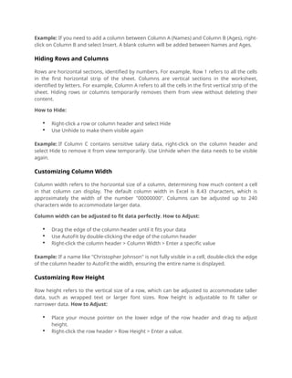
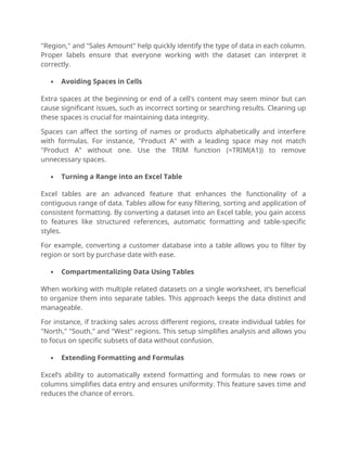
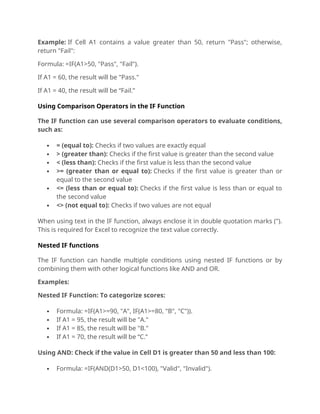
20. The RIGHT function is used to extract a specified number of characters from the
right end of a text string. This helps analyze structured data like IDs, codes, or file
extensions.
Syntax: =RIGHT(text, num_chars)
 Text: The string from which to extract characters
 num_chars: The number of characters to extract from the right
Use Case: Extract suffixes, codes, or other standardized endings in data.
 LEFT Function
The LEFT function extracts a specified number of characters from the left end of a
text string. This is often used to retrieve prefixes or other beginning parts of data.
Syntax: =LEFT(text, num_chars)
 Text: The string from which to extract characters
 num_chars: The number of characters to extract from the left
Use Case: Extract initials, prefixes, or standard codes from data.
 LEN Function
The LEN function calculates the number of characters in a text string, including
spaces and special characters. It is often used for data validation and analysis.
Syntax: =LEN(text)
 Text: The string whose length is to be determined
Use Case: Verify consistent lengths of codes, names, or ID numbers.
 SUBSTITUTE Function
The SUBSTITUTE function replaces specific text within a string with new text,
making it ideal for data cleaning or standardization tasks.
Syntax: =SUBSTITUTE(text, old_text, new_text, [instance_num])
 Text: The original text string
 old_text: The text to replace

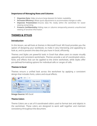
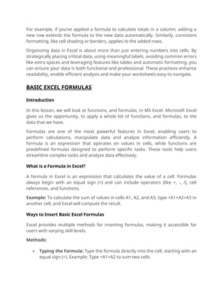
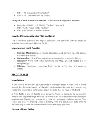
21.  new_text: The replacement text
 instance_num (optional): The occurrence of old_text to replace
Use Case: Standardize names, addresses, or other recurring text patterns.
 FIND Function
The FIND function locates the position of a specific substring within a string. It is
case-sensitive and helps identify parts of text for further manipulation.
Syntax: =FIND(find_text, within_text, [start_num])
 find_text: The substring to find
 within_text: The string to search in
 start_num (optional): The position to start the search
Use Case: Locate specific text or keywords in larger strings.
 CONCATENATE/CONCAT Function
The CONCATENATE (or CONCAT) function combines multiple text strings into one.
It is useful for creating full names, addresses, or customized labels.
Syntax: =CONCATENATE(text1, text2, ...) or =CONCAT(text1, text2, ...)
 text1, text2, ...: The strings to combine
Use Case: Merge first and last names, combine addresses, or create unique IDs.
 TRIM Function
The TRIM function removes extra spaces from a string, leaving only single spaces
between words. This is essential for cleaning up inconsistent data.
Syntax: =TRIM(text)
 Text: The string to clean
Use Case: Prepare messy datasets for analysis or presentation.
 PROPER Function

22. The PROPER function capitalizes the first letter of each word in a string while
converting the rest to lowercase.
Syntax: =PROPER(text)
 Text: The string to format
Use Case: Standardize name or title formats.
Importance of Text Functions
 Data Cleaning: Simplify text manipulation, such as removing unwanted
characters or standardizing formats.
 Efficiency: Automate repetitive tasks like extracting parts of strings or
replacing values.
 Analysis: Extract meaningful insights from text-based data, such as
identifying patterns or categorizing content.
 Flexibility: Combine text functions with other Excel features for more
advanced workflows.
CELL REFERENCES IN EXCEL
Introduction
In this lesson, we will look at cell referencing in MS Excel. Cell referencing is a very
important concept for all of you to understand, especially when we have to do any
kind of calculations with the data that's being provided in our Excel.
Cell references are the foundation of Excel formulas, allowing users to perform
calculations and manipulate data dynamically. A cell reference identifies a specific
cell or range of cells on a worksheet by combining a column letter and a row
number (e.g., "A1"). Excel supports three types of cell references—Relative,
Absolute, and Mixed—that provide flexibility and accuracy in calculations,
particularly when formulas are copied or moved across the worksheet.
How to Reference Cells in Excel
Cells in Excel are referenced by specifying their row number and column letter,
which together form the cell address. This system makes it easy to locate and use
data within the spreadsheet.

23. Example: The cell in Column B and Row 3 is referenced as "B3." You can use this
reference in a formula like =B3+10 to add 10 to the value in Cell B3.
This system allows for precise data manipulation and ensures that formulas can
dynamically adjust when applied to different locations.
Types of Cell References
Excel provides three types of cell references: Relative, Absolute, and Mixed. Each
type behaves differently when formulas are copied or moved, making them
essential for various tasks.
 Relative References: Adjust automatically when copied to new locations.
Ideal for calculations that need to adjust based on their position, such as
summing rows or columns.
 Absolute References: Remain fixed regardless of where the formula is
copied. Represented by a $ sign (e.g., $A$1). Useful when referring to a
constant value, such as a tax rate or a fixed reference cell.
 Mixed References: Combines relative and absolute references, fixing either
the row or the column. Helpful in scenarios requiring flexibility in one
direction (row or column) while maintaining a fixed reference in the other.
Advantages of Using the Correct Cell Reference
Using the correct type of cell reference can significantly enhance the efficiency and
accuracy of your calculations in Excel.
Practical Benefits
 Relative References: Automatically adjust for dynamic calculations
 Absolute References: Maintain consistency for constants or fixed values
 Mixed References: Provide flexibility in calculations that vary in one
direction but remain constant in the other
These references streamline repetitive tasks and minimize the risk of errors,
especially when working with large datasets or complex formulas.
Common Misunderstandings About Cell References
Misunderstandings about cell references can lead to calculation errors or
inefficient workflows.

24. Example of a Misunderstanding:
Believing that cell references use row letters instead of row numbers (e.g., thinking
"A1" is "Column A, Row A" instead of "Column A, Row 1"). Correct Understanding: A
cell reference like "C5" means Column C and Row 5.
Understanding the correct format ensures clarity and prevents mistakes in
formula creation and data management.
Importance of Cell References
 Flexibility: Enable dynamic adjustments to formulas when copied or moved
 Consistency: Allow fixed values to remain constant using absolute
references
 Efficiency: Save time by automating repetitive calculations
 Accuracy: Ensure correct results by using the appropriate reference type