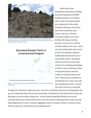
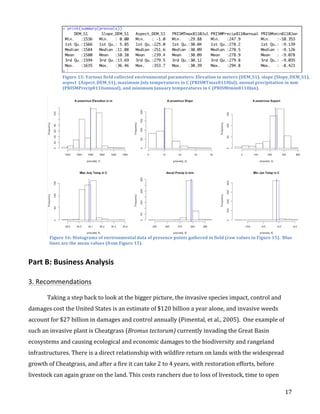
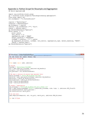
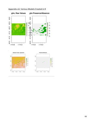
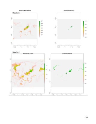
This document describes the creation of habitat distribution models for the endemic plant species Astragalis anserinus. The author collected environmental data for the species' range and used MaxEnt modeling in the R statistical programming language to create two habitat distribution models, MaxEnt1 and MaxEnt2. Both models were evaluated using metrics like AUC. A combination of the two models was used to make a final recommended habitat map. However, the author notes that some presence data points may be inaccurate and require field verification. An improved model incorporating verified data is recommended. The modeling provides a cost-effective way to predict habitat compared to solely using fieldwork.

1. 1
A.anserinus
Habitat
Modeling
Internship
Robert
Machol
University
of
Utah
Professional
Master
of
Science
and
Technology
In
conjunction
with:
Utah
Department
of
Agriculture
and
Food
March
2015

2. 2
Table
of
Contents:
Abstract…………………………………………………………………………………………………….3
Introduction………………………………………………………………………………………………4
Part
A:
Model
Development
1.
Methods……………………………………………………………………………………….6
2.
Results…………………………………………………………………………………………13
Part
B:
Business
Analysis
3.
Recommendations………………………………………………………………………17
Part
C:
Conclusion
and
Discussion
4.
Conclusion
&
Discussion……………………………………………………………..20
5.
Recommendations………………………………………………………………….…..23
Acknowledgements…………………………………………………………………………………24
References……………………………………………………………………………………………...25
Appendices
Appendix
i:
Soil
Data
Analysis…………………………………………………….…..26
Appendix
ii:
Raster
Data
Keys
…………………………………………………….…..29
Appendix
iii:
Batch
Attempts
Using
Model
Builder…………………………35
Appendix
iv:
Python
Script
for
Resample
and
Aggregation………….…..36
Appendix
v:
Models
Verified
in
Field
With
Corresponding
Points......37
Appendix
vi:
Field
Notes…………………………………………..……………………..39
Appendix
vii:
HyperNich
Model……………………………………………………….47
Appendix
viii:
Various
Models
Created
in
R……………………………………..48
Appendix
ix:
Sample
R
code…………………………………………………………….51
Appendix
x:
Colinearity
Analysis……………………………………………………..56
Appendix
xi:
Final
Map
and
Recommendation…………………………………57

3. 3
Abstract:
The
purpose
of
this
project
and
internship
with
Utah
Department
of
Agriculture
(UDAF)
was
to
create
a
Habitat
Distribution
Model
(HDM)
for
the
endemic
species
of
Astragalis
anserinus
(Goose
Creek
Milkvetch)
located
in
the
corner
of
Utah,
Idaho
and
Nevada
(Atwood,
Goodrich,
&
Welsh,
2011).
The
current
range
is
listed
by
the
U.S.
Fish
and
Wildlife
Services
(USFWS)
to
be
around
190
square
miles
(U.S.
Fish
and
Wildlife
Services,
2014).
Two
HDM
are
created
and
used
in
the
final
125
square
mile
area
(MaxEnt1
and
MaxEnt2),
while
the
recommended
habitat
area
is
207
square
miles.
The
HDM
were
created
using
the
Maximum
Entropy
(MaxEnt)
algorithm
(Hijmans
et
al,
2013).
Generally,
methods
were
to
collect
as
much
environmental
data
on
the
area
in
as
much
detail
as
possible,
with
a
goal
to
have
raster
data
at
3-­‐meter
resolution.
Course
data
utilized
bilinear
interpolation
and
was
made
“fuzzy”
to
better
fit
the
area
at
the
target
resolution.
After
aligning
the
data
using
ESRI
ArcMap
(commercial
GIS
application),
and
Python
(open
source
programming
language),
the
third-­‐party
Dismo
package
in
R
(a
statistical
analysis
language),
was
used
to
build
and
analyze
various
models
as
to
where
A.
anserinus
currently
grows.
The
Dismo
package
is
an
add-­‐on
program
specifically
made
to
model
species
distributions,
by
Robert
J.
Hijmans,
Steven
Phillips,
John
Leathwick
and
Jane
Elithas.
In
addition,
a
model
built
by
a
commercial
program,
HyperNiche,
was
used
for
verification
of
the
work
done
in
R.
During
the
course
of
the
internship,
my
mentor
at
UDAF,
Bracken
Davis,
and
I
added
a
mixture
of
about
700
presence
and
absence
points,
along
with
other
points
of
data
collected
by
USFWS,
to
have
a
total
of
about
1000
presence
and
absence
points
in
the
study
area.
Unfortunately,
many
of
the
presence
points
are
not
fully
confirmed,
as
Astragalis
anserinus
is
very
hard
to
differentiate?
Astragalis
utahensis
(Torr.).
In
fact,
without
seedpods
or
flowers
to
differentiate
the
two
species,
they
are
virtually
impossible
to
tell
a
small
specimen
apart.
Some
of
the
outlier
positive
presence
points,
I
believe,
are
questionable
and
more
likely
than
not,
there
are
false
positives
among
the
presence
points.
Verification
of
these
points
would
need
to
take
place
in
the
spring/early
summer
while
(and
if)
the
plant
is
flowering.
The
cost-­‐benefit
analysis
of
this
study
would
imply
that
creating
a
HDM
is
a
much
better
use
of
time,
compared
to
field
verification,
purely
for
the
reason
that
the
HDM
will
predict
where
a
plant
is
based
on
current
information.
However,
creating
a
model
is
easy,
running
and
interpreting
analytics
on
the
model
can
be
difficult.
Of
the
two
models
used
for
the
final
recommended
habitat,
the
MaxEnt2
model
was
simplified
so
that
the
analytics
were
run,
with
decent
results,
showing
an

4. 4
AUC
score
mean
of
72.6
(where
0.5
is
a
guess,
1.0
shows
all
true
positives).
MaxEnt1
model
was
too
large
to
run
the
analytics,
but
seems
the
better
model
from
a
user
point
of
view.
A
combination
of
the
two
models
was
created
to
better
represent
empirical
data,
and
a
third
model
is
highly
recommended
after
field
verification
of
both
the
model,
and
questionable
data
can
be
completed.
This
study
brings
up
many
questions
about
A.
anserinus,
and
shows
how
little
we
know
about
the
plant.
A
discussion
of
these
questions
is
of
the
opinion
of
the
author
alone,
but
is
not
without
relevance.
These
questions
include
whether
the
plant
is
particularly
tolerant
to
the
lack
of
soil
nutrients,
and
if
A.
anserinus
is
limited
in
range
by
anything
other
than
seed
dispersion.
Finally,
a
question
of
protecting
the
plant
might
do
the
plant
more
harm
than
good,
simply
by
stretching
the
resources
used
to
fight
invasive
species
in
order
to
comply
with
the
higher
cost
management
necessitated
by
the
Endangered
Species
Act.
Introduction:
The
modeling
the
distribution
of
species
is
becoming
an
increasingly
important
component
in
conservation
planning
(Pearson,
2007).
Conservation
planning
can
benefit
from
these
models
in
many
ways.
These
can
range
from
identifying
sites
and
borders,
understanding
the
social
and
ecological
impact
within
a
site,
identifying
threats
within
a
site,
and
helping
to
prioritize
resources,
to
name
a
few.
The
goal
of
this
project
was
to
create
a
Habitat
Distribution
Model
(HDM)
on
the
endemic
plant,
Astragalis
anserinus
(Goose
Creek
Milkvetch),
and
assess
the
possible
impact
in
which
the
HDM
might
have
on
the
conservation
planning.
Astragalis
anserinus
is
currently
being
considered
as
threatened
by
the
US
Fish
and
Wildlife
Service.
A.
anserinus
has
only
been
found
an
area
of
approximately
17
square
acres
in
Utah,
with
a
total
range
that
is
approximately
190
square
miles
in
Nevada,
Idaho,
and
Utah
in
and
around
the
Goose
Creek
Drainage
(Figure
1).
The
Goose
Creek
Drainage
is
recognized
as
an
area
to
preserve
by
some
wilderness
conservation
groups,
and
is
listed
as
an
area
to
be
considered
for
protection
within
the
National
Wilderness
Preservation
Program.
The
Biodiversity
found
within
the
Goose
Creek
Drainage
is
unique
because
it
is
grassland
with
gentle
topography
and
a
transition
zone
between
the
Great
Basin
and
Snake
River
Plain
(Lukez,
2011).
In
2004,
a
petition
for
the
endemic
species
was
given
to
the
U.S.
Fish
and
Wildlife
to
put
A.
anserinus
under
the
protection
of
the
Endangered
Species
Act,
and
this
decision
is
assumed
to
occur
by
2016
(U.S. Fish and Wildlife
Service, 2014).

5. 5
Figure
1:
Range
for
A.
anserinus
(US
FWS,
2014),
calculated
at
~190
sq.
miles
In
2007,
there
was
significant
damage
to
the
population
of
A.
anserinus
due
to
wildfires.
Before
2007,
there
was
an
estimated
population
of
60,000.
There
is
a
direct
correlation
of
wildfire
return
and
invasive
weeds
within
the
habitat
area
of
native
plant
species
on
the
Great
Plains
(Tilley,
St.
John
and
Ogle,
2011).
The
habitat
has
also
changed
significantly
with
the
intentional
seeding
of
crested
wheatgrass
(Agropyron
cristatum),
a
commonly
planted
species
to
establish
grazing
lands
(Tilley,
St.
John
and
Ogle,
2011).
Although
there
is
no
direct
habitat
competition
from
crested
wheatgrass,
due
to
Goose
Creek
Milkvetch’s
primary
habitat
of
fine,
volcanic
detritus
and
the
tendency
to
grow
on
steeper
slopes,
it
has
been
shown
that
the
presence
of
crested
wheatgrass
leads
to
a
generally
diminished
biodiversity
(Ogle,
2006).
This
project
was
under
the
supervision
of
Bracken
Davis,
an
Environmental
Scientist
at
the
Utah
Department
of
Agriculture
and
Food
(UDAF).
The
Utah
Legislature
created
UDAF
in
1921
by
consolidating
various
agencies
with
the
State
Board
of
Horticulture,
which
was
founded
in
1896,
all
to
promote
Utah
agriculture.
Focused
on
the
healthy
growth
of
Utah’s
agriculture
and
protecting
Utah’s
natural
resources,
UDAF
helps
draft
legislation
to
meet
the
challenges
of
urban
sprawl,
preserving
open
lands
and
protecting
the
environment
while
working
with
farmers,
ranchers
and
community
leaders
to
protect
farmlands.
UDAF
has
many
responsibilities,
divisions
and
programs
under
its
umbrella,
including
the
Animal
Industry,
Plant
Industry
and
Conservation,

6. 6
Food
Regulatory
Services,
Marketing
and
Economic
Development,
Conservation
Commission,
Homeland
Security,
Laboratory
Services,
Administrative
Services,
and
Communications
and
Public
Information.
“The
Department
of
Agriculture
and
Food
is
responsible
for
the
administration
of
Utah's
agricultural
laws,
which
mandate
a
wide
variety
of
activities
including
inspection,
regulation,
information,
rulemaking,
loan
issuance,
marketing
and
development,
pest
and
disease
control,
improving
the
economic
position
of
agriculture,
and
consumer
protection”
(Utah
Department
of
Agriculture,
2014).
It
is,
therefore,
part
of
UDAF’s
responsibility
to
make
sure
that
Utah’s
lands
are
managed
in
a
manner
that
conserves
all
species,
including
A.
anserinus,
where
possible.
Part
A:
Model
Development
1.
Methods
This
project
began
with
the
collection
of
various
environmental
data
pertaining
to
the
study
area.
The
study
area
chosen
gave
a
wide
berth
of
the
known
habitat
of
A.
ansernius,
in
the
hopes
of
finding
the
plant
well
outside
of
the
known
range.
The
overall
study
area
was
approximately
100
miles
in
both
length
and
width,
giving
an
approximate
1000
square
mile
study
area
(Figure
2).
This
was
an
unintentional
result
in
the
fact
that
the
known
range
ran
in
a
diagonal
and
it
was
an
attempt
to
give
the
corners
a
wide
breadth.
The
project
was
conducted
using
the
spatial
reference
of
WSG1984,
with
the
study
area
extent
of
about
42.5
to
41.2
North
latitude,
-­‐
114.9
to
-­‐113.5
West
longitude.
There
were
171
rasters
collected
and
analyzed
in
the
models
built,
including
Land
Cover
and
Soil
data
from
National
Resource
Conservation
Service
(USDA),
digital
elevation
models
(DEM)
and
Orthoimagery
from
USGS,
Climate
data
from
PRISM
(see
Appendix
i).
Other
layers
were
created
by
need.
The
Integrated
Moisture
Index
(IMI)
was
created
using
the
DEM
layer.
This
method
is
a
close
approximation
to
actual
water
accumulation
(Iverson
et.al.,
Figure
2:
Project
Study
Area
(~1000
sq.
miles)
with
the
current
range
in
white
(~190
sq.
miles)
Figure
3:
Equation
used
in
Raster
Calculator
to
create
the
IMI
layer:

7. 7
1997,
Figure
3).
Solar
energy
was
also
created
off
of
the
DEM
in
ArcMap,
a
process
that
took
10
days
to
run
for
the
given
study
area.
The
results
given
were
a
calculation
of
the
average
watt-­‐hours
per
square
meter
for
the
entire
year.
Any
categorical
data
was
separated
into
its
own
individual
raster
layer
and
given
a
score
of
0
or
1
(absence
or
presence),
and
then
given
fuzzy
values
decreasing
over
9
meters
(3
cells).
The
landcover
data
and
the
geology
data
necessitated
a
mosaic
function
to
combine
multiple
areas
together,
and
then
the
data
layer
names
had
to
be
aligned
and
changed
as
the
various
data
had
the
annoying
habit
of
changing
names
as
it
crossed
state
boundaries
(Figure
4).
The
landscape
raster
has
a
key
(Appendix
ii),
but
was
never
utilized
in
any
of
the
final
models,
as
they
never
scored
high
on
any
of
the
various
tests.
Data
for
various
soil
layers
is
continuous
measurement
of
various
levels
of
soil
types.
The
soil
layers
came
separately
by
state,
and
since
the
study
area
encompasses
three
states
this
also
proved
to
be
problematic.
First,
the
soil
layers
had
to
be
joined
together
(using
the
mosaic
function),
and
then
clipped
to
the
study
area
before
each
soil
layer
was
separated
into
its
own
raster.
The
soil
layers
were
separated
by
values
and
analyzed
as
their
own
individual
raster
layer
(Soil
key
in
Appendix
ii).
All
raster
data
was
either
at
3-­‐meter
resolution,
or
was
re-­‐sampled
to
3-­‐meter
resolution,
either
using
bilinear
interpolation
or
aggregated
an
averaging
depending
if
the
raster
was
lower
or
higher
resolution
(Figure
5).
Figure
4:
Clear
changes
in
soil
type
data
across
state
boundaries
prove
problematic.
Figure
5:
Bilinear
Interpolation
method
used
on
a
5km
resolution
PRISM
raster,
reduced
to
3m
resolutions.

8. 8
Much
of
the
raster
manipulation
took
place
in
ArcMap,
but
the
development
of
all
HDM
building
took
place
in
R,
which
is
where
a
Non-­‐Coincident
problem
was
recognized.
For
the
model
building
to
take
place,
each
raster
had
to
have
exactly
the
same
columns
and
rows.
The
Non-­‐
Coincident
problem
occurred
in
ArcMap
with
a
bug
in
the
Clip
function;
an
extra
row
or
column
would
be
added
to
the
raster.
At
the
size
and
resolution
the
rasters
were
in,
this
was
evidently
a
bug
with
ArcMap
that
did
not
tend
to
occur
with
smaller
rasters.
Among
the
solutions
tried
was
a
homemade
version
of
re-­‐sampling
and
clipping
in
which
a
raster
would
have
values
averaged
into
points,
based
on
number
of
required
columns
and
rows.
These
points
would
then
be
turned
back
into
a
raster,
now
with
the
averaged
given
value.
In
small
test
rasters,
this
was
a
successful
strategy,
but
would
fail
in
large-­‐scale
runs.
Of
course,
it
would
be
a
few
days
of
running
before
the
process
would
come
back
with
an
error.
Eventually,
an
alternative
to
the
Clip
function,
Extract
By
Rectangle,
ran
successfully
at
large
scale.
Various
models
using
Model
Builder
was
used
to
automate
this
process,
which
would
work
in
test
runs
but
they
would
again
fail
in
large
scale
and
batch
(Appendix
iii).
Later,
I
needed
to
aggregate
rasters
to
a
larger,
30
meter,
resolution,
when
Python
scripts
were
utilized
with
success
(Appendix
iv).
Figure
7:
Random
points
generated
within
survey
sites
in
unrepresented
population.
Figure
6:
While
not
all
of
the
areas
within
survey
sites
are
this
densely
populated,
many
are.
Random
points
were
generated
within
survey
areas
to
help
generate
baseline
data.

9. 9
During
this
project,
both
point
and
polygon
data
were
obtained
from
US
Fish
and
Wild
Life
Services.
While
some
point
data
were
previously
collected,
much
of
the
point
data
were
outside
of
polygon
survey
sites.
These
survey
sites
where
known
populations
of
A.
anserinus
species.
For
this
study,
random
points
were
generated
within
the
survey
polygons.
While
this
is
not
the
best
situation
(real
data
is
better
than
pseudo
data),
given
the
limited
time
and
resources,
and
taking
into
account
the
size
of
the
study
area,
this
technique
helped
to
get
baseline
environmental
data
from
rasters
(elevation,
temperature,
etc.)
in
the
modeling
program.
It
is
within
these
polygons
that
A.
anserinus
grows
in
fairly
dense
populations
(Figure
6),
and
by
creating
random
points
within
the
polygons,
the
model
will
have
the
assigned
environmental
data
from
these
known
areas
without
the
need
to
visit
these
sights.
Within
each
survey
site,
up
to
three
random
points
were
collected,
spaced
by
at
least
a
quarter
mile.
This
limited
some
smaller
survey
sites
to
only
one
or
two
random
points,
while
larger
sites
were
given
a
maximum
of
three
points
to
capture
the
general
environmental
values
of
the
give
polygons
without
overwhelming
the
model
with
a
huge
amount
of
unverified
points
(Figure
7).
A
half-­‐mile
buffer
around
the
polygons
was
created
to
capture
some
of
the
absence
data.
Ideally,
in
the
future,
the
polygon
sites
can
have
verified
point
data
assigned
by
field
observations
for
further
modeling
endeavors
such
as
this
one.
In
all,
total
of
787
presence
points
and
362
absence
points
were
used
in
this
HDM
(Figure
8),
with
190
presence
points,
and
108
absence
points
randomly
created
from
these
polygons.
There
was
a
huge
amount
of
data
analyzed
during
this
project.
By
the
end
there
were
171
rasters,
all
at
3-­‐meter
resolution.
Of
the
171
rasters
analyzed,
there
was
a
select
final
six,
which
were
used
only
in
the
MaxEnt2
model,
and
then
in
the
combined
(MaxEnt1
and
MaxEnt2)
final
model
(discussed
below).
However,
before
the
final
model,
there
were
a
large
variety
of
models
created
for
analysis
and
verification
purposes,
using
a
range
of
raster
data
and
techniques.
Figure
8:
Plotted
in
R;
total
presence
and
absence
points
in
HDM

10. 10
Compiling
and
sorting
through
the
171
rasters
through
various
means,
with
commonsense
prioritizing,
cut
the
171
rasters
to
six
final
rasters
(Appendix
i).
How
significant
raster
data
is
to
the
various
models
can
change
depending
on
how
you
analyze
the
data.
For
example,
fitting
data
to
a
linear
model
will
give
you
different
error
report
than
a
curved
model.
Included
in
the
analysis
of
relevant
data,
rasters
were
“fit”
to
a
variety
of
models
and
then
analysis
of
those
rasters
would
be
conducted
(Figure
9).
For
this
exercise,
there
was
a
variety
of
models
that
the
data
was
fit
to,
and
thus
a
variety
of
relevant
values
that
were
given
for
each
raster
and
compiled
into
a
document
for
analysis
(Appendix
i).
For
the
171
rasters,
the
following
values
were
considered
before
selecting
the
final
six
rasters
for
the
last
analysis:
Coefficients
(p-­‐Values),
Anova
Figure
9:
Example
of
obtaining
p-­‐value
(this
case
z-­‐value)
of
a
series
of
rasters
using
a
GLM.
These
values
would
change
depending
on
data
points,
raster’s,
and
type
of
model
used
to
analyze.
Final
analysis
available
in
Appendix
i
Figure
10:
Final
6
raster
layers
selected
for
final
model
(MaxEnt2).
A
direct
comparable
AIC
score
to
MaxEnt1
was
not
available
due
to
the
changing
nature
of
the
project.
This
was
used
to
obtain
p-­‐values
for
the
raster
data
layers.

11. 11
(F-­‐test),
Drop1
(F-­‐test),
boosted
Regression
Tree,
and
a
self-­‐created
biased
variable
“BioClimate”,
were
used
to
simplify
the
model
and
cut
rasters
to
the
final
six
selected
in
the
last
MaxEnt2
model.
For
the
BioClimate
values,
there
is
an
explanation
in
Appendix
i
for
each
raster
layer
as
to
why
the
given
value
was
assigned
to
some
raster
layers
and
not
others.
The
reason
for
the
BioClimate
values
was
for
the
sake
of
common
sense.
For
example,
certain
rasters
would
score
high
on
co-­‐
efficiency
tests
(p-­‐values)
that
would
not
make
sense,
such
as
minimum
July
temperatures.
This
would
fit
the
models
well
because
they
have
very
little
variation,
but
really
do
not
have
much
to
do
with
the
actually
plant
growth;
correlation
is
not
necessarily
causation.
Other
rasters
would
not
have
as
high
a
score,
however
it
was
deemed
important
to
include
them,
for
example
to
capture
Goose
Creek
Milkvetch’s
minimum
and
maximum
temperature
tolerance.
A
prioritizing
system
was
used
in
the
compiled
raster
score
document
(Appendix
i)
to
go
through
all
171
rasters
and
select
the
final
six
rasters
that
would
be
included
in
a
final
analysis
(Figure
10)
and
predictive
model
(MaxEnt2,
discussed
below).
Of
the
many
predictive
models
created,
two
distribution
models
were
used
for
field
verification;
first
a
HyperNiche
model,
then
a
Maximum
Entropy
(MaxEnt)
model
(Appendix
v).
The
HyperNiche
model
utilizes
a
program
by
the
same
name,
which
is
made
for
professionals
creating
HDM,
and
must
be
purchased
to
use.
This
program
is
a
“black
box”
program,
which
has
protected
code.
Part
of
the
purpose
of
the
internship
at
UDAF
was
to
code
for
my
own
models,
which
is
why
there
were
so
many
models
created
during
this
project.
UDAF
had
the
HyperNiche
program
on
site,
and
it
was
used
for
verification
purposes.
The
HyperNiche
model
was
created
first
while
programming
continued
in
R
(Appendix
vii).
The
second
model
used
in
the
field
was
the
MaxEnt
model
(MaxEnt1).
The
MaxEnt1
model
was
selected
for
field
verification
for
a
few
reasons;
the
popularity
of
the
MaxEnt
model
technique
(MaxEnt
process
generally
discussed
below),
the
quickly
disappearing
summer
season,
and
that
the
MaxEnt1
predictive
model
fit
very
closely
to
the
HyperNiche
model
that
gave
confidence
that
it
was
the
model
with
which
to
start
with.
Fieldwork
was
conducted
for
verification
of
models
as
well
as
the
collection
of
additional
point
data.
Over
700
additional
absence
and
presence
points
were
collected
from
various
field
excursions,
both
in
and
out
of
survey
sites.
A
presence
point
was
identified
by
walking
10
meters
in
each
of
the
cardinal
directions
from
the
flagged
point,
and
either
deemed
as
a
positive
or
negative
point
depending
if
there
was
a
plant
viewed
within
that
range.
Both
the
HyperNiche
model
and
the
MaxEnt1
model
had
field
verification
work
done
that
lasted
a
couple
of
weeks
each.
With
help
from
Bracken
Davis
and
UDAF,
there
were
about
200
man-­‐hours
spent
in
the
field,

12. 12
approximately
half
the
time
on
each
predictive
model
(HyperNiche
and
MaxEnt1),
and
field
notes
were
collected
during
verification
(Appendix
vi).
A
final
model
was
created
using
Maximum
Entropy
(MaxEnt1
and
MaxEnt2
in
Appendix
vii)
and
an
error
report
was
created
for
MaxEnt2
(error
report
in
Results
section
below).
Example
coding
used
in
R
for
the
MaxEnt
model,
along
with
raster
and
point
analysis
is
available
in
the
Appendix
section
(Appendix
ix).
The
MaxEnt2
model
has
a
new
area
in
the
Northeast
section
of
the
study
area
that
is
showing
positive
results,
but
at
this
time
has
not
yet
been
surveyed
nor
field
verified.
This
model
has
not
been
field
verified
because
of
the
ending
of
the
summer/fall
season,
as
well
as
the
ending
of
the
UDAF
internship.
In
the
beginning,
it
was
not
predetermined
that
the
MaxEnt
program
was
to
be
selected
as
a
final
modeling
technique,
but
rather
through
analyzing
and
experimenting
with
a
variety
of
modeling
techniques
that
the
MaxEnt
method
was
selected
for
this
study.
The
creation
of
many
predictive
models
were
created
and
analyzed
in
R
(Appendix
viii)
before
and
after
the
first
MaxEnt
model,
and
in
the
end
the
MaxEnt
models
were
selected
as
the
final
HDM.
Many
of
the
models
created
had
almost
no
positive
area,
or
extremely
limited
area
determined
to
be
A.
anserinus
habitat.
The
first
MaxEnt
model
(MaxEnt1)
not
only
looked
good,
but
it
fit
the
area
which
was
previously
known
to
be
A.
anserinus
habitat,
and
had
positive
areas
that
matched
the
HyperNiche
model
as
well.
This
was
encouraging,
because
the
two
models
utilized
different
combinations
of
raster
data
to
create
similar
predictive
maps
(Appendix
v).
After
determining
that
MaxEnt
fit
the
study
area
well,
it
was
utilized
for
field
verification
and
then
determined
as
the
primary
model
for
the
remainder
of
the
study.
MaxEnt
has
been
identified
by
many
studies
to
be
a
highly
competitive
method
(Beane,
et
al,
2013).
The
MaxEnt
modeling
technique
itself
is
a
robust
modeling
method,
utilizing
a
presences-­‐only
input
technique
to
build
models.
The
MaxEnt
output
is
created
from
probability
distributions
from
incomplete
information
to
produce
probabilities
from
zero
to
one.
The
presence-­‐only
MaxEnt
takes
a
list
of
location
inputs,
along
with
given
environmental
data
(i.e.,
temperature,
elevation,
etc.)
across
the
study
area
by
cells.
MaxEnt
then
takes
a
sample
of
background
locations
that
is
compared
against
the
presence
locations.
The
environmental
data
at
the
presence
locations,
as
well
as
the
background
locations,
are
taken
into
account
when
creating
the
output.
The
negative
data
(or
absence
points),
which
is
always
suspect
because
there
is
no
way
to
know
if
the
plant
wont
grow
at
a
location
(just
that
it
is
currently
not
there),
is
not
required
in
the
creation
of
the
model.
The
negative
data
is
used
for
testing
purposes,
and
the
model
can
use
both
categorical
and
continuous
data
(Beane,
et
al,
2013).
There
are
a
multitude
of
settings
and
interpretations
of
MaxEnt
modeling
technique
itself,
which
go
beyond
the
scope
of
this
study.

13. 13
Entire
papers
have
been
written
on
the
various
techniques
that
can
be
utilized
for
MaxEnt
alone
(Merow,
et.al.,
2013),
but
for
this
study
the
default
settings
were
used
or
otherwise
specified
by
the
document
by
Hijmans
&
Elith,
Species
distribution
modeling
with
r
(2013).
Discussed
below
are
the
implementations
and
considerations
taken
for
Spatial
Bias
within
the
MaxEnt
modeling.
The
program
for
Maximum
Entropy
is
a
third
party
package
that
was
freely
downloaded
and
incorporated
into
R
as
a
machine-­‐learning
program
(Hijmans
&
Elith,
2013).
2.
Results
The
final
six
raster
layers
were
selected
as
DEM
(Digital
Elevation
Map),
solar
energy,
IMI,
maximum
July
temperature
(1981-­‐2010),
minimum
February
temperature
(1981-­‐2010),
and
June
precipitation
(1971-­‐2000)
(Figure
11).
The
colinearity
analysis
conducted
showed
nothing
surprising
between
raster
layers
(Appendix
x).
Further
analysis
shows
all
layers
have
highly
significant
p-­‐value
(Figure
10),
indicating
the
rasters
are
relevant
with
a
confidence
of
95%
or
better.
There
were
two
ways
that
the
various
models
are
compared:
AIC
(Akaike
information
criterion)
and
AUC
(Area
Under
the
Curve).
The
AIC
score
is
a
comparative
score
in
which
to
compare
the
goodness
of
fit
to
the
complexity
of
a
model;
the
lower
the
score
the
better
the
model.
However,
the
AIC
score
does
not
give
any
indication
as
to
the
quality
of
the
model
itself,
instead
the
AIC
score
will
tell
the
user
as
to
how
well
the
data
fits
the
model.
This
is
a
good
way
to
compare
one
model
to
another
model,
so
long
as
all
the
data
is
identical
with
few
parameters
(Beane
et.
al.,
2013).
To
help
further
simplify
the
model
for
analysis
purposes
these
raster
layers’
resolution
was
lowered
from
3-­‐meter
to
30-­‐meter
resolution
(thus
lowering
the
amount
of
data
for
the
predictive
model)
by
aggregating
using
Python
script
that
averaged
the
area
(Appendix
iv).
The
final
model
(MaxEnt2)
AIC
score
is
fairly
high,
higher
than
some
of
the
other
models
built,
but
this
was
acceptable
as
simplifying
the
model
was
the
ultimate
goal
in
this
step.
The
AIC
score
for
MaxEnt2
was
not
compared
to
other
models
utilizing
both
the
final
six
raster
layers,
nor
the
final
point
data,
thus
making
this
AIC
score
obsolete
at
the
moment,
but
could
be
used
in
the
future
comparing
other
models
using
the
current
set
of
data.
It
was
because
of
the
very
nature
of
this
project,
with
a
continual
influx
of
raster
data
and
point
data,
that
the
AIC
analysis
was
not
a
good
choice
of
analysis,
as
all
AIC
scores
must
have
few

14. 14
parameters
and
have
identical
data
between
models
(Beane
et.
al.,
2013).
For
this
reasons,
this
project
focused
overall
HDM
analysis
using
the
AUC
score.
The
AUC
score,
also
sometimes
referred
to
as
Area
Under
the
ROC
(Receiver
Operating
Characteristic)
Curve
(Figure
13),
is
generated
by
plotting
the
true
positive
rate
against
the
false
positive
rate
to
give
a
graphical
plot
(Tape,
2014).
The
AUC
score
ranges
from
0
to
1,
where
0.5
is
as
good
as
a
guess
and
a
high
score
of
1.0.
By
the
time
a
predictive
model
would
be
finished
being
created
(which
sometimes
took
days),
very
often
there
would
be
additional
data
of
some
sort
and
the
evaluation
process
would
start
all
over
again.
Figure
11:
Values
of
DEM,
Solar
Energy,
IMI,
Max
July
Temp,
Minimum
February
Temp,
June
Precipitation
Figure
12:
Final
model
merged
two
Maximum
Entropy
models
to
better
represent
empirical
data.
The
dark
green
is
MaxEnt1,
light
green
is
MaxEnt2.
See
Appendix
xi
for
final
model
and
map.

15. 15
When
using
the
AUC
scores,
predictive
models
can
be
spatially
biased;
the
larger
the
area
in
which
the
model
encompasses,
the
higher
the
AUC
score
will
be
(Hijmans
&
Elith,
2013).
Within
the
Dismo
package
is
a
function
designed
to
evaluate
the
spatial
bias,
labeled
in
Dismo
as
the
Spatial
Sorting
Biased
function
(SSB).
The
SSB
function
gives
the
difference
between
two
point
data
sets
in
the
average
distance
to
the
nearest
point
in
a
reference
dataset
(Hijmans
&
Elith,
2013).
The
SSB
evaluation
can
be
used
to
remove
the
spatial
biased
from
the
AUC
score
(see
Appendix
xi
for
code
example
set
in
R).
The
AUC
score,
with
the
spatial
biased
removed
using
the
SSB
function
in
R
with
the
Dismo
package
(Hijmans
&
Elith,
2013),
was
used
to
analyze
the
error
of
the
final
predictive
MaxEnt2
model
(Appendix
xi).
Because
the
AUC
uses
a
sample
of
presence
points
to
train
and
test
the
model,
one
AUC
score
of
a
model
will
have
a
different
score
than
another
AUC
score
depending
on
which
points
were
randomly
selected
as
train/test
data.
An
example
of
one
such
iteration
shows
the
AUC
score
(with
SSB
removed)
at
0.746
(Figure
13).
The
final
MaxEnt2
AUC
score
averages
100
of
such
individual
models,
with
random
train/test
points
on
each,
with
mean
AUC
of
Figure
13:
AUC
score
with
true
positive
to
false
positive
rate.
Figure
14:
Histogram
of
AUC
scores
built
from
100
models,
each
with
random
train/test
data.
A
score
of
0.5
is
considered
a
guess,
with
a
high
score
of
1.

16. 16
0.72
and
along
with
an
accompanied
histogram
of
all
the
100
iterations
run
(Figure
14).
A
mean
AUC
score
of
0.72
was
about
as
good
as
any
model
created
during
this
project;
there
was
never
a
single
AUC
score
that
was
recorded
over
a
0.76
on
any
model
created,
with
the
SSB
removed
(with
many
much
worse,
some
even
below
0.5!).
The
field
data
gathered
shares
much
of
the
already
recorded
information
given
on
A.
anserinus
from
the
Goose
Creek
Milkvetch
Plant
Guide
by
Atwood,
Goodrich
and
Welsh.
The
following
is
a
summary
of
environmental
values
of
A.
anserinus
from
the
presence
points
gathered
in
the
field
(Figure
15
&
16
–
Note
that
the
randomly
created
points
from
polygon
data
gathered
from
the
U.S.
Fish
and
Wildlife
Services
are
not
taken
into
consideration
for
the
following
information).
For
example,
Atwood
Goodrich
and
Welsh
place
the
plant
from
1,500
to
1,790m
in
elevation,
while
the
field
data
collected
gives
elevation
values
between
1,539
and
1,635
meters.
Certainly
the
field
points
are
incomplete
but
this
project
adds
some
insight
as
to
where
to
find
the
plant
in
the
field.
According
to
the
mean
environmental
data,
the
plant
tolerates
temperatures
well
bellow
freezing
in
winter
of
-­‐9
oC,
annual
precipitation
of
278.9
mm
(rain
plus
snowmelt),
maximum
July
temperatures
of
30.09
oC,
mostly
(based
on
quarterly
data)
found
on
slopes
from
about
6
to
14
degrees,
and
an
aspect
mostly
(based
on
quarterly
data)
ranging
from
South
West
(225o)
to
West
(279o)
facing
slopes.
Of
particular
interest
on
these
six
parameters
listed
is
the
annual
precipitation,
indicating
that
there
might
be
a
fairly
narrow
range
in
which
the
plant
may
grow.
While
elevation
has
always
been
a
good
indication
as
to
where
this
plant
can
be
found,
I
feel
it
is
more
of
a
consequence
of
the
combined
limits
of
range
in
which
the
plant
is
found
and
dispersal
methods.
As
mentioned
above,
there
seems
to
be
a
lack
of
soil
data
that
captures
the
plants
obvious
preference
for
the
Salt
Lake
Formation.
During
this
study,
one
technique
that
was
used
(but
not
in
the
final
results)
was
to
try
and
capture
the
preference
for
the
lighter
colored
Salt
Lake
Formation
soil
by
utilizing
and
analyzing
the
Orthoimagery,
with
the
blue
band
having
shown
up
as
a
significant
predictive
variable
multiple
times
by
multiple
models,
and
may
have
a
significant
roll
in
the
future
of
determining
the
habitat
for
A.
anserinus.
The
final
recommended
HDM
from
this
paper,
also
discussed
in
the
recommendation
section
below,
was
a
combination
of
the
two
MaxEnt
models,
MaxEnt1
and
MaxEnt2.
Each
of
these
models
covered
a
part
of
the
range
and
presence
of
A.
anserinus
that
better
encompassed
the
extent
of
the
species,
while
the
majority
of
the
two
models
still
overlapped
(Figure
12).
The
final
recommended
distribution
map
is
given
a
quarter
mile
buffer
to
help
fill
in
gaps
and
give
a
small
boarder
zone
around
the
given
MaxEnt
models.
(See
Appendix
xi
for
the
final
map
and
recommendations).

17. 17
Part
B:
Business
Analysis
3.
Recommendations
Taking
a
step
back
to
look
at
the
bigger
picture,
the
invasive
species
impact,
control
and
damages
cost
the
United
States
is
an
estimate
of
$120
billion
a
year
alone,
and
invasive
weeds
account
for
$27
billion
in
damages
and
control
annually
(Pimental,
et
al.,
2005).
One
example
of
such
an
invasive
plant
is
Cheatgrass
(Bromus
tectorum)
currently
invading
the
Great
Basin
ecosystems
and
causing
ecological
and
economic
damages
to
the
biodiversity
and
rangeland
infrastructures.
There
is
a
direct
relationship
with
wildfire
return
on
lands
with
the
widespread
growth
of
Cheatgrass,
and
after
a
fire
it
can
take
2
to
4
years,
with
restoration
efforts,
before
livestock
can
again
graze
on
the
land.
This
costs
ranchers
due
to
loss
of
livestock,
time
to
open
Figure
15:
Various
field
collected
environmental
parameters:
Elevation
in
meters
(DEM_S1),
slope
(Slope_DEM_S1),
aspect
(Aspect_DEM_S1),
maximum
July
temperatures
in
C
(PRISMTmax8110Jul),
annual
precipitation
in
mm
(PRISMPrecip8110annual),
and
minimum
January
temperatures
in
C
(PRISMtmin8110Jan).
Figure
16:
Histograms
of
environmental
data
of
presence
points
gathered
in
field
(raw
values
in
Figure
15).
Blue
lines
are
the
mean
values
(from
Figure
15).

18. 18
lands
up
for
grazing
again,
and
restoration
costs.
Areas
that
are
in
a
degraded
state
have
a
tendency
to
stay
that
way
unless
serious
restoration
efforts
take
place,
and
even
then
it
can
take
upwards
of
a
century
to
restore
to
healthy
conditions,
if
they
can
be
restored
at
all.
Prevention
is
key
with
a
healthy
sagebrush
rangeland
(which
our
Astragalis
anserinus
is
found),
costing
~$20/acre
per
year
for
treatment
with
100%
effective
rate.
With
ecological
degradation
due
to
overuse
and
noxious
weed
invasion,
costs
and
time
for
restoration
projects
skyrocket
and
methods
are
not
nearly
as
effective.
Wildfire
rates
and
cost
per
acre
rates
increase
by
a
factor
of
10,
and
pre-­‐fire
control
work
is
much
more
effective
than
post-­‐fire
restoration
efforts
(Kobayashi
et
al.,
2010).
With
this
in
mind,
we
turn
our
attention
back
to
the
Astragalis
anserinus
habitat.
Continued
control
work
is
crucial
for
maintaining
high
biodiversity
and
ecological
resilience
in
the
face
of
invasive
species,
such
as
the
Cheatgrass
example
above.
If
and
when
A.
anserinus
is
officially
on
the
Threatened
and
Endangered
List,
UDAF
will
have
to
change
certain
types
of
control
work,
for
example
how
it
sprays
chemical
agents
in
the
area,
which
would
be
limited
due
to
state
and
federal
guidelines
in
an
area
with
a
protested
species
(Environmental
Assessment,
2002).
This
HDM
could
help
agencies
by
focusing
the
A.
anserinus
range
down
to
a
smaller
area,
the
survey
work
needed
will
hopefully
be
significantly
narrowed,
saving
time
and
money.
Currently,
the
suggested
habitat
range
from
the
USFWS
is
approximately
190
square
miles.
The
final
model
created
had
an
area
of
125
square
miles,
a
decrease
in
area
of
65.8%.
However,
because
the
final
model
is
fragmented
with
large
gaps
between
areas,
the
final
recommended
area
(Appendix
xi)
has
an
area
of
about
207
square
miles,
about
a
9%
increase
of
size.
While
this
will
increase
the
management
and
invasive
control
costs
of
the
overall
habitat
area,
there
is
a
difference
of
about
85
square
miles
that
the
current
range
and
the
recommended
range
do
not
align
(which
is
about
45%
of
the
total
recommended
207
square
mile
range),
which
would
save
a
tremendous
amount
in
funding
fieldwork
to
find
the
this
difference
in
range
by
field
work
alone.
Let’s
focus
on
a
more
comprehensive
cost/benefit
analysis
of
comparing
a
HDM
to
a
pure
fieldwork
approach
to
a
computer
modeling
approach.
A
fieldwork
approach
to
finding
the
habitat
would
involve
walking
transects
across
the
land
to
find
the
plant.
A
square
acre
is
208.71
feet
squared,
which
we
will
round
down
to
200
square
feet
for
the
ease
of
this
calculation.
The
fieldwork
that
I
was
a
part
of,
we
were
walking
transects
which
was
about
10
to
20
feet
apart,
lets
say
for
this
comparison
20
feet
apart.
Bracken
Davis
suggested
that
this
transect
could
be
as
far
apart
as
50
feet
apart;
let’s
look
at
both
to
look
at
maximum
and
minimum
costs.
Walking
one
square
acre
(200
ft)
of
transecting
20
feet
apart
(200
ft2
acre
at
20
foot
transects
apart
=
10
transects/acre),
gives
10
transects
*
200ft
=
2000
ft/square
acre.
At
50
feet
per
transect,
it
would

19. 19
be
4
transects
*
200ft
=
800
ft/
square
acre.
Walking
at
1
mile/hour
is
equivalent
to
walking
5280
feet
per
hour,
so
walking
800
to
2000
feet
per
square
acre
is
the
equivalent
of
0.15
to
0.38
hour
per
acre.
Now,
calculate
the
per
hour
cost
of
the
employee
to
figure
out
the
dollar
per
acre
costs.
For
simplicity’s
sake,
let’s
use
a
field
workers
pay
rate
of
around
$15/hour
(This
could
range
from
$10/
hour
to
over
$30/hour,
depending
on
who
is
doing
the
work).
This
could
then
range
from
0.15
hour/acre
*
$15/hour
=
$2.25/hour
to
0.38
hour/acre
*
$15/hour
=
$5.7/hour,
depending
on
how
you
space
out
the
transects.
(Note:
On
the
higher
end
of
this
would
be
an
employee
making
$30
per
hour,
walking
transects
at
10
feet
apart,
maxing
the
field-­‐work
cost
of
upwards
of
$22.8/hour!)
Let’s
suppose
fieldwork
was
conducted
in
this
fashion
over
the
current
190
square
mile
of
habitat
recognized
by
the
US
FWS
(US
FWS,
2014),
this
works
out
to
be
121600
acres.
Calculating
this
into
the
equation
would
give
800-­‐2000ft/square
acre
*121600
acres
=
9,728,000
–
243,200,000
linear
feet
for
the
range.
This
would
work
out
to
take
1,842
–
46,061
man-­‐hours
(at
1
mile/hour
walking
speed).
Again,
at
a
moderate
$15/hour
this
would
cost
from
$27,630
–
$690,908!
Goose
Creek
Range
is
in
a
remote
part
of
the
state,
hundreds
of
miles
from
Salt
Lake
City.
Lets
work
with
the
average
of
these
two
calculations
above,
of
23,952
man-­‐hours
at
$359,280
for
simplicities
sake.
If
a
crew
spent
a
15-­‐week
summer,
working
40
hours
per
week,
it
would
take
a
crew
of
40
people
to
complete.
Calculating
in
the
cost
of
per
diem
of
camping
at
$200
per
week
per
employee
(about
average
for
meals
and
lodging
per
week
from
UDAF)
times
the
40
employees
for
15
weeks
is
$120,000.
The
distance
from
Salt
Lake
City,
Utah
to
Grouse
Creek,
Utah
(according
to
Google
Maps)
is
212
miles.
Driving
this
distance
each
way
each
week,
plus
another
100
miles
in
the
field
per
week,
for
a
total
of
about
500
miles
at
$0.50/mile
(State
of
Utah
employee
reimbursement
rate)
per
week
for
8
vehicles
each
for
15
weeks
would
be
another
$30,000
in
vehicle
costs.
This
would
put
a
pure
field-­‐work
approach
in
costs,
at
the
average
of
23,952
man-­‐
hours
at
$359,280
+
camping
per
diem
of
$120,000
+
vehicle
expenses
of
$30,000
to
equal
a
grand
total
of
$509,280.
Using
an
all-­‐field
work
approach
gives
an
average
dollar-­‐per-­‐square-­‐mile
rate
of
$2,680.
Now,
compare
that
with
the
cost
of
creating
a
HDM
via
computer.
This
HDM
was
a
combined
effort
of
both
office
(roughly
500
man-­‐hours
@
$15/hour
=
$7,500)
and
field
(200
man-­‐hours
$3,000)
with
a
total
cost,
when
including
fieldwork
costs
(camping
per
diem
at
5
weeks
*
$200
=
$1000,
plus
vehicle
costs
at
5
weeks
at
$250/week
at
$1250),
to
be
approximately
$12,750
(Note:
as
an
intern,
I
was
paid
$10/hour,
but
this
also
includes
Bracken
Davis’s
time
at
a
much
higher
rate,
so
the
$15/hour
average
was
used).
Looking
at
the
computer-­‐based
HDM,
this
is
a
cost
of
$67
per
square

20. 20
mile
for
the
USFWS
current
190
square
mile
habitat.
This
does
not
include
the
nearly
85
square
miles
that
does
not
align
between
this
paper’s
recommended
207
square
mile
and
the
USFWS
190
square
mile
area
(Appendix
xi).
These
savings
are
mostly
in
part
because
utilizing
a
HDM,
it
enables
the
estimation
of
areas
in
which
are
not
actually
visited.
While
not
as
accurate
as
empirical
data,
it
can
give
a
good
estimation
at
the
fraction
of
the
cost
of
pure
fieldwork.
Part
C:
Conclusion
and
Discussion
4.
Conclusion
&
Discussion
While
useful
and
helpful,
the
creation
of
the
Habitat
Distribution
Model
(HDM)
is
not
without
its
limitations.
The
problem
lies
in
two
places;
first,
the
point
data
itself
is
left
as
questionable
because
there
is
a
similar
plant
that
shares
the
habitat.
Second,
the
model
is
limited
by
the
availability
and
accuracy
of
the
raster
data
available.
First,
the
specimen
itself
is
small
and
sparsely
populated
and
spread
out
in
a
large
area.
This
alone
makes
for
a
challenging
range
to
determine.
Another
difficulty
is
identification,
particularly
between
A.
anserinus
and
Astragalus
utahensis
(Torr.).
In
particular,
a
small
specimen
of
A.
anserinus
is
almost
indistinguishable
from
a
small
A.
utahensis
except
when
flowering
or
when
seeds
area
present
(Figure
15).
This
has
left
many
of
the
points
collected
in
the
field
left
as
a
bit
of
a
question
mark
until
someone
can
return
in
the
spring
to
look
for
either
flower
or
fruit,
which
is
an
easily
distinguishing
feature
between
the
two
species.
For
the
purposes
of
this
study,
I
have
left
in
the
questionable
specimens,
rather
than
leave
them
out,
because
I
would
rather
overestimate
than
underestimate
the
range.
And
really,
all
points
collected
in
the
field
(with
the
exception
of
those
collected
in
the
spring
when
the
plant
was
flowering)
should
be
questioned,
which
would
leave
Figure
15:
Top:
Astragalis
anserinus.
Bottom
Left:
Astragalis
utahensis.
Bottom
Right:
questionable
specimen.

21. 21
out
a
lot
of
collected
data!
Field
validation
work
is
yet
to
be
continued
on
this
project,
I
have
no
doubt.
Second
problem,
the
raster
data
is
limited
both
in
size
and
scope.
Much
of
the
data
was
in
5km
resolution
(all
PRISM
data),
which
for
this
study
was
much
too
large.
While
all
precautions
went
into
maintaining
the
integrity
of
the
data,
the
variation
from
such
large
resolution
is
bound
to
leave
large
discrepancies
between
estimated
and
actual
information.
The
other
problem
lies
in
the
lack
of
representation
available
for
the
type
of
data
that
would
best
represent
where
A.
anserinus
lives.
Much
of
the
habitat
where
A.
anserinus
was
found
was
in
a
particular
set
of
soil,
known
as
Salt
Lake
Formation
in
Utah.
The
geology
layer
found
that
contains
the
layer
did
not
have
the
level
of
detail
that
would
capture
the
plants
preferred
soil
type,
and
even
the
data
would
change
at
the
state
borders
due
to
one
state
calling
the
same
layers
of
geology
by
a
different
name
(see
Figure
4).
Soil
data
is
improving,
and
there
are
areas
that
contain
the
data
that
was
required,
but
only
in
select
areas
and
not
at
the
scope
of
the
entire
study
area
that
the
analysis
took
place.
These
two
important
details
greatly
limits
the
HDM
created.
The
last
HDM,
MaxEnt2,
needs
to
be
validated
in
the
field,
particularly
the
northern
prediction
area,
which
has
not
been
surveyed.
Most
likely,
the
predicted
area
in
the
Northern
end
of
the
map
is
a
false
positive
area
because
the
indicated
area
was
well
outside
the
current
range
of
A.anserinus,
and
for
the
purposes
of
this
project
was
ignored
in
the
final
results.
However,
the
main
body
of
the
HDM
encompassed
much
of
the
empirical
data
that
MaxEnt1
did
not,
which
is
why
the
final
model
is
an
aggregated
version
of
both
MaxEnt1
and
MaxEnt2.
The
final
model
selected
is
a
combination
on
the
first
MaxEnt
model
run
in
R,
along
with
the
main
body
of
the
second
Maximum
Entropy
model.
The
first
model
was
too
data-­‐intense
to
run
analysis
on,
taking
two
days
to
run
a
single
model
(the
analysis
ran
100
models
and
compiled
the
returned
average
AUC
in
Figure14).
The
first
MaxEnt1
model
also
did
not
have
as
many
points
of
data
because
of
the
ongoing
fieldwork
during
this
project.
As
mentioned
above,
further
work
on
verification
of
the
model
should
be
done
to
help
enhance
the
current
model.
During
this
study,
questions
have
arisen
based
on
my
personal
observations.
For
example,
Goose
Creek
milkvetch
does
not
appear
to
like
competition
and
the
species
grows
on
very
distinguishable
outcrops
of
a
particular
geologic
formation,
the
Salt
Lake
formation.
The
plant
does
not
generally
grow
near
other
species,
and
this
has
me
questioning
what
is
different
about
the
soil
that
this
species
tends
to
prefer
to
grow.
I
believe
that
there
must
be
something
chemically
different
that
keeps
other
species
of
plant
from
growing
on
the
Salt
Lake
formation,
and
I
am

22. 22
believe
that
there
might
be
a
lack
of
some
kind
of
nutrient
or
other
biological
agent
that
A.
anserinus
is
tolerant
of
that
other
species
are
not.
The
study
area
that
was
shown
to
contain
A.
anserinus
is
very
similar
to
other
areas
in
the
region.
I
believe
that
because
A.
anserinus
does
not
have
a
method
of
seed
dispersion
that
allows
for
a
large
distribution,
habitat
areas
that
seemed
like
suitable
habitat
did
not
have
the
species
present.
Other
than
gravity
and
water
(maybe
an
extreme
wind
event?),
the
seed
does
not
fall
far
from
the
plant.
I
believe
there
is
a
very
good
chance
that
the
plant
could
grow
in
other
areas
that
it
currently
does
not.
To
show
this
I
would
suggest
a
study
where
A.
anserinus
seedpods
are
dispersed
in
these
other
areas
to
see
if
the
plant
does
indeed
developed
in
these
other
areas.
The
models
developed
show
high
probabilities
in
areas,
such
as
the
adjacent
area
of
Grouse
Creek,
where
a
study
such
as
this
could
be
done.
I
would
even
suggest
bringing
the
plant
into
areas
that
A.
utahensis
grows
in
other
corners
of
the
state
to
see
if
it
would
take
root.
That
would
help
determine
if
A.
anserinus
is
growing
in
the
study
area
because
of
its
narrow
niche
requirements
or
simply
as
a
matter
of
its
limited
mechanism
of
dispersion.
Finally,
I
would
like
to
explore
the
relationship
that
A.
anserinus
has
with
the
current
land
management.
The
area
in
which
A.
anserinus
is
distributed
is
primarily
ranching
and
cattle
lands.
The
plant
is
generally
poisonous,
and
is
not
a
known
food
supply
for
most
of
the
animals
in
the
area
(maybe
nibbled
on
by
rabbits?).
Being
trampled
by
cattle,
invasive
species
such
as
leafy
spurge,
and
wild
fire
are
the
most
prevalent
danger
to
the
plant
(U.S.
Fish
and
Wildlife
Service,
2014).
There
is
no
eminent
large
development
of
the
land
or
other
major
threats
outside
of
those
listed
above.
Climate
change
could
be
a
factor
on
the
plant,
however
more
studies
would
need
to
be
done
on
how
it
has
been
changing
over
time,
and
perhaps
a
future
HDM
could
be
created
with
predicted
temperatures
and
moister
data.
With
these
factors
in
mind,
and
counter-­‐intuitive
to
the
conservationist
(such
as
myself),
listing
the
plant
could
very
well
create
a
situation
that
would
do
A.
anserinus
more
harm
than
good.
By
listing
the
plant
on
the
endangered
species
list,
it
would
change
how
the
land
is
managed.
Given
the
limited
amount
of
resources
agencies
such
as
UDAF
and
BLM
have
to
work
with,
dealing
with
the
invasive
species
is
difficult
and
costly
as
it
is.
I
believe
that
currently,
invasive
species
are
the
highest
risk
to
A.
anserinus,
combined
with
wildfire.
If
protected
under
the
Endangered
Species
Act,
controlled
burns,
using
herbicides
and
other
methods
of
management
on
invasive
species
would
become
more
tedious
and
costly,
and
thus
perhaps
not
be
as
effective
for
the
area.
Listing
a
plant
on
the
Endangered
Species
Act
will
help
protect
A.
anserinus
from
human
interference,
and
this
is
an
area
where
that
is
already
restricted
simply
due
to
the
nature
of
the
open
range.
Without
any
major
human
development
plans,
a

23. 23
listing
in
the
Endangered
Species
Act
could
then
limit
how
agencies
and
private
landowners
can
control
what
I
believe
is
a
larger
threat
to
the
plant,
which
is
invasive
species
in
general.
I
believe
that
because
the
immediate
future
in
the
A.
anserinus
range
does
not
have
a
large
amount
of
human
development,
which
is
primarily
what
protecting
the
plant
under
the
Endangered
Species
Act
will
help,
that
it
may
be
counterproductive
in
protecting
the
plant
if
it
interferes
with
the
invasive
weed
and
fire
management.
This
needs
to
be
taken
into
consideration
when
looking
at
how
to
best
benefit
A.anserinus
and
the
people
who
manage
the
lands
in
which
it
is
found.
5.
Recommendations
Before
I
dive
into
the
final
recommendation,
let
me
be
the
first
to
remind
the
reader
that
"essentially,
all
models
are
wrong,
but
some
are
useful"
(George
E.P.
Box).
That
being
said,
and
remembering
the
two
general
problems
from
the
section
above,
the
final
recommendation
(Figure
16)
is
an
area
that
combines
the
two
Maximum
Extent
(MaxEnt)
models
into
a
single
area
(Figure
12).
The
reason
for
this
is
that
the
MaxEnt1
model
covered
some
of
the
empirical
data,
while
MaxEnt2
covered
other
areas
of
the
empirical
data,
and
a
combination
of
the
two
seemed
to
fit
the
data
the
best.
While
it
visually
seemed
better
of
the
two
MaxEnt
models,
MaxEnt
1
was
much
too
big
to
run
the
same
statistical
analysis
that
was
run
on
MaxEnt2.
MaxEnt2
however
needs
field
verification
particularly
in
the
northeastern
area
where
a
new
predicted
positive
area
has
occurred.
So,
a
combination
of
the
two
models
seemed
best.
If
one
was
to
choose
a
single
model
today,
MaEnt1
fits
the
current
range
and
empirical
data
the
best.
More
work
could
be
accomplished
to
improve
the
model,
centered
on
the
confirmation
of
questionable
presence
points
along
with
verification
of
false
positives
on
MaxEnt2.
A
Third
MaxEnt
model
could
be
very
useful
to
run,
after
these
points
are
verified.

24. 24
Figure
16:
Final
Recommended
Habitat
for
A.
anserinus.
See
Appendix
xi
for
a
full
page
view
of
same
map.
Acknowledgments
I
have
had
help
on
this
project
from
many,
but
Bracken
Davis
was
my
mentor
at
UDAF
and
has
helped
a
tremendous
amount.
My
committee
members
at
the
University
of
Utah
were
wonderfully
at
encouraging
me
in
this
endeavor,
and
my
thanks
goes
out
to
Philip
Dennison,
Mitchell
Power,
and
especially
Simon
Brewer
who
repeatedly
answered
my
annoying
email
questions
about
various
methods
on
modeling.
I
received
help
and
encouragement
from
an
array
of
people,
and
a
special
thanks
goes
out
Jena
Lewinsohn
at
the
Federal
Wildlife
Services
and
Robert
Fitz
at
the
Department
of
Natural
Resources.
And,
lets
not
forget
my
wonderful
wife
who
has
proof
read
this
for
me
numerous
times
as
well.
There
were
many
more
that
I
have
met
and
learned
from
along
the
way,
and
my
thanks
goes
out
to
all
that
took
me
under
their
wing
during
this
project.
n n
n n
nn n n nn
n
n nnn
nn
nn
n
WWF, USGS, EPA, Esri
GooseCreekMilkvetchDistributionArea
F
Legend
n Survey Area
!( Astragalus anserinus
MaxEnt Agrigated Model
FinalRecomendation
MaxEnt2
MaxEnt1
CurrentRange
0 1.5 3 4.5 60.75
Miles
Maximum Entropy Habitat Distribution models created for
A. anserinus. Aggrigated MaxEnt Model is a combination
of two, mostly overlapping MaxEnt Models to better represent
empirical data. Final range created by author only as
recomendation and to account for sparsly populated area.
By Robert Machol
University of Utah - MST & UDAF
Dec. 2014
Sources: USFWS
All other data collected 2014

25. 25
References:
Atwood, Goodrich and Welsh (2011). GOOSE CREEK MILKVETCH, Astragalus anserinus. United
States Department of Agriculture, Natural Resourse Conservation Service.
Beane, N.B., Rentch, J.S. & Schuler, T.M. (2013). Using Maximum Entropy Modeling to Identify and
Prioritize Red Spruce Forest Habitat in West Virginia United States Department of Agriculture,
Forest Service; Northern Research Station. Research Paper NRS-23
Burnham, K. P., and D. R. Anderson (2002). Model selection and multimodel inference : a practical
information-theoretic approach. Springer, New York.
Coˆte ́ IM, Darling ES (2010). Rethinking Ecosystem Resilience in the Face of Climate Change. PLoS
Biol 8(7): e1000438. doi:10.1371/journal.pbio.1000438
Crist, Eileen (2003). Limits-to-Growth and Biodiversity Crisis. Wild Earth; Spring Issue.
D. Ogle (2006). Plant guide for Crested Wheatgrass (Agropyron cristatum). USDA-Natural Resources
Conservation Service, Idaho Plant Materials Center. Aberdeen, ID.
Forest Service, Midewin National Tallgrass Prairie (2002). Environmental assessment of herbicide use
for invasive plant species and noxious weeds control. Will County, Illinois
Hijmans, R. J., & Elith, J (2013). Species distribution modeling with r. Informally published manuscript.
Hirzel, A. H., & Gwenaelle, L. L. (2008). Habitat suitability modelling and niche theory. Journal of
Applied Ecology, 45, 1372-1381. doi: 10.1111
Kobayashi, M., K. Rollins and M. Taylor (2010). Ranching, Invasive Annual Grasses, and the External
Costs of Wildfire in the Great Basin: A Stochastic Dynamic Programming Approach. Selected
paper presented at the Agricultural and Applied Economics Association 2010 Annual Meeting,
July 25-27, 2010, Denver, Colorado, 39 pp. http://purl.umn.edu/61869
Meadows, D.H., Randers, J., Meadows, D. (2004). Limits to Growth: The 30-Year Update. Chelsea
Green Publishing. Kindle Edition.
Merow, C., Smith, M. J., and Silander, J. A., Jr (2013). A practical guide to MaxEnt for modeling
species distributions: what it does, and why inputs and settings matter. Ecography 36: 1058–
1069, 2. doi: 10.1111/j.1600-0587.2013.07872.x
Lukez, R. (2011). Southern Utah Wilderness Alliance; the little goose creek drainage. Retrieved from
http://action.suwa.org/site/PageServer?pagename=WATE_goosecreek
Pearson, R.G. (2007). Species’ Distribution Modeling for Conservation Educators and Practitioners.
Synthesis. American Museum of Natural History. http://ncep.amnh.org.
Pimental, D., Zuniga, R., & Morrison, D. (2005). Update on the environmental and economic costs
associated with alien-invasive species in the United States. Ecological Economics, 52(3), 273-
288. doi: 10.1016
Soil Survey Staff (2014). Gridded Soil Survey Geographic (gSSURGO) Database for the Conterminous
United States. United States Department of Agriculture, Natural Resources Conservation
Service. Available online at http://datagateway.nrcs.usda.gov/. January 15, 2014 (FY2014
official release).
Tape, T.G. (2014). Interpreting Diagnostic Tests. University of Nebraska Medical Center. Retrieved
from the web January 20, 2015. http://gim.unmc.edu/dxtests/Default.htm
Tilley, D., L. St. John and D. Ogle (2011). Plant guide for Goose Creek Milkvetch (Astragalus
anserinus). USDA-Natural Resources Conservation Service, Idaho Plant Materials Center.
Aberdeen, ID.
Tilley, D., John, L. S., Ogle, D., Fullen, K., & Fleenor, R. (2013). Threatened, endangered & candidate
plant species of idaho (TN Plant Materials NO. 51). USDI FWS, Retrieved from USDA -
Natural Resources Conservation Service website
U.S. Fish and Wildlife Service. (2014) Species Assessment and Listing Priority Assignment Form.

26. 26
Appendices:
Appendix
i:
Soil
Data
Analysis

27. 27

28. 28

29. 29
Appendix
ii:
Raster
Data
Keys
Land
Cover
Key:

30. 30
Soil
“valu”
Key:

31. 31

32. 32

33. 33

34. 34

35. 35
Appendix
iii:
Batch
attempts
using
Model
Builder
Below:“Home-­‐made”
resample
attempt
Below:
Simple
“project-­‐clip-­‐resample”
model

36. 36
Appendix
iv:
Python
Scrypt
for
Resample
and
Aggregation

37. 37
Appendix
v:
Models
Verified
in
Field
with
Corresponding
Random
Points
A
–
HyperNiche
Model
Random
points
generated
within
0.5
miles
of
road.
First
number
before
dash
is
a
“probability”
number,
based
on
value
from
model.
Divisions
from
model
based
on
quartiles
(1-­‐###
is
top
fifth
of
model
to
5-­‐###
is
bottom
fifth
of
model,
and
6-­‐###
is
absence
points).
All
the
numbers
after
the
dash
are
unique
for
each
point.

38. 38
B
–
MaxEnt1
Model
Maximum
Entropy
model
with
randomly
generated
points
within
0.5
miles
of
the
road.
First
number
before
the
dash
indicates
whether
the
random
point
was
generated
from
actual
model
(2-­‐###)
or
from
raw
values
which
are
high,
but
did
not
get
included
in
the
actual
model
(1-­‐###).
All
the
numbers
after
the
dash
are
unique
for
each
point.

39. 39
Appendix
vi:
Field
Notes
A
–
Field
Notes
Collected
By
Rob
Machol

40. 40

41. 41

42. 42

43. 43

44. 44
B
–
Field
Notes
Collected
by
Bracken
Davis

45. 45

46. 46

47. 47
Appendix
vii:
HyperNich
Model

48. 48
Appendix
viii:
Various
Models
Created
in
R

49. 49

50. 50
MaxEnt1
MaxEnt2

51. 51
Appendix
ix:
Sample
R
code
####
MaxEnt
Code
Example
####
Robert
Machol
####
UofU
-­‐
MST
&
UDAF
####
Ded
2014
##Set
working
directory
setwd("~/Documents/MST/Summer
2014/Final
Project")
##Load
dismo
library
library("dismo",
lib.loc="/Library/Frameworks/R.framework/Versions/3.1/Resources/library")
##Load
maptools
library("maptools",
lib.loc="/Library/Frameworks/R.framework/Versions/3.1/Resources/library")
##rgdal
library("rgdal",
lib.loc="/Library/Frameworks/R.framework/Versions/3.1/Resources/library")
##
proj4
spatial
plotting
library("proj4",
lib.loc="/Library/Frameworks/R.framework/Versions/3.1/Resources/library")
##scales-­‐
for
transparnt
plotting
library("scales",
lib.loc="/Library/Frameworks/R.framework/Versions/3.1/Resources/library")
##Corgram
to
view
colinearity
library("corrgram",
lib.loc="/Library/Frameworks/R.framework/Versions/3.1/Resources/library")
##MASS
to
write
Matrix
library("MASS",
lib.loc="/Library/Frameworks/R.framework/Versions/3.1/Resources/library")
#####Load
rasters
#####
##
cut
from
171
rasters
to
6
according
to
'DataFileList.xlsx'
##
@
30m
resolution
dem
=
raster("RasterOutput/DEM_S1.tif")
SolEnergy=raster("RasterOutput/AreaSol_DEMs1.tif")
IMI=raster("RasterOutput/IMI1.tif")
TmaxJul8110=raster("RasterOutput/PRISMTmax8110Jul.tif")
tmin8110Feb
=raster("RasterOutput/PRISMtmin8110Feb.tif")
HisPrecJun
=
raster("RasterOutput/HisPrecJun1.tif")
#
Envirofiles
Stack
envirofiles
=
(c(dem,SolEnergy,IMI,TmaxJul8110,tmin8110Feb,HisPrecJun))
enviropredictors=(stack(envirofiles))
summary(enviropredictors)
#####Load
Points######
##
Presence
points:
Points
=
read.csv("PresentFinal.csv")
Points
##
I
only
want
the
coordinates...
Pointsxy
=
Points[,1:2]
Pointsxy
#787
points
##Absence
Points:
Absence
=
read.csv("NegsFinal.csv")
Absencexy
=
Absence[,1:2]
Absencexy
#362
points
#tail(Absencexy)
####
Points
&
Coordinate
Metadata:
####

52. 52
##cooridinates
for
study
area:
42.47,41.24
&
-­‐114.88,-­‐113.42
##Geographic
Coordinate
System:
GCS_WGS_1984
##Datum:
D_WGS_1984
##Prime
Meridian:
Greenwich
##Angular
Unit:
Degree
####
Plot
Points:
####
par=(mfrow=c(1,1))
PointsCRS
=
CRS("+proj=longlat
+ellps=WGS84")
Points.sp
=
SpatialPoints(cbind(Pointsxy$XCoord,
Pointsxy$YCoord),
proj4string=PointsCRS)
summary(Points.sp)
bbox(Points.sp)
proj4string(Points.sp)
coordinates(Points.sp)
Points.spdf
=
SpatialPointsDataFrame(cbind(Pointsxy$XCoord,
Pointsxy$YCoord),
Pointsxy,
proj4string
=
PointsCRS)
summary(Points.spdf)
plot(Points.spdf)
###
General
visualization
of
point
data
###
##USA
Download
USA
=
getData('GADM',
country='USA',
level
=
1)
Absence.spdf
=
SpatialPointsDataFrame(cbind(Absencexy$XCoord,
Absencexy$YCoord),
Absence,
proj4string
=
PointsCRS)
plot(USA,
xlim=c(-­‐114.45,
-­‐113.9),
ylim=c(41.6,42.1),
axes=TRUE)#Point
Coordinates
points(Pointsxy$XCoord,
Pointsxy$YCoord,
col=alpha("green",
0.3),
cex=.5,
pch=3)#Include
accual
and
random
from
survey
plots
points(Absencexy$XCoord,
Absence$YCoord,
col=alpha("red",
0.3),
cex=.5,
pch=4)#Include
accual
and
random
from
survey
plots
legend("topleft",
legend
=
c("Presence
-­‐
787
points",
"Absence
-­‐
362
points"),
col
=
c("green",
"red"),
pch
=
c(3,4)
)
title(
main="A.anserinus
Point
Data")
##All
predictors
plot
(enviropredictors)
#######
Extract
Values
From
Rasters
Via
Points
###########
##Presence
Values:
presvals=extract(enviropredictors,Pointsxy)#(RnR)
##Absence
VAlues
absvals=extract(enviropredictors,Absencexy)#(RnR)
##for
presence
or
absence
points,
we
will
call
"pb"
(new
variable,
0
absence
points,
1
presence
points)
pb
=c(rep(1,nrow(presvals)),
rep(0,nrow(absvals)))
##combine
these
points
into
a
singel
data.frame
admdata=data.frame(cbind(pb,rbind(presvals,absvals)))
names(admdata)
summary(admdata)
##vissually
check
for
Collinearity:
##Plot
data
in
pairs
pairs(admdata[,2:6],cex=0.1,
fig=TRUE)
library("corrgram",
lib.loc="/Library/Frameworks/R.framework/Versions/3.1/Resources/library")
par(mfrow=c(1,1))

53. 53
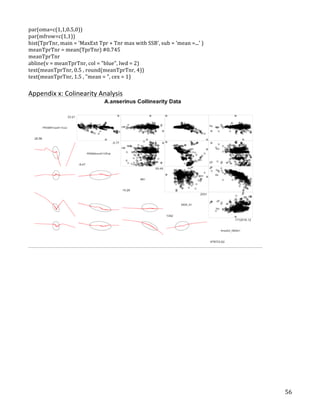
corrgram(admdata[,2:6],
order=TRUE,
lower.panel=panel.shade,
upper.panel=panel.pie,
text.panel=panel.txt,
main="A.anserinus
Collinearity
Data")
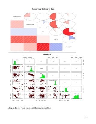
corrgram(admdata[,2:6],
order=TRUE,
lower.panel=panel.ellipse,
upper.panel=panel.pts,
text.panel=panel.txt,
diag.panel=panel.minmax,
main="A.anserinus
Collinearity
Data")
####Model
Fitting:
Generalized
Linear
Model(glm)####
gc()
#clear
garbage
from
memmory
M2
=
glm(formula=pb~.,data=admdata)
summary(M2)
##Bioclim
only
takes
presence
values
bc=
bioclim(presvals)
pairs(bc)
##Predicting
GLM
pM2
=
predict(enviropredictors,
M2,
na.rm=TRUE)
plot(pM2)
title(main
=
"Generalized
Linear
Model
Raw
Value")
summary(M2)
####
Train/Test
data
####
##get
training/testing
sets
of
data
from
admdata
head(admdata)
samp
=
sample(nrow(admdata),
round(0.75*nrow(admdata)))
traindata=admdata[samp,]
traindata=traindata[traindata[,1]
==
1,
2:7]
testdata=admdata[-­‐samp,]
pres
=
admdata[admdata[,1]
==
1,
2:7]
absen
=
admdata[admdata[,1]
==
0,
2:7]
##AUC
could
be
biased
due
to
high
extent
=
high
AUC
values
(Lobo
et
al.
2008,
Jimenez-­‐Valverde
2011)
##So,
get
rid
of
"spatial
sorting
bias"
via
"point-­‐wise
distance
sampling"
nr=nrow(Pointsxy)
s=sample(nr,0.25*nr)
pres_train=Pointsxy[-­‐s,]
pres_test=Pointsxy[s,]
nr=nrow(Absencexy)
s=sample(nr,0.25*nr)
back_train=Absencexy[-­‐s,]
back_test=Absencexy[s,]
sb=ssb(pres_test,back_test,pres_train)
sb[,1]/sb[,2]
##Spacial
Sorting
Bias
(SSB)
=
0.326
(If
no
bias
SSB=1)
##Create
subsample
where
SSB
is
removed
i
=
pwdSample(pres_test,back_test,pres_train,
n=1,tr=0.1)
pres_test_pwd=pres_test[!is.na(i[,1]),]
back_test_pwd=back_test[na.omit(as.vector(i)),]

54. 54
sb2=ssb(pres_test_pwd,back_test_pwd,pres_train)
sb2[1]/sb2[2]
##SSB
=
0.999
-­‐-­‐
Much
Reduced!
###Visualize
train/test
points
r=raster(enviropredictors,1)
plot(!is.na(r),col=c('white','light
grey'),legend=FALSE)
points(back_train,
pch='-­‐',
cex=0.5,
col=
'yellow')
points(back_test,
pch='-­‐',
cex=0.5,
col=
'black')
points(pres_train,
pch=
'+'
,
col=
'green'
)
points(pres_test,
pch=
'+'
,
col=
'blue'
)
##########
MaxEnt
##############
##Note!
Most
widely
used
SDM
algorythm
(according
to
Hijmans
and
Elith)
##limit
extent:
ext
=
extent(-­‐144.6,
-­‐113.7,
41.5,
42.3)
##Uses
"jar"
package
-­‐
http://www.cs.princeton.edu/~schapire/maxent/
jar
<-­‐
paste(system.file(package="dismo"),
"/java/maxent.jar",
sep='')
jar
if
(file.exists(jar)){
xm=maxent(enviropredictors,pres_train,
ext
=
ext)
plot(xm)
}
else
{
cat('cannot
run
this
example
because
maent
is
not
available')
plot(1)
}
response(xm)
e
=
evaluate(pres_test,back_test,xm,enviropredictors)
e
#AUC=0.7712
px=predict(enviropredictors,xm,progress='')
par(mfrow=c(1,2))
plot(px,main='MaxEnt,
Raw
Values')
trpx=threshold(e,'spec_sens')
plot(px>trpx,
main='Presence/Absence')
points(pres_train,
pch='+')
##Write
raw
data
as
raster
writeRaster(px,file="RawMaxExt.tif",overwrite=TRUE)
##Write
pres/abs
model
as
raster
MaxExtPresAbs=(px>trpx)
writeRaster(MaxExtPresAbs,file="MaxExtPresAbs.tif",overwrite=TRUE)
####
Max
Ext
Evaluation
####
e=evaluate(testdata[testdata==1,],
testdata[testdata==0,],
xm)
e
plot(e,'ROC')
##AUC
value
=
.827
(guess
@
.5)
##k-­‐fold
-­‐
do
it
agin
k
times
pres
=
admdata[admdata[,1]
==
1,
2:7]
absen
=
admdata[admdata[,1]
==
0,
2:7]
k
=
100
##I
am
going
to
run
this
10
times
group
=
kfold(pres,
k)
##presence
only,
which
is
good
becuase
the
absence
falls
very
close
##absence
is
supposed
to
be
used
to
test
model

55. 55
group[1:100]
unique(group)
e=list()
for
(i
in
1:k)
{
train=pres[group!=i,]
test=pres[group==i,]
xm=maxent(enviropredictors,pres_train)
e[[i]]=evaluate(p=test,a=absen,xm)
}
e
##AUC
values
for
sensitivity(true
positive
rate)
##
and
specificity
(true
negaitive
rate)
##With
SSB:
evaluate(xm,
p=pres_test,a=back_test,x=enviropredictors)
##AUC
with
=0.719
(0.5
is
guess)
##SSB
removed
evaluate(xm,
p=pres_test_pwd,
a=back_test_pwd,
x=enviropredictors)
##AUC
SSB
reduced
=
0.621
##These
numbers
changed
each
time
you
run
new
model,
so...
##Hist
for
AUC
with
SSB
removed
k
=
100
##I
am
going
to
run
this
100
times
group
=
kfold(pres,
k)
##presence
only,
which
is
good
becuase
the
absence
falls
very
close
##absence
is
supposed
to
be
used
to
test
model
group[1:100]
unique(group)
e=list()
for
(i
in
1:k)
{
j
=
pwdSample(pres_test,back_test,pres_train,
n=1,tr=0.1)
pres_test_pwd=pres_test[!is.na(j[,1]),]
back_test_pwd=back_test[na.omit(as.vector(j)),]
sb2=ssb(pres_test_pwd,back_test_pwd,pres_train)
xm=maxent(enviropredictors,pres_train)
e[[i]]=evaluate(xm,
p=pres_test,a=back_test,x=enviropredictors)
}
e
##AUC
values
for
sensitivity(true
positive
rate)
##
and
specificity
(true
negaitive
rate)
auc
=
sapply(e,function(x){slot(x,'auc')}
)
auc
par(mar=c(1,1,1,0))
par(oma=c(1,1,0.5,0))
par(mfrow=c(1,1))
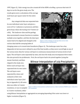
hist(auc,
main
=
'MaxExt
AUC
with
SSB',
sub
=
'mean
=
0.796')
meanauc
=
mean(auc)
#0.745
abline(v
=
meanauc,
col
=
"blue",
lwd
=
2)
text(meanauc,
0
,
round(meanauc,
4))
text(meanauc,
6
,
"mean
=
",
cex
=
1)
TprTnr
=
sapply(e,function(x){
x@t[which.max(x@TPR
+
x@TNR)]
}
)
TprTnr
par(mar=c(1,1,1,0))

56. 56
par(oma=c(1,1,0.5,0))
par(mfrow=c(1,1))
hist(TprTnr,
main
=
'MaxExt
Tpr
+
Tnr
max
with
SSB',
sub
=
'mean
=...'
)
meanTprTnr
=
mean(TprTnr)
#0.745
meanTprTnr
abline(v
=
meanTprTnr,
col
=
"blue",
lwd
=
2)
text(meanTprTnr,
0.5
,
round(meanTprTnr,
4))
text(meanTprTnr,
1.5
,
"mean
=
",
cex
=
1)
Appendix
x:
Colinearity
Analysis

57. 57
Appendix
xi:
Final
map
and
Recommendation

58. 58
nn
nn
nnnnnn
n
nnnn
nn
nn
n
WWF,USGS,EPA,Esri
Goose Creek Milkvetch Distribution Area
F
Legend
nSurveyArea
!(Astragalusanserinus
MaxEntAgrigatedModel
FinalRecomendation
MaxEnt2
MaxEnt1
CurrentRange
01.534.560.75
Miles
MaximumEntropyHabitatDistributionmodelscreatedfor
A.anserinus.AggrigatedMaxEntModelisacombination
oftwo,mostlyoverlappingMaxEntModelstobetterrepresent
empiricaldata.Finalrangecreatedbyauthoronlyas
recomendationandtoaccountforsparslypopulatedarea.
ByRobertMachol
UniversityofUtah-MST&UDAF
Dec.2014
Sources:USFWS
Allotherdatacollected2014