Machine Learning - Supervised Learning Techniques-Naïve bayes & SVM.pdf

Sanjivani Rural Education Society’s
Sanjivani College of Engineering, Kopargaon-423 603
(An Autonomous Institute, Affiliated to Savitribai Phule Pune University, Pune)
NAAC ‘A’ Grade Accredited, ISO 21001: 2018 Certified
Department of Computer Engineering
(NBA Accredited)
Subject- Machine Learning (PCCO308)
Unit 2- Supervised Learning Techniques-
Naïve bayes & SVM
Dr. B.J. Dange
Associate Professor

Contents
• Bayes‟ Theorom, Naïve Bayes‟ Classifiers,
• Naïve Bayes in Scikit- learn- Bernoulli Naïve Bayes,
• Multinomial Naïve Bayes, and Gaussian Naïve Bayes.
• Support Vector Machine(SVM)- Linear Support Vector Machines,
• Scikit- learn implementation Linear Classification,
• Kernel based classification, Non- linear Examples.
• Controlled Support Vector Machines,
• Support Vector Regression.
2
Dr.B. J. Dange, Dept. of Computer Engineering, Sanjivani CoE, Kopargaon

Naive Bayes
• It is a classification technique based on Bayes’ Theorem with an assumption of independence among
predictors.
• In simple terms, a Naive Bayes classifier assumes that the presence of a particular feature in a class
is unrelated to the presence of any other feature
• For example, a fruit may be considered to be an apple if it is red, round, and about 3 inches in diameter.
• Even if these features depend on each other or upon the existence of the other features, all of these
properties independently contribute to the probability that this fruit is an apple and that is why it is known
as ‘Naive’. ?

• Naive Bayes model is easy to build and particularly useful for very large data sets. Along with
simplicity, Naive Bayes is known to outperform even highly sophisticated classification methods.
• Bayes theorem provides a way of calculating posterior probability P(c|x) from P(c), P(x) and P(x|c).
Look at the equation below:

• Above,
• P(c|x) is the posterior probability of class (c, target) given predictor (x, attributes).
• P(c) is the prior probability of class.
• P(x|c) is the likelihood which is the probability of predictor given class.
• P(x) is the prior probability of predictor.
How Naive Bayes algorithm works?
• Let’s understand it using an example. Below I have a training data set of weather and
corresponding target variable ‘Play’ (suggesting possibilities of playing). Now, we need to classify
whether players will play or not based on weather condition.
• Let’s follow the below steps to perform it.

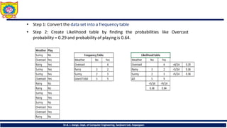
• Step 1: Convert the data set into a frequency table
• Step 2: Create Likelihood table by finding the probabilities like Overcast
probability = 0.29 and probability of playing is 0.64.

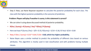
• Step 3: Now, use Naive Bayesian equation to calculate the posterior probability for each class. The
class with the highest posterior probability is the outcome of prediction.
Problem: Players will play if weather is sunny. Is this statement is correct?
• We can solve it using above discussed method of posterior probability.
• P(Yes | Sunny) = P( Sunny | Yes) * P(Yes) / P (Sunny)
• Here we have P (Sunny |Yes) = 3/9 = 0.33, P(Sunny) = 5/14 = 0.36, P( Yes)= 9/14 = 0.64
• Now, P (Yes | Sunny) = 0.33 * 0.64 / 0.36 = 0.60, which has higher probability.
• Naive Bayes uses a similar method to predict the probability of different class based on various
attributes. This algorithm is mostly used in text classification and with problems having multiple
classes.

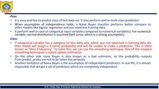
Pros:
• It is easy and fast to predict class of test data set. It also perform well in multi class prediction
• When assumption of independence holds, a Naive Bayes classifier performs better compare to
other models like logistic regression and you need less training data.
• It perform well in case of categorical input variables compared to numerical variable(s). For numerical
variable, normal distribution is assumed (bell curve, which is a strong assumption).
Cons:
• If categorical variable has a category (in test data set), which was not observed in training data set,
then model will assign a 0 (zero) probability and will be unable to make a prediction. This is often
known as “Zero Frequency”. To solve this, we can use the smoothing technique. One of the simplest
smoothing techniques is called Laplace estimation.
• On the other side naive Bayes is also known as a bad estimator, so the probability outputs
from predict_proba are not to be taken too seriously.
• Another limitation of Naive Bayes is the assumption of independent predictors. In real life, it is almost
impossible that we get a set of predictors which are completely independent.

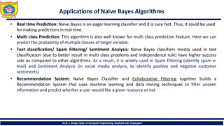
Applications of Naive Bayes Algorithms
• Real time Prediction: Naive Bayes is an eager learning classifier and it is sure fast. Thus, it could be used
for making predictions in real time.
• Multi class Prediction: This algorithm is also well known for multi class prediction feature. Here we can
predict the probability of multiple classes of target variable.
• Text classification/ Spam Filtering/ Sentiment Analysis: Naive Bayes classifiers mostly used in text
classification (due to better result in multi class problems and independence rule) have higher success
rate as compared to other algorithms. As a result, it is widely used in Spam filtering (identify spam e-
mail) and Sentiment Analysis (in social media analysis, to identify positive and negative customer
sentiments)
• Recommendation System: Naive Bayes Classifier and Collaborative Filtering together builds a
Recommendation System that uses machine learning and data mining techniques to filter unseen
information and predict whether a user would like a given resource or not

Naive Bayes Classifier
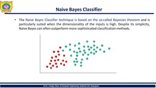
• The Naive Bayes Classifier technique is based on the so-called Bayesian theorem and is
particularly suited when the dimensionality of the inputs is high. Despite its simplicity,
Naive Bayes can often outperform more sophisticated classification methods.

• To demonstrate the concept of Naïve Bayes Classification, consider the example displayed in the
illustration above. As indicated, the objects can be classified as either GREEN or RED.
• Our task is to classify new cases as they arrive, i.e., decide to which class label they belong, based
on the currently exiting objects.
• Since there are twice as many GREEN objects as RED, it is reasonable to believe that a new case
(which hasn't been observed yet) is twice as likely to have membership GREEN rather than RED.
• In the Bayesian analysis, this belief is known as the prior probability. Prior probabilities are based
on previous experience, in this case the percentage of GREEN and RED objects, and often used to
predict outcomes before they actually happen.

Since there is a total of 60 objects, 40 of which are GREEN and 20 RED, our prior
probabilities for class membership are:

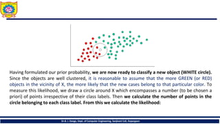
Having formulated our prior probability, we are now ready to classify a new object (WHITE circle).
Since the objects are well clustered, it is reasonable to assume that the more GREEN (or RED)
objects in the vicinity of X, the more likely that the new cases belong to that particular color. To
measure this likelihood, we draw a circle around X which encompasses a number (to be chosen a
priori) of points irrespective of their class labels. Then we calculate the number of points in the
circle belonging to each class label. From this we calculate the likelihood:

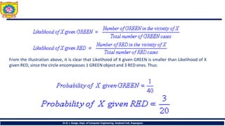
From the illustration above, it is clear that Likelihood of X given GREEN is smaller than Likelihood of X
given RED, since the circle encompasses 1 GREEN object and 3 RED ones. Thus:

• Although the prior probabilities indicate that X may belong to GREEN (given that there are twice
as many GREEN compared to RED) the likelihood indicates otherwise; that the class membership
of X is RED (given that there are more RED objects in the vicinity of X than GREEN).
• In the Bayesian analysis, the final classification is produced by combining both sources of
information, i.e., the prior and the likelihood, to form a posterior probability using the so-
called Bayes' rule (named after Rev. Thomas Bayes 1702-1761).

Finally, we classify X as RED since its class membership achieves the largest
posterior probability.
Note- The above probabilities are not normalized. However, this does not affect the
classification outcome since their normalizing constants are the same.

Technical Notes-
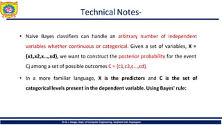
• Naive Bayes classifiers can handle an arbitrary number of independent
variables whether continuous or categorical. Given a set of variables, X =
{x1,x2,x...,xd}, we want to construct the posterior probability for the event
Cj among a set of possible outcomes C = {c1,c2,c...,cd}.
• In a more familiar language, X is the predictors and C is the set of
categorical levels present in the dependent variable. Using Bayes' rule:

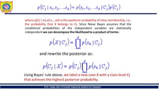
where p(Cj | x1,x2,x...,xd) is the posterior probability of class membership, i.e.,
the probability that X belongs to Cj. Since Naive Bayes assumes that the
conditional probabilities of the independent variables are statistically
independent we can decompose the likelihood to a product of terms:
and rewrite the posterior as:
Using Bayes' rule above, we label a new case X with a class level Cj
that achieves the highest posterior probability.

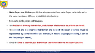
• Naive Bayes in scikit-learn- scikit-learn implements three naive Bayes variants based on
the same number of different probabilistic distributions:
• Bernoulli, multinomial, and Gaussian.
• The first one is a binary distribution, useful when a feature can be present or absent.
• The second one is a discrete distribution and is used whenever a feature must be
represented by a whole number (for example, in natural language processing, it can be
the frequency of a term),
• while the third is a continuous distribution characterized by its mean and variance.

Bernoulli naive Bayes
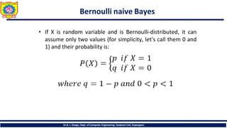
• If X is random variable and is Bernoulli-distributed, it can
assume only two values (for simplicity, let's call them 0 and
1) and their probability is:

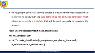
• we're going to generate a dummy dataset. Bernoulli naive Bayes expects binary
feature vectors; however, the class BernoulliNB has a binarize parameter, which
allows us to specify a threshold that will be used internally to transform the
features:
from sklearn.datasets import make_classification
>>> nb_samples = 300
>>> X, Y = make_classification(n_samples=nb_samples, n_features=2,
n_informative=2, n_redundant=0)

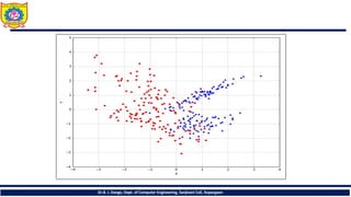
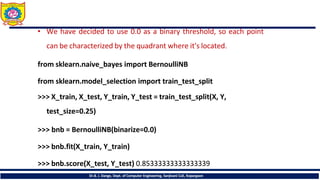
• We have decided to use 0.0 as a binary threshold, so each point
can be characterized by the quadrant where it's located.
from sklearn.naive_bayes import BernoulliNB
from sklearn.model_selection import train_test_split
>>> X_train, X_test, Y_train, Y_test = train_test_split(X, Y,
test_size=0.25)
>>> bnb = BernoulliNB(binarize=0.0)
>>> bnb.fit(X_train, Y_train)
>>> bnb.score(X_test, Y_test) 0.85333333333333339

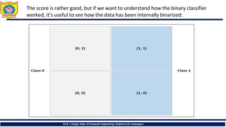
The score is rather good, but if we want to understand how the binary classifier
worked, it's useful to see how the data has been internally binarized:

• Now, checking the naive Bayes predictions, we obtain:
>>> data = np.array([[0, 0], [0, 1], [1, 0], [1, 1]])
>>> bnb.predict(data)
array([0, 0, 1, 1])
Multinomial Naive Bayes:
Feature vectors represent the frequencies with which certain events
have been generated by a multinomial distribution. This is the
event model typically used for document classification.

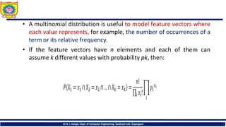
• A multinomial distribution is useful to model feature vectors where
each value represents, for example, the number of occurrences of a
term or its relative frequency.
• If the feature vectors have n elements and each of them can
assume k different values with probability pk, then:

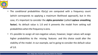
• The conditional probabilities P(xi|y) are computed with a frequency count
(which corresponds to applying a maximum likelihood approach), but in this
case, it's important to consider the alpha parameter (called Laplace smoothing
factor). Its default value is 1.0 and it prevents the model from setting null
probabilities when the frequency is zero.
• It's possible to assign all non-negative values; however, larger values will assign
higher probabilities to the missing features and this choice could alter the
stability of the model. In our example, we're going to consider the default value
of 1.0.

from sklearn.feature_extraction import DictVectorizer
>>> data = [
{'house': 100, 'street': 50, 'shop': 25, 'car': 100, 'tree': 20},
{'house': 5, 'street': 5, 'shop': 0, 'car': 10, 'tree': 500, 'river': 1} ]
>>> dv = DictVectorizer(sparse=False)
>>> X = dv.fit_transform(data)
>>> Y = np.array([1, 0])
>>> X
array([[ 100.,100., 0., 25., 50.,20.],
[10.,5.,1.,0.,5., 500.]])

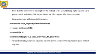
• Note that the term 'river' is missing from the first set, so it's useful to keep alpha equal to 1.0 to
give it a small probability. The output classes are 1 for city and 0 for the countryside.
• Now we can train a MultinomialNB instance:
from sklearn.naive_bayes import MultinomialNB
>>> mnb = MultinomialNB()
>>> mnb.fit(X, Y)
MultinomialNB(alpha=1.0, class_prior=None, fit_prior=True)
• To test the model, we create a dummy city with a river and a dummy countryside place without
any river:

>>> test_data = data = [
{'house': 80, 'street': 20, 'shop': 15, 'car': 70, 'tree': 10, 'river':1},
{'house': 10, 'street': 5, 'shop': 1, 'car': 8, 'tree': 300, 'river': 0}]
• >>> mnb.predict(dv.fit_transform(test_data)) array([1, 0])
• As expected, the prediction is correct.

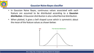
Gaussian Naive Bayes classifier
• In Gaussian Naive Bayes, continuous values associated with each
feature are assumed to be distributed according to a Gaussian
distribution. A Gaussian distribution is also called Normal distribution.
• When plotted, it gives a bell shaped curve which is symmetric about
the mean of the feature values as shown below:

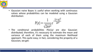
• Gaussian naive Bayes is useful when working with continuous
values whose probabilities can be modeled using a Gaussian
distribution:
• The conditional probabilities P(xi|y) are also Gaussian
distributed; therefore, it's necessary to estimate the mean and
variance of each of them using the maximum likelihood
approach. This quite easy; in fact, considering the property of a
Gaussian, we get:

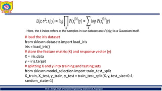
Here, the k index refers to the samples in our dataset and P(xi|y) is a Gaussian itself.
# load the iris dataset
from sklearn.datasets import load_iris
iris = load_iris()
# store the feature matrix (X) and response vector (y)
X = iris.data
y = iris.target
# splitting X and y into training and testing sets
from sklearn.model_selection import train_test_split
X_train, X_test, y_train, y_test = train_test_split(X, y, test_size=0.4,
random_state=1)

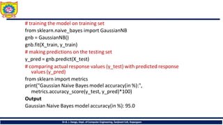
# training the model on training set
from sklearn.naive_bayes import GaussianNB
gnb = GaussianNB()
gnb.fit(X_train, y_train)
# making predictions on the testing set
y_pred = gnb.predict(X_test)
# comparing actual response values (y_test) with predicted response
values (y_pred)
from sklearn import metrics
print("Gaussian Naive Bayes model accuracy(in %):",
metrics.accuracy_score(y_test, y_pred)*100)
Output
Gaussian Naive Bayes model accuracy(in %): 95.0

Support Vector Machines
• in machine learning, support vector machines (SVMs, also support vector
networks) are supervised learning models with associated learning algorithms
that analyze data used for classification and regression analysis.
• A Support Vector Machine (SVM) is a discriminative classifier formally defined
by a separating hyperplane.
• In other words, given labeled training data (supervised learning), the
algorithm outputs an optimal hyperplane which categorizes new examples.

What is Support Vector Machine?
• An SVM model is a representation of the examples as points in space,
mapped so that the examples of the separate categories are divided by a
clear gap that is as wide as possible.
• In addition to performing linear classification, SVMs can efficiently perform a
non-linear classification, implicitly mapping their inputs into high-
dimensional feature spaces.

• “Support Vector Machine” (SVM) is a supervised machine learning algorithm
which can be used for both classification or regression challenges.
• However, it is mostly used in classification problems. In this algorithm, we
plot each data item as a point in n-dimensional space (where n is number of
features you have) with the value of each feature being the value of a particular
coordinate.
• Then, we perform classification by finding the hyper-plane that differentiate the
two classes very well (look at the below snapshot).

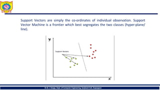
Support Vectors are simply the co-ordinates of individual observation. Support
Vector Machine is a frontier which best segregates the two classes (hyper-plane/
line).

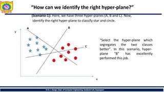
“How can we identify the right hyper-plane?”
(Scenario-1): Here, we have three hyper-planes (A, B and C). Now,
identify the right hyper-plane to classify star and circle.
“Select the hyper-plane
segregates
the two
this scenario,
which
classes
hyper-
better”. In
plane “B” has excellently
performed this job.

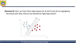
(Scenario-2): Here, we have three hyper-planes (A, B and C) and all are segregating
the classes well. Now, How can we identify the right hyper-plane?

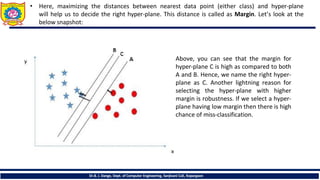
• Here, maximizing the distances between nearest data point (either class) and hyper-plane
will help us to decide the right hyper-plane. This distance is called as Margin. Let’s look at the
below snapshot:
Above, you can see that the margin for
hyper-plane C is high as compared to both
A and B. Hence, we name the right hyper-
plane as C. Another lightning reason for
selecting the hyper-plane with higher
margin is robustness. If we select a hyper-
plane having low margin then there is high
chance of miss-classification.

Some of you may have selected the hyper-plane B as it
has higher margin compared to A. But, here is
the catch, SVM selects the hyper-plane which classifies
the classes accurately prior to maximizing margin.
Here, hyper-plane B has a classification error and A has
classified all correctly. Therefore, the right hyper-plane
is A.
(Scenario-4)?: Below, I am unable to
segregate the two classes using a straight line,
as one of star lies in the territory of
other(circle) class as an outlier.

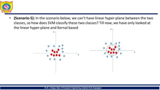
• (Scenario-5): In the scenario below, we can’t have linear hyper-plane between the two
classes, so how does SVM classify these two classes? Till now, we have only looked at
the linear hyper-plane and Kernal based

What does SVM do?
Given a set of training examples, each marked as belonging to one or
the other of two categories, an SVM training algorithm builds a
model that assigns new examples to one category or the other,
making it a non-probabilistic binary linear classifier.
Example about SVM classification of cancer UCI datasets using
machine learning tools i.e. scikit-learn compatible with Python.

# importing scikit learn with make_blobs
from sklearn.datasets.samples_generator import make_blobs
# creating datasets X containing n_samples
# Y containing two classes
X, Y = make_blobs(n_samples=500, centers=2,
random_state=0, cluster_std=0.40)
# plotting scatters
plt.scatter(X[:, 0], X[:, 1], c=Y, s=50, cmap='spring');
plt.show()

What Support vector machines do, is to not only draw a line between two
classes here, but consider a region about the line of some given width.

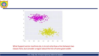
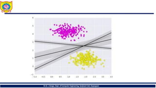
• What Support vector machines do, is to not only draw a line between two classes
here, but consider a region about the line of some given width. Here’s an
example of what it can look like:
# creating line space between -1 to 3.5
xfit = np.linspace(-1, 3.5)
# plotting scatter
plt.scatter(X[:, 0], X[:, 1], c=Y, s=50, cmap='spring')
# plot a line between the different sets of data
for m, b, d in [(1, 0.65, 0.33), (0.5, 1.6, 0.55), (-0.2, 2.9, 0.2)]:
yfit = m * xfit + b
plt.plot(xfit, yfit, '-k')
plt.fill_between(xfit, yfit - d, yfit + d, edgecolor='none',
color='#AAAAAA', alpha=0.4)
plt.xlim(-1, 3.5);
plt.show()

Importing datasets
This is the intuition of support vector machines, which optimize a linear discriminant model representing the
perpendicular distance between the datasets.
Now let’s train the classifier using our training data. Before training, we need to import cancer datasets as csv
file where we will train two features out of all features.
# importing required libraries
import numpy as np
import pandas as pd
import matplotlib.pyplot as plt
# reading csv file and extracting class column to y.
x = pd.read_csv("C:...cancer.csv")
a = np.array(x)
y = a[:,30] # classes having 0 and 1
# extracting two features
x = np.column_stack((x.malignant,x.benign))
x.shape # 569 samples and 2 features
print (x),(y)

• [[ 122.8 1001. ]
[ 132.9 1326. ]
[ 130. 1203. ] ...,
[ 108.3 858.1 ]
[ 140.1 1265. ]
[ 47.92 181. ]]
array([ 0., 0., 0., 0., 0., 0., 0., 0., 0., 0., 0., 0., 0., 0., 0., 0., 0.,
0., 0., 1., 1., 1., 0., 0., 0., 0., 0., 0., 0., 0., 0., 0., 0., 0., 0., 0.,
0., 1., 0., 0., 0., 0., 0., 0., 0., 0., 1., 0., 1., 1., 1., 1., 1., 0., 0.,
1., 0., 0., 1., 1., 1., 1., 0., 1., ...., 1.])

Fitting a Support Vector Machine
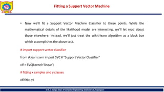
• Now we’ll fit a Support Vector Machine Classifier to these points. While the
mathematical details of the likelihood model are interesting, we’ll let read about
those elsewhere. Instead, we’ll just treat the scikit-learn algorithm as a black box
which accomplishes the above task.
# import support vector classifier
from sklearn.svm import SVC # "Support Vector Classifier"
clf = SVC(kernel='linear')
# fitting x samples and y classes
clf.fit(x, y)

• After being fitted, the model can then be used to predict new values:
clf.predict([[120, 990]])
clf.predict([[85, 550]])
array([ 0.]) array([ 1.])
This is obtained by analyzing
the data taken and pre-
processing methods to
make optimal hyperplanes
using matplotlib function.

Kernel Methods and Nonlinear Classification
Often we want to capture nonlinear patterns in the data
Nonlinear Regression: Input-output relationship may not be linear
Nonlinear Classification: Classes may not be separable by a linear
boundary

Input-output relationship may not be
Classes may not be separable by a
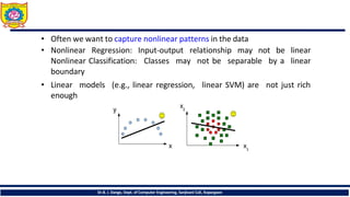
• Often we want to capture nonlinear patterns in the data
• Nonlinear Regression:
Nonlinear Classification:
boundary
linear
linear
• Linear models (e.g., linear regression, linear SVM) are not just rich
enough

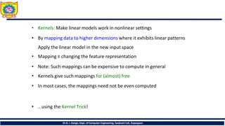
• Kernels: Make linear models work in nonlinear settings
• By mapping data to higher dimensions where it exhibits linear patterns
Apply the linear model in the new input space
• Mapping ≡ changing the feature representation
• Note: Such mappings can be expensive to compute in general
• Kernels give such mappings for (almost) free
• In most cases, the mappings need not be even computed
• .. using the Kernel Trick!

Classifying non-linearly separable data
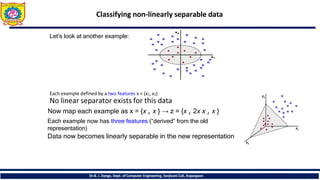
Let’s look at another example:
Each example defined by a two features x = {x1, x2}
No linear separator exists for this data
Now map each example as x = {x , x } → z = {x , 2x x , x }
Each example now has three features (“derived” from the old
representation)
Data now becomes linearly separable in the new representation

Feature Mapping
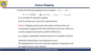
Consider the following mapping φ for an example x = {x1, . . . , xD }
1 2 D 1 2 1 2 1 D D−1 D
φ : x → {x 2
, x 2
, . . . , x2, , x x , x x , . . . , x x , . . . . . . , x x }
It’s an example of a quadratic mapping
Each new feature uses a pair of the original features
Problem: Mapping usually leads to the number of features blow up!
Computing the mapping itself can be inefficient in such cases Moreover,
using the mapped representation could be inefficient too
e.g., imagine computing the similarity between two examples: φ(x)𝖳φ(z)
Thankfully, Kernels help us avoid both these issues!
The mapping doesn’t have to be explicitly computed Computations with
the mapped features remain efficient

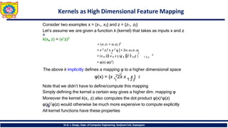
Kernels as High Dimensional Feature Mapping
Consider two examples x = {x1, x2} and z = {z1, z2}
Let’s assume we are given a function k (kernel) that takes as inputs x and z
k(x, z) = (x𝖳z)2
= (x1 z1 + x2 z2 )2
= x 2 z 2 + x 2 z 2 + 2x1 x2 z1 z2
2 2 𝖳 2
1 1 2 2 1
1 1
√
2 2
√ 2
1 2 2
= (x , 2x x , x ) (z , 2z z , z )
= φ(x) φ(z𝖳
)
The above k implicitly defines a mapping φ to a higher dimensional space
√ 2
φ(x) = {x ,22x x , x }
1 1 2 2
Note that we didn’t have to define/compute this mapping
Simply defining the kernel a certain way gives a higher dim. mapping φ
Moreover the kernel k(x, z) also computes the dot product φ(x)𝖳φ(z)
φ(x)𝖳φ(z) would otherwise be much more expensive to compute explicitly
All kernel functions have these properties

Kernels: Formally Defined
Recall: Each kernel k has an associated feature mapping φ
φ takes input x ∈ X (input space) and maps it to F (“feature space”)
Kernel k(x, z) takes two inputs and gives their similarity in F space
φ : X → F
k : X × X → R, k(x, z) = φ(x)𝖳φ(z)
F needs to be a vector space with a dot product defined on it
Also called a Hilbert Space
Can just any function be used as a kernel function?
No. It must satisfy Mercer’s Condition

For k to be a kernel function
There must exist a Hilbert Space F for which k defines a dot product
The above is true if K is a positive definite function
∫ ∫
d x d zf (x)k(x, z)f (z) > 0 (∀f ∈ L2)
This is Mercer’s Condition
Let k1, k2 be two kernel functions then the following are as well:
k(x, z) = k1(x, z) + k2(x, z): direct sum
k(x, z) = αk1(x, z): scalar product
k(x, z) = k1(x, z)k2(x, z): direct product
Kernels can also be constructed by composing these
rules
Mercer’s Condition
Mercer’s Condition

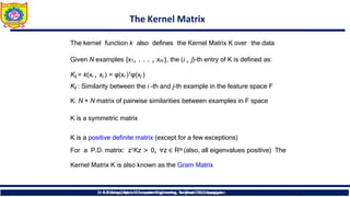
The Kernel Matrix
The kernel function k also defines the Kernel Matrix K over the data
Given N examples {x1, . . . , xN }, the (i , j)-th entry of K is defined as:
Kij = k(xi , xj ) = φ(xi )𝖳φ(xj )
Kij : Similarity between the i -th and j-th example in the feature space F
K: N × N matrix of pairwise similarities between examples in F space
K is a symmetric matrix
K is a positive definite matrix (except for a few exceptions)
For a P.D. matrix: z𝖳Kz > 0, ∀z ∈ RN (also, all eigenvalues positive) The
Kernel Matrix K is also known as the Gram Matrix
9 16
Dr.T.Bhaskar,Dept. of Computer Engineering, Sanjivani CoE, Kopargaon

Some Examples of Kernels
The following are the most popular kernels for real-valued vector
inputs Linear (trivial) Kernel:
k(x, z) = x𝖳z (mapping function φ is identity - no mapping) Quadratic
Kernel:
or (1 + x𝖳z)2
or (1 + x𝖳z)d
k(x, z) = (x𝖳z)2
Polynomial Kernel (of degree d ):
k(x, z) = (x𝖳z)d
Radial Basis Function (RBF)
Kernel:
k(x, z) = exp[−γ||x − z||2]
γ is a hyperparameter (also called the kernel bandwidth)
The RBF kernel corresponds to an infinite dimensional
feature space F (i.e., you can’t actually write down the
vector φ(x))
Note: Kernel hyperparameters (e.g., d , γ) chosen via
cross-validation

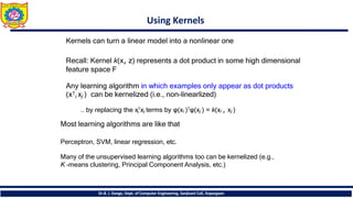
Using Kernels
Kernels can turn a linear model into a nonlinear one
Recall: Kernel k(x, z) represents a dot product in some high dimensional
feature space F
Any learning algorithm in which examples only appear as dot products
(x𝖳
i xj ) can be kernelized (i.e., non-linearlized)
i
.. by replacing the x𝖳xj terms by φ(xi )𝖳φ(xj ) = k(xi , xj )
Most learning algorithms are like that
Perceptron, SVM, linear regression, etc.
Many of the unsupervised learning algorithms too can be kernelized (e.g.,
K -means clustering, Principal Component Analysis, etc.)

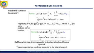
Kernelized SVM Training
Recall the SVM dual
Lagrangian: ΣN 1 Σ
N
Maximize LD(w, b, ξ, α, β) = αn −
n=1 2 m,n=1
m n
αm
α y
n ym(xnx )T
N
Σ
subject to αn yn = 0, 0 ≤ αn ≤ C ; n = 1, . . .
, N
n=1
m
T 𝖳
Replacing x x by φ(x ) φ(x ) = k(x , x ) = K
n m n m n mn , where k(., .) is
some
suitable kernel
function N
n=1
Σ N
Maximize LD (w, b, ξ, α, β) = αn − 2
Σ 1
αm αn ym yn Kmn
m,n=1
N
Σ
subject to αn yn = 0, 0 ≤ αn ≤ C ; n = 1, . . .
, N
n=1
SVM now learns a linear separator in the kernel defined feature
space F
This corresponds to a non-linear separator in the original space X
Dr.B. J. Dange, Dept.of Computer Engineering,SanjivaniCoE, Kopargaon

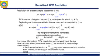
Kernelized SVM Prediction
Prediction for a test example x (assume b = 0)
Σ
y = sign(w 𝖳
x) = sign( αny
n nx 𝖳
x)
n∈SV
SV is the set of support vectors (i.e., examples for which αn > 0)
Replacing each example with its feature mapped representation (x →
φ(x)) Σ Σ
y = sign( αnynφ(xn ) φ(x)) = sign( αnynk(x ,
n x))
𝖳
n∈SV n∈SV
The weight vector for the kernelized
case can be expressed as:
w
Σ = αnynφ(xn) = αny
Σ
n
k(x ,
n .)
n∈SV n∈SV
Important: Kernelized SVM needs the support vectors at the test
time (except when you can write φ(xn ) as an explicit, reasonably-
sized vector)
In the unkernelized version w
Σ
n∈SV αny
n n
x can be computed and stored as
a
= D × 1 vector, so the support vectors need not be
stored

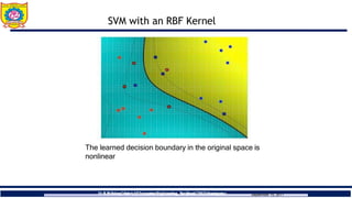
SVM with an RBF Kernel
The learned decision boundary in the original space is
nonlinear
September 15, 2011
Dr.T.Bhaskar,Dept. of Computer Engineering, Sanjivani CoE, Kopargaon

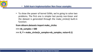
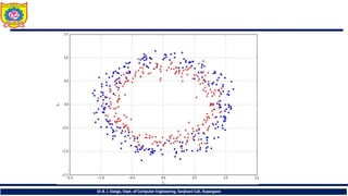
• Scikit-learn-implementation Non-linear examples
• To show the power of kernel SVMs, we're going to solve two
problems. The first one is simpler but purely non-linear and
the dataset is generated through the make_circles() built-in
function:
from sklearn.datasets import make_circles
>>> nb_samples = 500
>>> X, Y = make_circles(n_samples=nb_samples, noise=0.1)

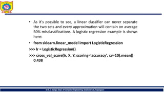
• As it's possible to see, a linear classifier can never separate
the two sets and every approximation will contain on average
50% misclassifications. A logistic regression example is shown
here:
• from sklearn.linear_model import LogisticRegression
>>> lr = LogisticRegression()
>>> cross_val_score(lr, X, Y, scoring='accuracy', cv=10).mean()
0.438

• As expected, the accuracy is below 50% and no other optimizations can
increase it dramatically. Let's consider, instead, a grid search with an
SVM and different kernels (keeping the default values of each one):
import multiprocessing
from sklearn.model_selection import GridSearchCV
>>> param_grid = [
{ 'kernel': ['linear', 'rbf', 'poly', 'sigmoid'],
'C': [ 0.1, 0.2, 0.4, 0.5, 1.0, 1.5, 1.8, 2.0, 2.5, 3.0 ]
} ]
>>> gs = GridSearchCV(estimator=SVC(), param_grid=param_grid,
scoring='accuracy', cv=10,

n_jobs=multiprocessing.cpu_count())
>>> gs.fit(X, Y)
GridSearchCV(cv=10, error_score='raise‘,estimator=SVC(C=1.0, cache_size=200,
class_weight=None, coef0=0.0, decision_function_shape=None, degree=3, gamma='auto',
kernel='rbf', max_iter=-1, probability=False, random_state=None, shrinking=True, tol=0.001,
verbose=False), fit_params={}, iid=True, n_jobs=8,param_grid=[{'kernel': ['linear', 'rbf', 'poly',
'sigmoid'], 'C‘:[0.1, 0.2, 0.4, 0.5, 1.0, 1.5, 1.8, 2.0, 2.5, 3.0]}],pre_dispatch='2*n_jobs',
refit=True, return_train_score=True, scoring='accuracy', verbose=0)
>>> gs.best_estimator_
SVC(C=2.0, cache_size=200, class_weight=None, coef0=0.0, decision_function_shape=None,
degree=3, gamma='auto', kernel='rbf', max_iter=-1, probability=False, random_state=None,
shrinking=True, tol=0.001, verbose=False)
>>> gs.best_score_
0.87
As expected from the geometry of our dataset, the best kernel is a radial basis function, which
yields 87% accuracy.
So the best estimator is polynomial-based with degree=2, and the corresponding accuracy is:
0.96

Controlled support vector machines
• With real datasets, SVM can extract a very large number of support vectors to
increase accuracy, and that can slow down the whole process.
• To allow finding out a trade-off between precision and number of support
vectors, scikit-learn provides an implementation called NuSVC, where the
parameter nu (bounded between 0—not included—and 1) can be used to control
at the same time the number of support vectors (greater values will increase their
number) and training errors (lower values reduce the fraction of errors).
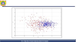
• Let's consider an example with a linear kernel and a simple dataset. In the
following figure, there's a scatter plot of our set:

• Let's start checking the number of support vectors for a standard SVM:
>>> svc = SVC(kernel='linear')
>>> svc.fit(X, Y)
>>> svc.support_vectors_.shape (242L, 2L)
>>> cross_val_score(nusvc, X, Y,scoring='accuracy', cv=10).mean()
0.80633213285314143
• As expected, the behavior is similar to a standard SVC. Let's now reduce
the value of nu:
>>> nusvc = NuSVC(kernel='linear', nu=0.15)
>>> nusvc.fit(X, Y)
>>> nusvc.support_vectors_.shape (78L, 2L)
>>> cross_val_score(nusvc, X, Y,scoring='accuracy', cv=10).mean()
0.67584393757503003

• In this case, the number of support vectors is less than before and also the
accuracy has been affected by this choice. Instead of trying different values,
we can look for the best choice with a grid search:
import numpy as np
>>> param_grid = [
{ 'nu': np.arange(0.05, 1.0, 0.05) } ]
>>> gs = GridSearchCV(estimator=NuSVC(kernel='linear'),
param_grid=param_grid, scoring='accuracy', cv=10,
n_jobs=multiprocessing.cpu_count())

>>> gs.fit(X, Y)
GridSearchCV(cv=10, error_score='raise', estimator=NuSVC(cache_size=200,
class_weight=None, coef0=0.0, decision_function_shape=None, degree=3,
gamma='auto', kernel='linear', max_iter=-1, nu=0.5, probability=False,
random_state=None, shrinking=True, tol=0.001, verbose=False), fit_params={},
iid=True, n_jobs=8, param_grid=[{'nu': array([ 0.05, 0.1 , 0.15, 0.2 , 0.25,
0.8 , 0.85,
0.3
0.9 ,
,0.35, 0.4 , 0.45, 0.5 , 0.55, 0.6 , 0.65, 0.7 , 0.75,
0.95])}],
pre_dispatch='2*n_jobs', refit=True, return_train_score=True, scoring='accuracy',
verbose=0)
>>> gs.best_estimator_
• NuSVC(cache_size=200, class_weight=None, coef0=0.0,
decision_function_shape=None, degree=3, gamma='auto', kernel='linear', max_iter=-1,
nu=0.5, probability=False, random_state=None, shrinking=True, tol=0.001,
verbose=False)
>>> gs.best_score_ 0.80600000000000005
>>> gs.best_estimator_.support_vectors_.shape (251L, 2L) Therefore, in this case as
well, the default value of 0.5 yielded the most accurate results.

Support vector regression
• algorithm already described (see the original documentation for
further information). The real power of this approach resides in the
usage of non-linear kernels (in particular, polynomials); however, the
user is advised to evaluate the degree progressively because the
complexity can grow rapidly, together with the training time.
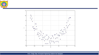
• For our example, I've created a dummy dataset based on a second-
order noisy function:

>>> nb_samples = 50
>>> X = np.arange(-nb_samples, nb_samples, 1)
>>> Y = np.zeros(shape=(2 * nb_samples,))
>>> for x in X:
Y[int(x)+nb_samples] = np.power(x*6, 2.0) / 1e4 +
np.random.uniform(-2, 2)

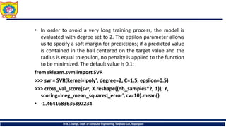
• In order to avoid a very long training process, the model is
evaluated with degree set to 2. The epsilon parameter allows
us to specify a soft margin for predictions; if a predicted value
is contained in the ball centered on the target value and the
radius is equal to epsilon, no penalty is applied to the function
to be minimized. The default value is 0.1:
from sklearn.svm import SVR
>>> svr = SVR(kernel='poly', degree=2, C=1.5, epsilon=0.5)
>>> cross_val_score(svr, X.reshape((nb_samples*2, 1)), Y,
scoring='neg_mean_squared_error', cv=10).mean()
• -1.4641683636397234

Thank You

Machine Learning - Supervised Learning Techniques-Naïve bayes & SVM.pdf

More Related Content

Similar to Machine Learning - Supervised Learning Techniques-Naïve bayes & SVM.pdf

More from BapusahebDange

Recently uploaded

Machine Learning - Supervised Learning Techniques-Naïve bayes & SVM.pdf