M and B 3 3rd Edition Dean Croushore Solutions Manual
M and B 3 3rd Edition Dean Croushore Solutions Manual
M and B 3 3rd Edition Dean Croushore Solutions Manual
M and B 3 3rd Edition Dean Croushore Solutions Manual
M and B 3 3rd Edition Dean Croushore Solutions Manual
1.
M and B3 3rd Edition Dean Croushore Solutions
Manual download
https://testbankdeal.com/product/m-and-b-3-3rd-edition-dean-
croushore-solutions-manual/
Visit testbankdeal.com today to download the complete set of
test bank or solution manual
2.
We believe theseproducts will be a great fit for you. Click
the link to download now, or visit testbankdeal.com
to discover even more!
M and B 3 Hybrid 3rd Edition Dean Croushore Solutions
Manual
https://testbankdeal.com/product/m-and-b-3-hybrid-3rd-edition-dean-
croushore-solutions-manual/
M and B 3 3rd Edition Dean Croushore Test Bank
https://testbankdeal.com/product/m-and-b-3-3rd-edition-dean-croushore-
test-bank/
ORGB 3 3rd Edition Nelson Solutions Manual
https://testbankdeal.com/product/orgb-3-3rd-edition-nelson-solutions-
manual/
Fundamentals of Law Office Management 5th Edition
Nollkamper Test Bank
https://testbankdeal.com/product/fundamentals-of-law-office-
management-5th-edition-nollkamper-test-bank/
3.
Auditing And AssuranceServices In Australia 6th Edition
Louwers Solutions Manual
https://testbankdeal.com/product/auditing-and-assurance-services-in-
australia-6th-edition-louwers-solutions-manual/
Statistics For Managers Using Microsoft Excel 7th Edition
Levine Solutions Manual
https://testbankdeal.com/product/statistics-for-managers-using-
microsoft-excel-7th-edition-levine-solutions-manual/
Management of Strategy Concepts International Edition 10th
Edition Ireland Solutions Manual
https://testbankdeal.com/product/management-of-strategy-concepts-
international-edition-10th-edition-ireland-solutions-manual/
We The People 12th Edition Ginsberg Test Bank
https://testbankdeal.com/product/we-the-people-12th-edition-ginsberg-
test-bank/
Principles of Finance 6th Edition Besley Solutions Manual
https://testbankdeal.com/product/principles-of-finance-6th-edition-
besley-solutions-manual/
4.
Educational Psychology Theoryand Practice 10th Edition
Slavin Test Bank
https://testbankdeal.com/product/educational-psychology-theory-and-
practice-10th-edition-slavin-test-bank/
This eBook isfor the use of anyone anywhere in the United
States and most other parts of the world at no cost and with
almost no restrictions whatsoever. You may copy it, give it away
or re-use it under the terms of the Project Gutenberg License
included with this eBook or online at www.gutenberg.org. If you
are not located in the United States, you will have to check the
laws of the country where you are located before using this
eBook.
1.E.2. If an individual Project Gutenberg™ electronic work is derived
from texts not protected by U.S. copyright law (does not contain a
notice indicating that it is posted with permission of the copyright
holder), the work can be copied and distributed to anyone in the
United States without paying any fees or charges. If you are
redistributing or providing access to a work with the phrase “Project
Gutenberg” associated with or appearing on the work, you must
comply either with the requirements of paragraphs 1.E.1 through
1.E.7 or obtain permission for the use of the work and the Project
Gutenberg™ trademark as set forth in paragraphs 1.E.8 or 1.E.9.
1.E.3. If an individual Project Gutenberg™ electronic work is posted
with the permission of the copyright holder, your use and distribution
must comply with both paragraphs 1.E.1 through 1.E.7 and any
additional terms imposed by the copyright holder. Additional terms
will be linked to the Project Gutenberg™ License for all works posted
with the permission of the copyright holder found at the beginning
of this work.
1.E.4. Do not unlink or detach or remove the full Project
Gutenberg™ License terms from this work, or any files containing a
part of this work or any other work associated with Project
Gutenberg™.
1.E.5. Do not copy, display, perform, distribute or redistribute this
electronic work, or any part of this electronic work, without
prominently displaying the sentence set forth in paragraph 1.E.1
19.
with active linksor immediate access to the full terms of the Project
Gutenberg™ License.
1.E.6. You may convert to and distribute this work in any binary,
compressed, marked up, nonproprietary or proprietary form,
including any word processing or hypertext form. However, if you
provide access to or distribute copies of a Project Gutenberg™ work
in a format other than “Plain Vanilla ASCII” or other format used in
the official version posted on the official Project Gutenberg™ website
(www.gutenberg.org), you must, at no additional cost, fee or
expense to the user, provide a copy, a means of exporting a copy, or
a means of obtaining a copy upon request, of the work in its original
“Plain Vanilla ASCII” or other form. Any alternate format must
include the full Project Gutenberg™ License as specified in
paragraph 1.E.1.
1.E.7. Do not charge a fee for access to, viewing, displaying,
performing, copying or distributing any Project Gutenberg™ works
unless you comply with paragraph 1.E.8 or 1.E.9.
1.E.8. You may charge a reasonable fee for copies of or providing
access to or distributing Project Gutenberg™ electronic works
provided that:
• You pay a royalty fee of 20% of the gross profits you derive
from the use of Project Gutenberg™ works calculated using the
method you already use to calculate your applicable taxes. The
fee is owed to the owner of the Project Gutenberg™ trademark,
but he has agreed to donate royalties under this paragraph to
the Project Gutenberg Literary Archive Foundation. Royalty
payments must be paid within 60 days following each date on
which you prepare (or are legally required to prepare) your
periodic tax returns. Royalty payments should be clearly marked
as such and sent to the Project Gutenberg Literary Archive
Foundation at the address specified in Section 4, “Information
20.
about donations tothe Project Gutenberg Literary Archive
Foundation.”
• You provide a full refund of any money paid by a user who
notifies you in writing (or by e-mail) within 30 days of receipt
that s/he does not agree to the terms of the full Project
Gutenberg™ License. You must require such a user to return or
destroy all copies of the works possessed in a physical medium
and discontinue all use of and all access to other copies of
Project Gutenberg™ works.
• You provide, in accordance with paragraph 1.F.3, a full refund of
any money paid for a work or a replacement copy, if a defect in
the electronic work is discovered and reported to you within 90
days of receipt of the work.
• You comply with all other terms of this agreement for free
distribution of Project Gutenberg™ works.
1.E.9. If you wish to charge a fee or distribute a Project Gutenberg™
electronic work or group of works on different terms than are set
forth in this agreement, you must obtain permission in writing from
the Project Gutenberg Literary Archive Foundation, the manager of
the Project Gutenberg™ trademark. Contact the Foundation as set
forth in Section 3 below.
1.F.
1.F.1. Project Gutenberg volunteers and employees expend
considerable effort to identify, do copyright research on, transcribe
and proofread works not protected by U.S. copyright law in creating
the Project Gutenberg™ collection. Despite these efforts, Project
Gutenberg™ electronic works, and the medium on which they may
be stored, may contain “Defects,” such as, but not limited to,
incomplete, inaccurate or corrupt data, transcription errors, a
copyright or other intellectual property infringement, a defective or
21.
damaged disk orother medium, a computer virus, or computer
codes that damage or cannot be read by your equipment.
1.F.2. LIMITED WARRANTY, DISCLAIMER OF DAMAGES - Except for
the “Right of Replacement or Refund” described in paragraph 1.F.3,
the Project Gutenberg Literary Archive Foundation, the owner of the
Project Gutenberg™ trademark, and any other party distributing a
Project Gutenberg™ electronic work under this agreement, disclaim
all liability to you for damages, costs and expenses, including legal
fees. YOU AGREE THAT YOU HAVE NO REMEDIES FOR
NEGLIGENCE, STRICT LIABILITY, BREACH OF WARRANTY OR
BREACH OF CONTRACT EXCEPT THOSE PROVIDED IN PARAGRAPH
1.F.3. YOU AGREE THAT THE FOUNDATION, THE TRADEMARK
OWNER, AND ANY DISTRIBUTOR UNDER THIS AGREEMENT WILL
NOT BE LIABLE TO YOU FOR ACTUAL, DIRECT, INDIRECT,
CONSEQUENTIAL, PUNITIVE OR INCIDENTAL DAMAGES EVEN IF
YOU GIVE NOTICE OF THE POSSIBILITY OF SUCH DAMAGE.
1.F.3. LIMITED RIGHT OF REPLACEMENT OR REFUND - If you
discover a defect in this electronic work within 90 days of receiving
it, you can receive a refund of the money (if any) you paid for it by
sending a written explanation to the person you received the work
from. If you received the work on a physical medium, you must
return the medium with your written explanation. The person or
entity that provided you with the defective work may elect to provide
a replacement copy in lieu of a refund. If you received the work
electronically, the person or entity providing it to you may choose to
give you a second opportunity to receive the work electronically in
lieu of a refund. If the second copy is also defective, you may
demand a refund in writing without further opportunities to fix the
problem.
1.F.4. Except for the limited right of replacement or refund set forth
in paragraph 1.F.3, this work is provided to you ‘AS-IS’, WITH NO
OTHER WARRANTIES OF ANY KIND, EXPRESS OR IMPLIED,
22.
INCLUDING BUT NOTLIMITED TO WARRANTIES OF
MERCHANTABILITY OR FITNESS FOR ANY PURPOSE.
1.F.5. Some states do not allow disclaimers of certain implied
warranties or the exclusion or limitation of certain types of damages.
If any disclaimer or limitation set forth in this agreement violates the
law of the state applicable to this agreement, the agreement shall be
interpreted to make the maximum disclaimer or limitation permitted
by the applicable state law. The invalidity or unenforceability of any
provision of this agreement shall not void the remaining provisions.
1.F.6. INDEMNITY - You agree to indemnify and hold the Foundation,
the trademark owner, any agent or employee of the Foundation,
anyone providing copies of Project Gutenberg™ electronic works in
accordance with this agreement, and any volunteers associated with
the production, promotion and distribution of Project Gutenberg™
electronic works, harmless from all liability, costs and expenses,
including legal fees, that arise directly or indirectly from any of the
following which you do or cause to occur: (a) distribution of this or
any Project Gutenberg™ work, (b) alteration, modification, or
additions or deletions to any Project Gutenberg™ work, and (c) any
Defect you cause.
Section 2. Information about the Mission
of Project Gutenberg™
Project Gutenberg™ is synonymous with the free distribution of
electronic works in formats readable by the widest variety of
computers including obsolete, old, middle-aged and new computers.
It exists because of the efforts of hundreds of volunteers and
donations from people in all walks of life.
Volunteers and financial support to provide volunteers with the
assistance they need are critical to reaching Project Gutenberg™’s
goals and ensuring that the Project Gutenberg™ collection will
23.
remain freely availablefor generations to come. In 2001, the Project
Gutenberg Literary Archive Foundation was created to provide a
secure and permanent future for Project Gutenberg™ and future
generations. To learn more about the Project Gutenberg Literary
Archive Foundation and how your efforts and donations can help,
see Sections 3 and 4 and the Foundation information page at
www.gutenberg.org.
Section 3. Information about the Project
Gutenberg Literary Archive Foundation
The Project Gutenberg Literary Archive Foundation is a non-profit
501(c)(3) educational corporation organized under the laws of the
state of Mississippi and granted tax exempt status by the Internal
Revenue Service. The Foundation’s EIN or federal tax identification
number is 64-6221541. Contributions to the Project Gutenberg
Literary Archive Foundation are tax deductible to the full extent
permitted by U.S. federal laws and your state’s laws.
The Foundation’s business office is located at 809 North 1500 West,
Salt Lake City, UT 84116, (801) 596-1887. Email contact links and up
to date contact information can be found at the Foundation’s website
and official page at www.gutenberg.org/contact
Section 4. Information about Donations to
the Project Gutenberg Literary Archive
Foundation
Project Gutenberg™ depends upon and cannot survive without
widespread public support and donations to carry out its mission of
increasing the number of public domain and licensed works that can
be freely distributed in machine-readable form accessible by the
widest array of equipment including outdated equipment. Many
24.
small donations ($1to $5,000) are particularly important to
maintaining tax exempt status with the IRS.
The Foundation is committed to complying with the laws regulating
charities and charitable donations in all 50 states of the United
States. Compliance requirements are not uniform and it takes a
considerable effort, much paperwork and many fees to meet and
keep up with these requirements. We do not solicit donations in
locations where we have not received written confirmation of
compliance. To SEND DONATIONS or determine the status of
compliance for any particular state visit www.gutenberg.org/donate.
While we cannot and do not solicit contributions from states where
we have not met the solicitation requirements, we know of no
prohibition against accepting unsolicited donations from donors in
such states who approach us with offers to donate.
International donations are gratefully accepted, but we cannot make
any statements concerning tax treatment of donations received from
outside the United States. U.S. laws alone swamp our small staff.
Please check the Project Gutenberg web pages for current donation
methods and addresses. Donations are accepted in a number of
other ways including checks, online payments and credit card
donations. To donate, please visit: www.gutenberg.org/donate.
Section 5. General Information About
Project Gutenberg™ electronic works
Professor Michael S. Hart was the originator of the Project
Gutenberg™ concept of a library of electronic works that could be
freely shared with anyone. For forty years, he produced and
distributed Project Gutenberg™ eBooks with only a loose network of
volunteer support.
25.
Project Gutenberg™ eBooksare often created from several printed
editions, all of which are confirmed as not protected by copyright in
the U.S. unless a copyright notice is included. Thus, we do not
necessarily keep eBooks in compliance with any particular paper
edition.
Most people start at our website which has the main PG search
facility: www.gutenberg.org.
This website includes information about Project Gutenberg™,
including how to make donations to the Project Gutenberg Literary
Archive Foundation, how to help produce our new eBooks, and how
to subscribe to our email newsletter to hear about new eBooks.
26.
Welcome to ourwebsite – the perfect destination for book lovers and
knowledge seekers. We believe that every book holds a new world,
offering opportunities for learning, discovery, and personal growth.
That’s why we are dedicated to bringing you a diverse collection of
books, ranging from classic literature and specialized publications to
self-development guides and children's books.
More than just a book-buying platform, we strive to be a bridge
connecting you with timeless cultural and intellectual values. With an
elegant, user-friendly interface and a smart search system, you can
quickly find the books that best suit your interests. Additionally,
our special promotions and home delivery services help you save time
and fully enjoy the joy of reading.
Join us on a journey of knowledge exploration, passion nurturing, and
personal growth every day!
testbankdeal.com


![Chapter 10: Economic Growth and Business Cycles 106
© 2015 Cengage Learning. All Rights Reserved. May not be copied, scanned, or duplicated, in whole or in part, except for use as permitted in
a license distributed with a certain product or service or otherwise on a password-protected website for classroom use
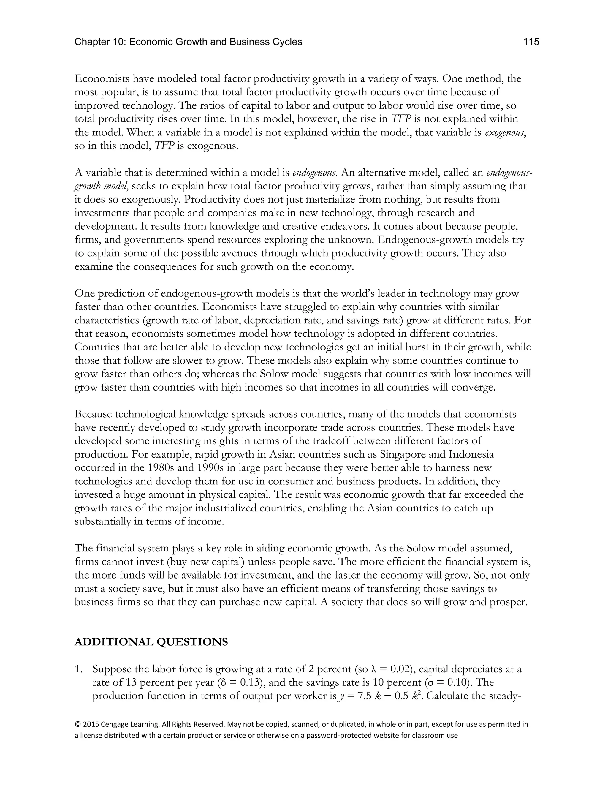
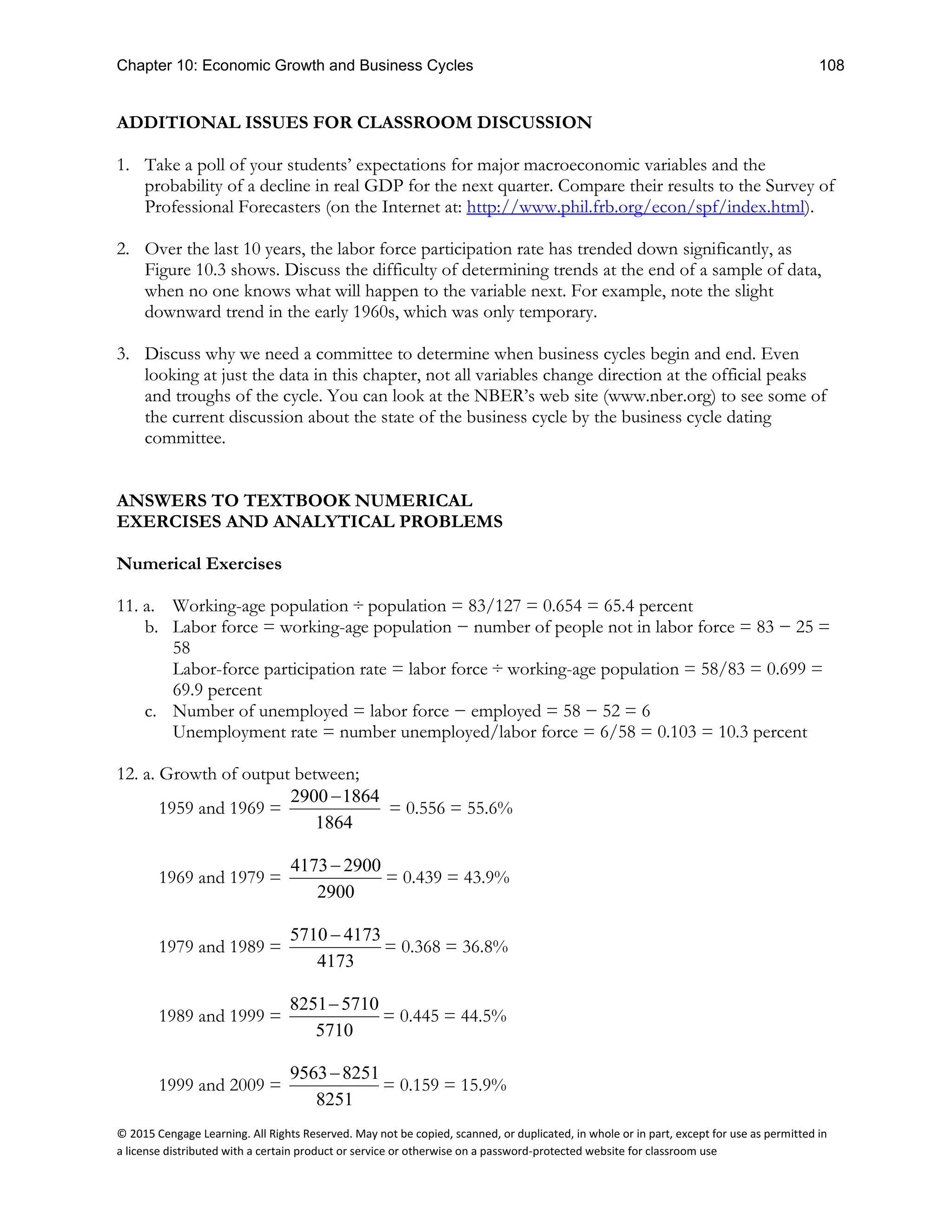
d) Population is split into working-age population and others (too young, in military, in
institutions); working-age population = labor force + not in labor force; labor force =
employed + unemployed (Figure 10.4); unemployment rate = unemployed ÷ labor
force (Figure 10.5)
e) Labor productivity = output ÷ number of hours worked (Figures 10.6 and 10.7)
f) Output growth = labor productivity growth + growth in hours worked
g) Economic Liftoff is the period from 1950 to 1970; Reorganization is the period from
1971 to 1982; Long Boom is the period from 1983 to 2007 (Table 10.1; Figure 10.8);
what will be the effect of the financial crisis of 2008? Use Data Bank: Why Is the
Economy More Stable in the Long Boom?
3. A View of Economic Growth Using Data on Both Labor and Capital
a) Economy’s production function: production mainly depends on capital and labor:
Y =F(K,L) (3)
b) A specific production function fits the data well:
Y =A × Ka
× L1−a
(4)
(1) The term A is a measure of the economy’s total factor productivity, TFP
(2) The growth-rate form of equation (4) shows how TFP growth contributes to
output growth:
%ΔY = %ΔA + (a × %ΔK) + [(1 − a) × %ΔL]
Output growth = TFP growth + [a × growth rate of capital] (5)
+ [(1 – a) × growth rate of labor]
(3) TFP growth is calculated using equation (5):
%ΔA = %ΔY − [a × %ΔK] − [(1 – a) × %ΔL] (6)
(3) It is vital to remember that the data on capital are questionable, so calculations of
TFP may be far from accurate
c) Table 10.2 shows the breakdown of growth in the three periods (Economic Liftoff,
Reorganization, and Long Boom); TFP growth changes over those periods in a similar
way to growth in labor productivity
C. Data Bank: Why Is the Economy More Stable in the Long Boom?
1. Research by Stock and Watson suggests that the economy became more stable at the start
of the Long Boom (Figure 10.A)
2. Better monetary policy is responsible for just a fraction of the increased stability; the rest
may be just good luck
D. Business Cycles
1. What Is a Business Cycle?
a) A business cycle is the short-term movement of output and other key economic
variables (such as income and employment) around their long-term trends; use Figure
10.9 to illustrate a hypothetical business cycle
b) Define economic expansion and peak, recession and depression, and trough
c) The NBER’s business cycle dating committee determines when recessions and
expansions begin and end (Figure 10.9 and Table 10.3)
d) A business cycle has two main characteristics (Figure 10.10):](https://image.slidesharecdn.com/17458-250704033124-a2c9edc9/75/M-and-B-3-3rd-Edition-Dean-Croushore-Solutions-Manual-6-2048.jpg)
![Chapter 10: Economic Growth and Business Cycles 109
© 2015 Cengage Learning. All Rights Reserved. May not be copied, scanned, or duplicated, in whole or in part, except for use as permitted in
a license distributed with a certain product or service or otherwise on a password-protected website for classroom use
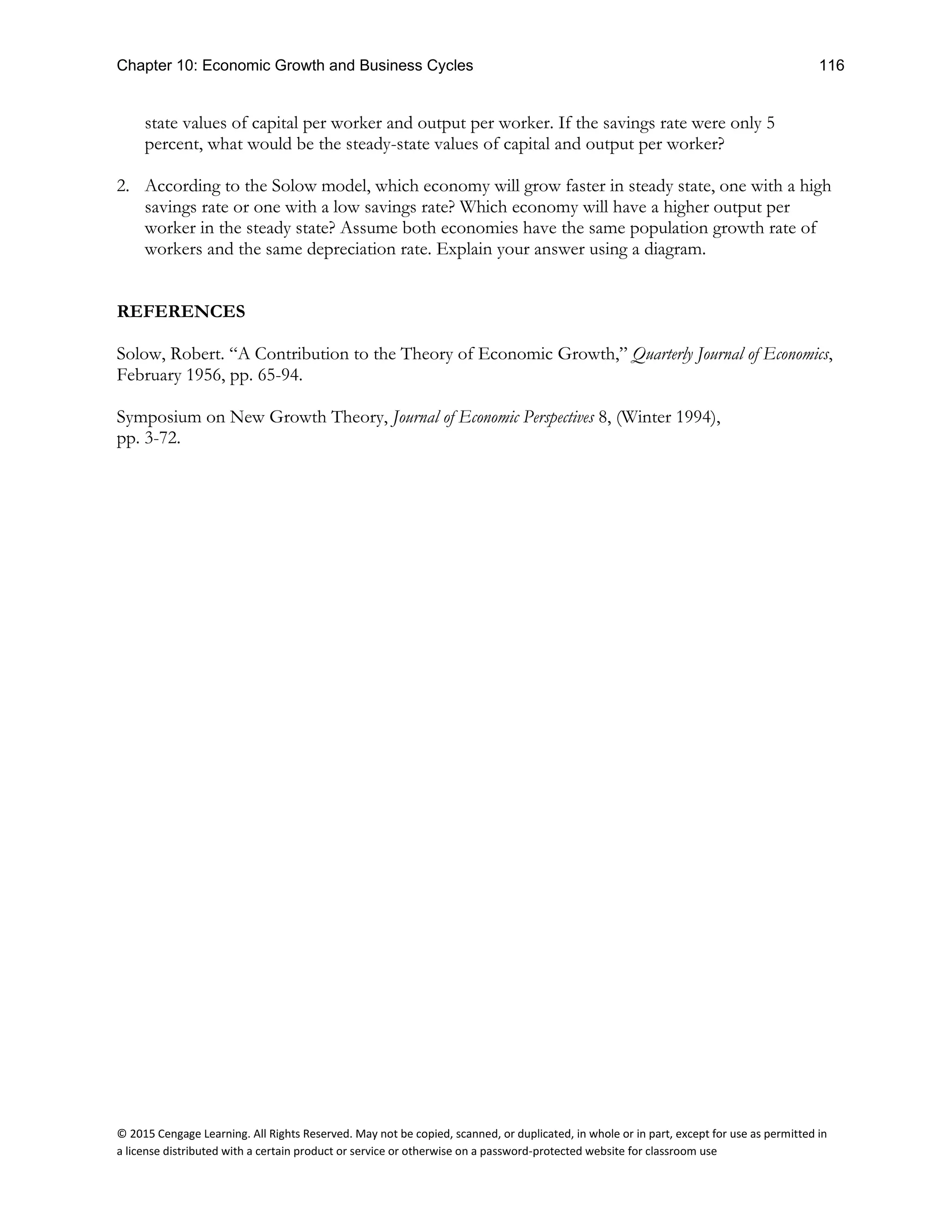
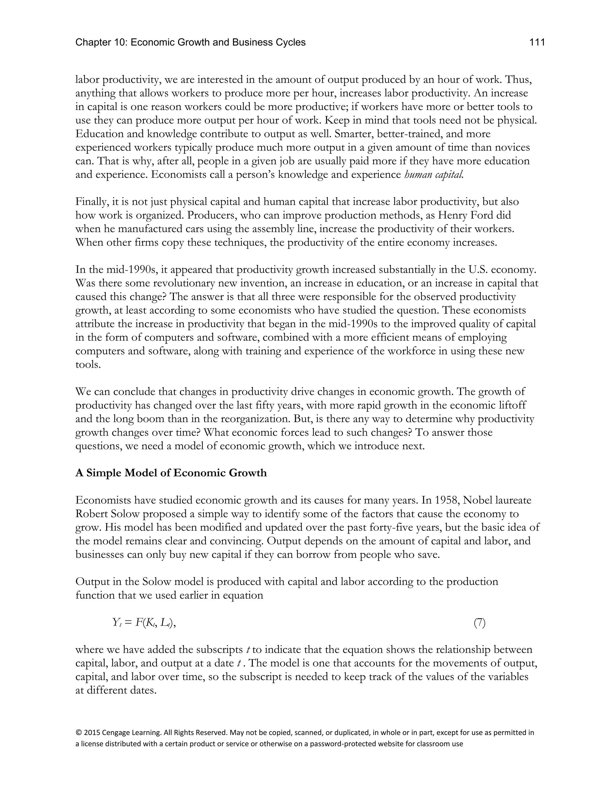
Growth of hours worked between;
1959 and 1969 =
58.88 49.15
49.15
−
= 0.198 = 19.8%
1969 and 1979 =
70.16 58.88
58.88
−
= 0.192 = 19.2%
1979 and 1989 =
83.14 70.16
70.16
−
= 0.185 = 18.5%
1989 and 1999 =
97.63 83.14
83.14
−
= 0.174 = 17.4%
1999 and 2009 =
88.36 97.63
97.63
−
= ˗0.095 = ˗ 9.5%
b. %∆ output = %∆ labor productivity + %∆ hours worked
Therefore, %∆ labor productivity = %∆ output %∆ hours worked
Therefore, 1959 to 1969 = 55.6% ˗ 19.8% = 35.8%
1969 to 1979 = 43.9% ˗ 19.2% = 24.7%
1979 to 1989 = 36.8% ˗ 18.5% = 18.3%
1989 to 1999 = 44.5% ˗ 17.4% = 27.1%
1999 to 2009 = 15.9% ˗ (˗ 9.5%) = 25.4%
c. Fastest growth in output is recorded in the 1960s, and the slowest growth in output is
recorded in the 2000s. The growth in output per hour worked is fastest in the 1960s and
slowest in the 1980s. The slow growth in output in the 2000s can be attributed to the
financial crisis of 2008 and the Great Recession. The fastest growth in output, recorded in
the 1960s, can be attributed to the Economic Liftoff.
13. From equation (4): Y = A × Ka
× L1−a
, so A = Y/( K 0.2
× L0.8
)
For 2013: A = Y/(K0.2
× L0.8
) = 10,000/(4500.2
× 5,0000.8
) = 3.2373
For 2014: A = Y/(K0.2
× L0.8
) = 10,300/(4800.2
× 5,0500.8
) = 3.2655
%ΔA = (3.2655 – 3.2373)/3.2373 = 0.87%.
14. We use the equation %ΔA = %ΔY − (a × %ΔK) − [(1 − a) × %ΔL].
In Bigcap, a = 0.3, %ΔK = 10%, %ΔL = 1%, %ΔY = 5%, so
%ΔA = %ΔY − (a × %ΔK) − [(1 − a) × %ΔL]
= 5% − (0.3 × 10%) − [(1 − 0.3) × 1%]
= 5% − 3% − 0.7%](https://image.slidesharecdn.com/17458-250704033124-a2c9edc9/75/M-and-B-3-3rd-Edition-Dean-Croushore-Solutions-Manual-9-2048.jpg)
![Chapter 10: Economic Growth and Business Cycles 110
© 2015 Cengage Learning. All Rights Reserved. May not be copied, scanned, or duplicated, in whole or in part, except for use as permitted in
a license distributed with a certain product or service or otherwise on a password-protected website for classroom use
= 1.3%.
TFP is growing fast because of much capital growth.
In Smallcap, a = 0.1, %ΔK = 3%, %ΔL = 2%, %ΔY = 4%, so
%ΔA = %ΔY − (a × %ΔK) − [(1 − a) × %ΔL]
= 4% − (0.1 × 3%) − [(1 − 0.1) × 2%]
= 4% − 0.3% − 1.8%
= 1.9%.
This economy is growing slower than Bigcap’s because capital and labor are growing more
slowly, but fast TFP growth helps economic growth.
15. If you retire at age seventy, you will have worked for forty-nine years. If your salary increases 5
percent per year, you will earn $30,000 × 1.0549
= $327,640. If your salary increases 3 percent
per year, you will earn $30,000 × 1.0349
= $127,687. This is a huge difference, which shows that
growth rates matter!
Analytical Problems
16. Per-capita growth (growth rate of output per person) matters for well-being; per-capita growth
rate = output growth rate − growth rate of population.
Country A: per-capita growth rate = 6% − 4% = 2%
Country B: per-capita growth rate = 4% − 1% = 3%
Thus, people in country B are better off because their output per person is rising faster.
17. In economic expansions:
a. Output per hour rises because labor productivity rises.
b. Hours worked per worker rises because overtime work increases.
c. Employment as a fraction of the labor force increases because more people are employed.
d. The labor force as a fraction of the population increases because people re-enter the labor
force when wages increase and jobs are plentiful.
All four of these factors cause output to grow more rapidly in expansions.
ADDITIONAL TEACHING NOTES
What Causes Productivity to Change?
Changes in productivity growth cause changes in trend output growth, so investigating the forces
driving productivity growth will help us understand the sources of output growth. In the case of](https://image.slidesharecdn.com/17458-250704033124-a2c9edc9/75/M-and-B-3-3rd-Edition-Dean-Croushore-Solutions-Manual-10-2048.jpg)
![Chapter 10: Economic Growth and Business Cycles 113
© 2015 Cengage Learning. All Rights Reserved. May not be copied, scanned, or duplicated, in whole or in part, except for use as permitted in
a license distributed with a certain product or service or otherwise on a password-protected website for classroom use
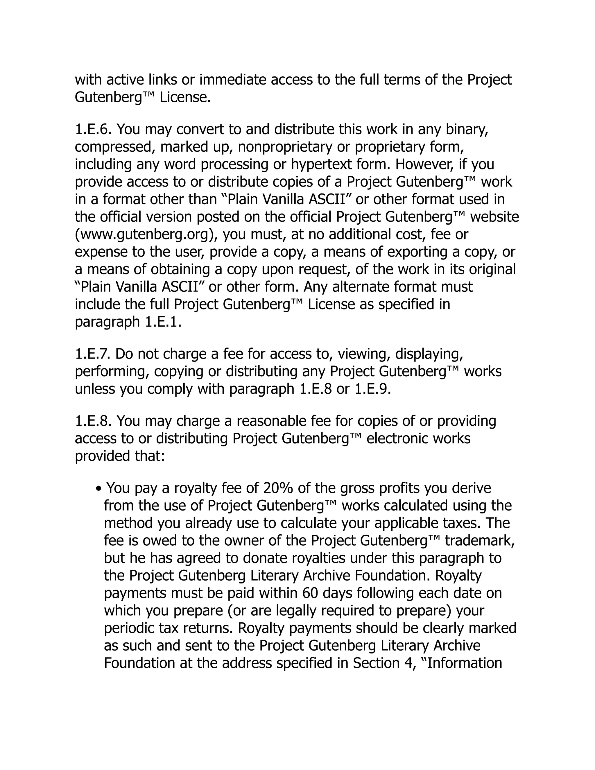
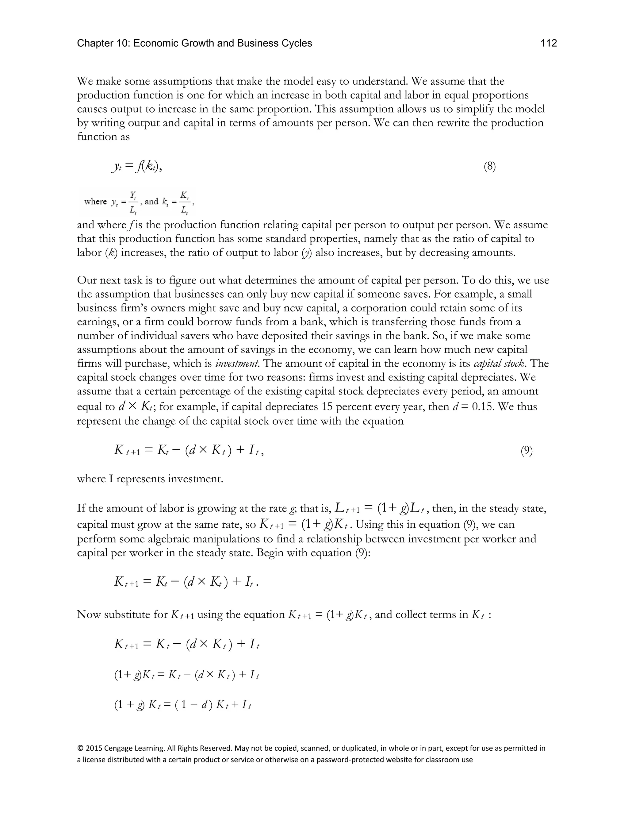
[( 1 + g ) − ( 1 − d )] K t = I t
( g + d ) K t = I t .
Now, if we switch around the two sides of the equation, then divide both sides by L t , and use the
definitions that y = Y/L and i = I/L, then we have
(10)
We make one more assumption, which is that in the long run the economy will reach a steady state,
a situation where capital, labor, and output are growing at the same rate. This means that many of
the variables that we have defined, namely those in lowercase letters that represent output per
worker, capital per worker, and investment per worker, will not change over time, so we can drop
the time subscripts in equations (8) and (10). The main equations of the model are now
y = f(k) (11)
and
i = (g + d )k . (12)
The last equation means that to keep the capital stock growing at the rate that would maintain a
constant ratio of capital to labor, investment per worker (i) must equal the growth rate of the
population plus the depreciation rate on capital times the amount of capital per worker. The first
amount (the population growth rate) reflects the investment needed to make the capital stock
increase at the same rate as population growth. The second amount (the depreciation rate)
represents the amount of investment needed to replace machinery and equipment that has worn
out.
For investment to occur, however, people must save. We will make the same assumption that
Solow did, namely, that savings per person (s) is a constant fraction (v) of output per person. That
is,
s = v × y. (13)
In this equation, v is the fraction of income that people save, and we assume it is constant over
time.
Now, if we set savings per person equal to investment per person, so s = i using equations (11) and
(12), we get](https://image.slidesharecdn.com/17458-250704033124-a2c9edc9/75/M-and-B-3-3rd-Edition-Dean-Croushore-Solutions-Manual-13-2048.jpg)