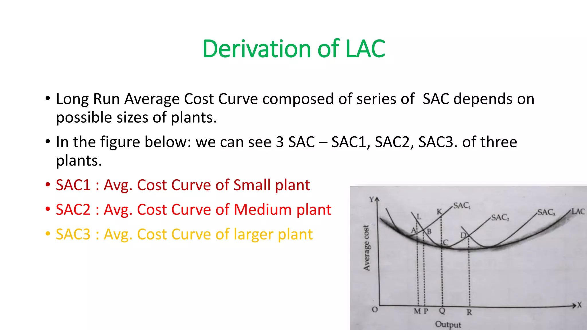
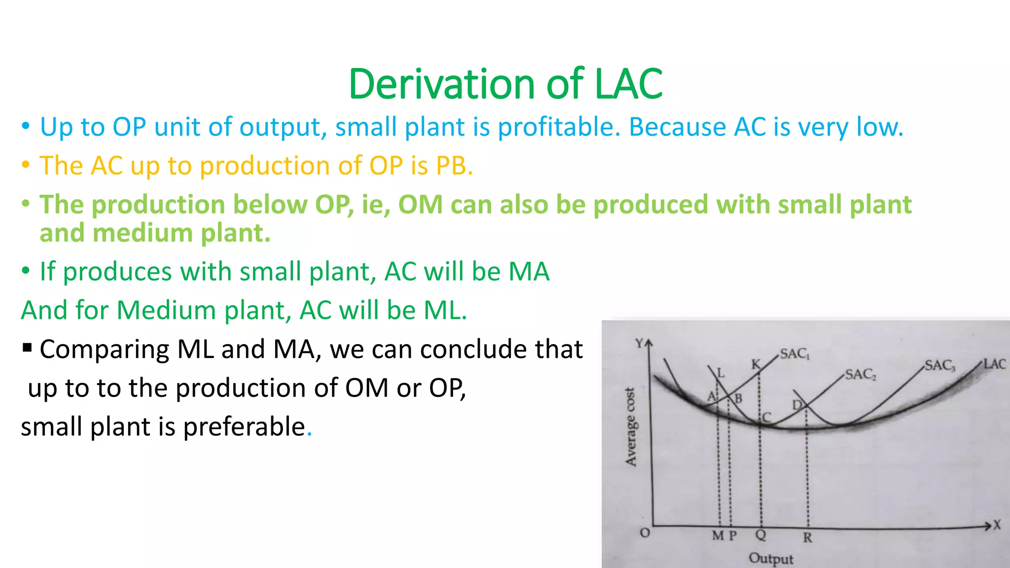
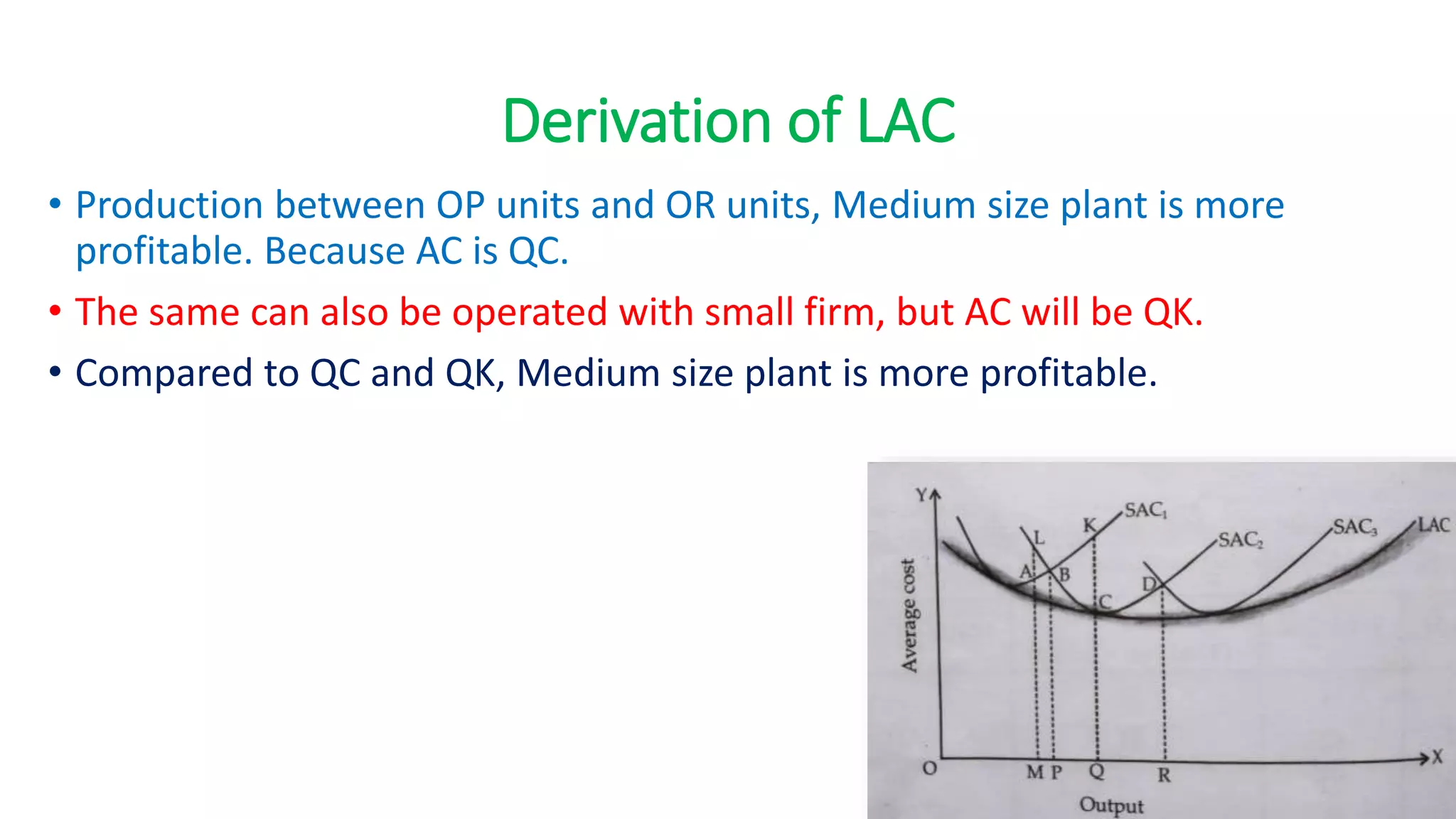
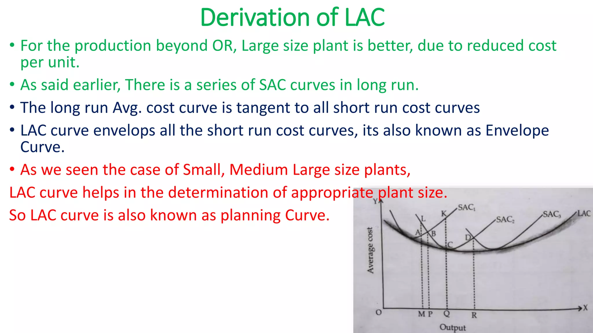
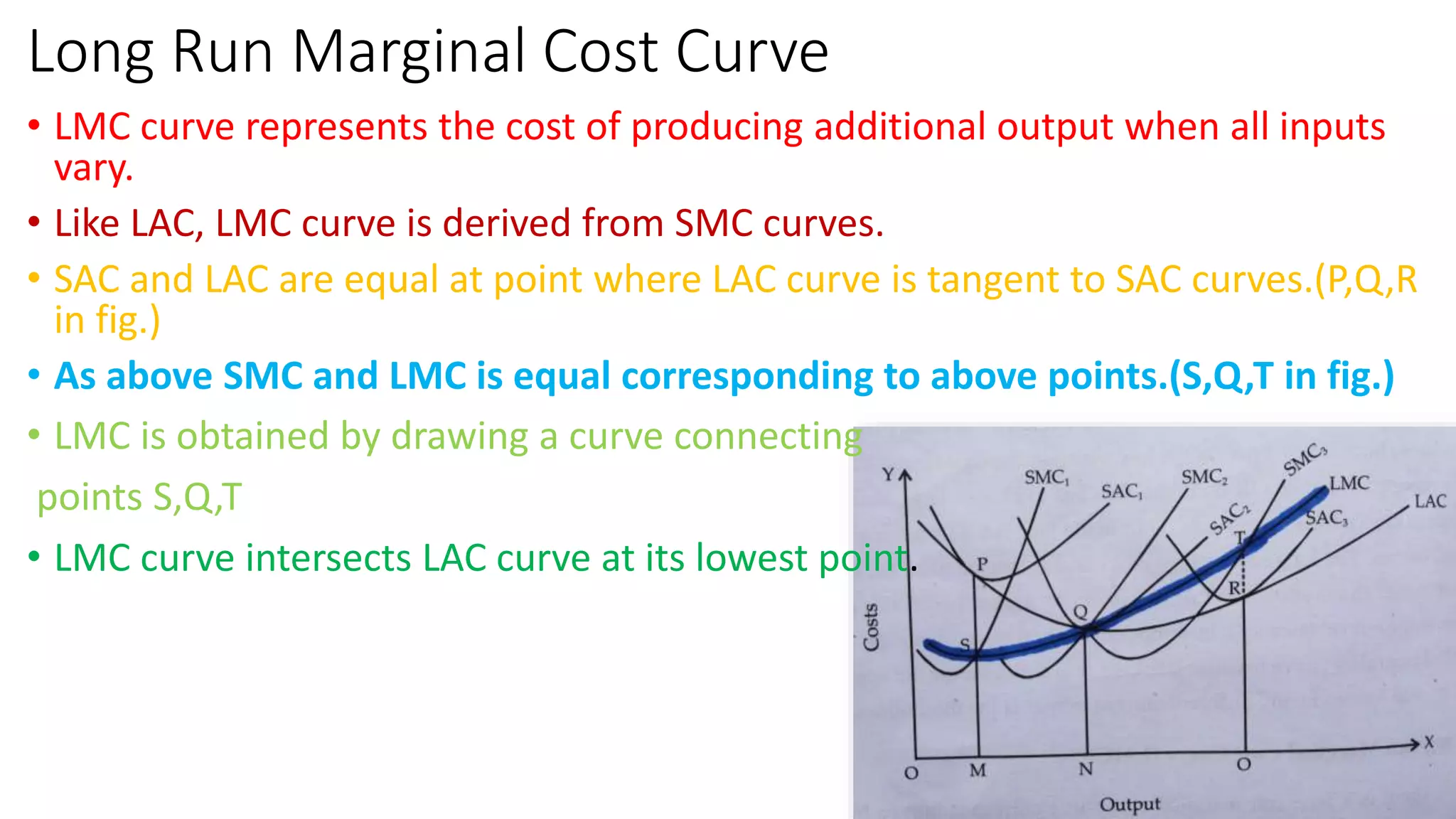
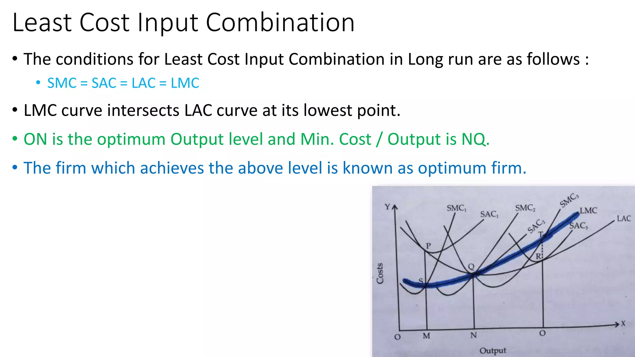
COST ANALYSIS – Part III
Long Run Cost Function
Lt.Raison Sam Raju
(M.Com, B.Ed., PGDIBO,UGC-NET-JRF,SET)
Assistant Professor in Commerce & Associate NCC Officer
Mar Thoma College, Tiruvalla
Rewind & Forward
• Determinants of Cost
• Cost Output Relationship in short run
• Long run Cost Function
• Optimum Firm
Cost Function in Long Run
• Comment the definition of Long Run.
• Features of Long Run
• No Fixed Cost
• We can increase the level of production by expanding the existing plant.
• Firms are able to expand the scale of their operation by purchasing larger quantity of all
inputs.
• In Long run all factors are variable so Cost - output relation imply the
relation between TC and Q.
• The Long Run Cost output relation is influenced by Law of Returns to
Scale.
Cost Output Function in Long Run
• In Long Run a firm can move from one plant to another.
• Firm can acquire a larger plant if want to increase output and smaller
plant if it reduces output.
• For each plant size or scale of production, the firm has separate Short
run Average Cost Curve.
• Long Run Average Cost Curve composed of series of SAC.
Derivation of LAC
• Long Run Average Cost Curve composed of series of SAC depends on
possible sizes of plants.
• In the figure below: we can see 3 SAC – SAC1, SAC2, SAC3. of three
plants.
• SAC1 : Avg. Cost Curve of Small plant
• SAC2 : Avg. Cost Curve of Medium plant
• SAC3 : Avg. Cost Curve of larger plant
Derivation of LAC
• Up to OP unit of output, small plant is profitable. Because AC is very low.
• The AC up to production of OP is PB.
• The production below OP, ie, OM can also be produced with small plant
and medium plant.
• If produces with small plant, AC will be MA
And for Medium plant, AC will be ML.
 Comparing ML and MA, we can conclude that
up to to the production of OM or OP,
small plant is preferable.
Derivation of LAC
• Production between OP units and OR units, Medium size plant is more
profitable. Because AC is QC.
• The same can also be operated with small firm, but AC will be QK.
• Compared to QC and QK, Medium size plant is more profitable.
Derivation of LAC
• For the production beyond OR, Large size plant is better, due to reduced cost
per unit.
• As said earlier, There is a series of SAC curves in long run.
• The long run Avg. cost curve is tangent to all short run cost curves
• LAC curve envelops all the short run cost curves, its also known as Envelope
Curve.
• As we seen the case of Small, Medium Large size plants,
LAC curve helps in the determination of appropriate plant size.
So LAC curve is also known as planning Curve.
Long Run Marginal Cost Curve
• LMC curve represents the cost of producing additional output when all inputs
vary.
• Like LAC, LMC curve is derived from SMC curves.
• SAC and LAC are equal at point where LAC curve is tangent to SAC curves.(P,Q,R
in fig.)
• As above SMC and LMC is equal corresponding to above points.(S,Q,T in fig.)
• LMC is obtained by drawing a curve connecting
points S,Q,T
• LMC curve intersects LAC curve at its lowest point.
Least Cost Input Combination
• The conditions for Least Cost Input Combination in Long run are as follows :
• SMC = SAC = LAC = LMC
• LMC curve intersects LAC curve at its lowest point.
• ON is the optimum Output level and Min. Cost / Output is NQ.
• The firm which achieves the above level is known as optimum firm.
Optimum Firm
• We already discussed the concept, ‘optimum firm’, both in short run
and Long Run.
• A firm reaches the optimum level of production where AC = MC.
• Maximum Productivity or Maximum efficiency point of the firm.
• At this point, the cost of production per unit will be the lowest.
• Optimum Level is not the maximum profit level.
• A firm reap its maximum profit only when its MC = MR.
Thank You
“The word Crisis is composed of two characters – one represents
danger and one represents opportunity. “ John F Kennedy.
It is that positivity we need to Cultivate right now and emerge stronger.
Be positive and stay negative to Covid19
• Stay Home….Stay Safe

Long Run Cost Function

  • 1.
    COST ANALYSIS –Part III Long Run Cost Function Lt.Raison Sam Raju (M.Com, B.Ed., PGDIBO,UGC-NET-JRF,SET) Assistant Professor in Commerce & Associate NCC Officer Mar Thoma College, Tiruvalla
  • 2.
    Rewind & Forward •Determinants of Cost • Cost Output Relationship in short run • Long run Cost Function • Optimum Firm
  • 3.
    Cost Function inLong Run • Comment the definition of Long Run. • Features of Long Run • No Fixed Cost • We can increase the level of production by expanding the existing plant. • Firms are able to expand the scale of their operation by purchasing larger quantity of all inputs. • In Long run all factors are variable so Cost - output relation imply the relation between TC and Q. • The Long Run Cost output relation is influenced by Law of Returns to Scale.
  • 4.
    Cost Output Functionin Long Run • In Long Run a firm can move from one plant to another. • Firm can acquire a larger plant if want to increase output and smaller plant if it reduces output. • For each plant size or scale of production, the firm has separate Short run Average Cost Curve. • Long Run Average Cost Curve composed of series of SAC.
  • 5.
    Derivation of LAC •Long Run Average Cost Curve composed of series of SAC depends on possible sizes of plants. • In the figure below: we can see 3 SAC – SAC1, SAC2, SAC3. of three plants. • SAC1 : Avg. Cost Curve of Small plant • SAC2 : Avg. Cost Curve of Medium plant • SAC3 : Avg. Cost Curve of larger plant
  • 6.
    Derivation of LAC •Up to OP unit of output, small plant is profitable. Because AC is very low. • The AC up to production of OP is PB. • The production below OP, ie, OM can also be produced with small plant and medium plant. • If produces with small plant, AC will be MA And for Medium plant, AC will be ML.  Comparing ML and MA, we can conclude that up to to the production of OM or OP, small plant is preferable.
  • 7.
    Derivation of LAC •Production between OP units and OR units, Medium size plant is more profitable. Because AC is QC. • The same can also be operated with small firm, but AC will be QK. • Compared to QC and QK, Medium size plant is more profitable.
  • 8.
    Derivation of LAC •For the production beyond OR, Large size plant is better, due to reduced cost per unit. • As said earlier, There is a series of SAC curves in long run. • The long run Avg. cost curve is tangent to all short run cost curves • LAC curve envelops all the short run cost curves, its also known as Envelope Curve. • As we seen the case of Small, Medium Large size plants, LAC curve helps in the determination of appropriate plant size. So LAC curve is also known as planning Curve.
  • 9.
    Long Run MarginalCost Curve • LMC curve represents the cost of producing additional output when all inputs vary. • Like LAC, LMC curve is derived from SMC curves. • SAC and LAC are equal at point where LAC curve is tangent to SAC curves.(P,Q,R in fig.) • As above SMC and LMC is equal corresponding to above points.(S,Q,T in fig.) • LMC is obtained by drawing a curve connecting points S,Q,T • LMC curve intersects LAC curve at its lowest point.
  • 10.
    Least Cost InputCombination • The conditions for Least Cost Input Combination in Long run are as follows : • SMC = SAC = LAC = LMC • LMC curve intersects LAC curve at its lowest point. • ON is the optimum Output level and Min. Cost / Output is NQ. • The firm which achieves the above level is known as optimum firm.
  • 11.
    Optimum Firm • Wealready discussed the concept, ‘optimum firm’, both in short run and Long Run. • A firm reaches the optimum level of production where AC = MC. • Maximum Productivity or Maximum efficiency point of the firm. • At this point, the cost of production per unit will be the lowest. • Optimum Level is not the maximum profit level. • A firm reap its maximum profit only when its MC = MR.
  • 12.
    Thank You “The wordCrisis is composed of two characters – one represents danger and one represents opportunity. “ John F Kennedy. It is that positivity we need to Cultivate right now and emerge stronger. Be positive and stay negative to Covid19 • Stay Home….Stay Safe