Instructor
► Dr. SanjeevKumar
Associate Professor
Department of Mathematics, IIT Roorkee
Can catch at : Room No. 302
mail at: malikfma@iitr.ac.in
gtalk: MALIKDMA@GMAIL
5.
S. No.
Contents
1. Imagefundamentals: A simple image formation model, sampling and quantization,
connectivity and adjacency relationships between pixels
2. Spatial domain filtering: Basic intensity transformations: negative, log, power-law and
piecewise linear transformations, bit-plane slicing, histogram equalization and
matching, smoothing and sharpening filtering in spatial domain, unsharp masking and
high-boost filtering
3. Frequency domain filtering: Fourier Series and Fourier transform, discrete and fast
Fourier transform, sampling theorem, aliasing, filtering in frequency domain, lowpass
and highpass filters, bandreject and bandpass filters, notch filters
4. Image restoration: Introduction to various noise models, restoration in presence of
noise only, periodic noise reduction, linear and position invariant degradation,
estimation of degradation function
5. Image reconstruction: Principles of computed tomography, projections and Radon
transform, the Fourier slice theorem, reconstruction using parallel-beam and fan-beam
by filtered backprojection methods
6. Mathematical morphology: Erosion and dilation, opening and closing, the Hit-or-Miss
transformation, various morphological algorithms for binary images
7. Wavelets and multiresolution processing: Image pyramids, subband coding,
multiresolution expansions, the Haar transform, wavelet transform in one and two
dimensions, discrete wavelet transform
6.
Gonzalez, R. C.and Woods, R. E., "Digital Image
Processing", Prentice Hall, 3rd
Ed.
Jain, A. K., "Fundamentals of Digital Image Processing",
PHI Learning, 1st
Ed.
Bernd, J., "Digital Image Processing", Springer, 6th
Ed.
Burger, W. and Burge, M. J., "Principles of Digital Image
Processing", Springer
Scherzer, O., " Handbook of Mathematical Methods in
Imaging", Springer
Weeks 1 &2
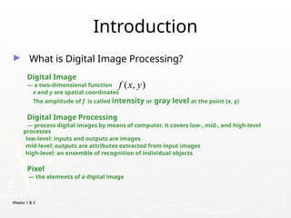
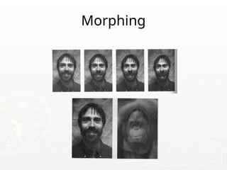
Introduction
► What is Digital Image Processing?
Digital Image
— a two-dimensional function
x and y are spatial coordinates
The amplitude of f is called intensity or gray level at the point (x, y)
Digital Image Processing
— process digital images by means of computer, it covers low-, mid-, and high-level
processes
low-level: inputs and outputs are images
mid-level: outputs are attributes extracted from input images
high-level: an ensemble of recognition of individual objects
Pixel
— the elements of a digital image
( , )
f x y
10.
Weeks 1 &2
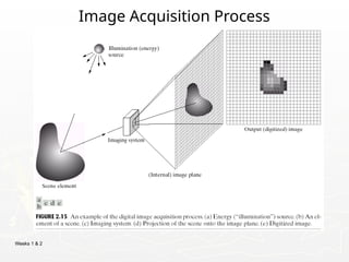
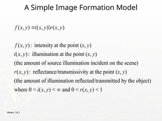
A Simple Image Formation Model
( , ) ( , ) ( , )
( , ): intensity at the point ( , )
( , ): illumination at the point ( , )
(the amount of source illumination incident on the scene)
( , ): reflectance/transmissivity
f x y i x y r x y
f x y x y
i x y x y
r x y
at the point ( , )
(the amount of illumination reflected/transmitted by the object)
where 0 < ( , ) < and 0 < ( , ) < 1
x y
i x y r x y
11.
Weeks 1 &2
Some Typical Ranges of Reflectance
► Reflectance
0.01 for black velvet
0.65 for stainless steel
0.80 for flat-white wall paint
0.90 for silver-plated metal
0.93 for snow
12.
Weeks 1 &2
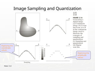
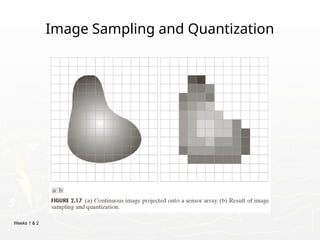
Image Sampling and Quantization
Digitizing the
coordinate
values
Digitizing the
amplitude
values
Weeks 1 &2
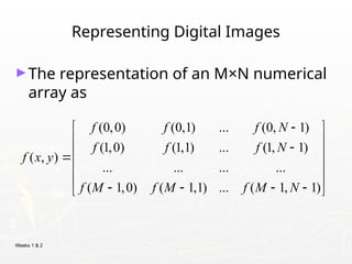
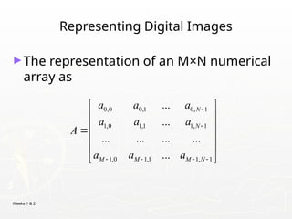
Representing Digital Images
►The representation of an M×N numerical
array as
(0,0) (0,1) ... (0, 1)
(1,0) (1,1) ... (1, 1)
( , )
... ... ... ...
( 1,0) ( 1,1) ... ( 1, 1)
f f f N
f f f N
f x y
f M f M f M N
15.
Weeks 1 &2
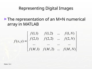
Representing Digital Images
►The representation of an M×N numerical
array as
0,0 0,1 0, 1
1,0 1,1 1, 1
1,0 1,1 1, 1
...
...
... ... ... ...
...
N
N
M M M N
a a a
a a a
A
a a a
16.
Weeks 1 &2
Representing Digital Images
►The representation of an M×N numerical
array in MATLAB
(1,1) (1,2) ... (1, )
(2,1) (2,2) ... (2, )
( , )
... ... ... ...
( ,1) ( ,2) ... ( , )
f f f N
f f f N
f x y
f M f M f M N
17.
Weeks 1 &2
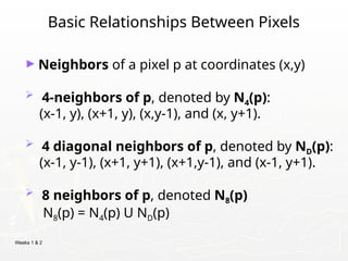
Representing Digital Images
► Discrete intensity interval [0, L-1], L=2k
► The number b of bits required to store a M × N
digitized image
b = M × N × k
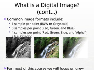
What is aDigital Image?
(cont…)
►Common image formats include:
1 sample per point (B&W or Grayscale)
3 samples per point (Red, Green, and Blue)
4 samples per point (Red, Green, Blue, and “Alpha”,
a.k.a. Opacity)
►For most of this course we will focus on grey-
23.
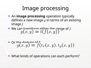
Image processing
► Animage processing operation typically
defines a new image g in terms of an existing
image f.
► We can transform either the range of f.
► Or the domain of f:
► What kinds of operations can each perform?
24.
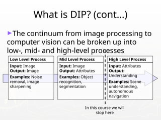
What is DIP?(cont…)
►The continuum from image processing to
computer vision can be broken up into
low-, mid- and high-level processes
Low Level Process
Input: Image
Output: Image
Examples: Noise
removal, image
sharpening
Mid Level Process
Input: Image
Output: Attributes
Examples: Object
recognition,
segmentation
High Level Process
Input: Attributes
Output:
Understanding
Examples: Scene
understanding,
autonomous
navigation
In this course we will
stop here
25.
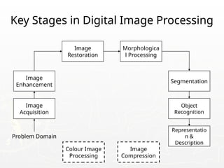
Key Stages inDigital Image Processing
Image
Acquisition
Image
Restoration
Morphologica
l Processing
Segmentation
Representatio
n &
Description
Image
Enhancement
Object
Recognition
Problem Domain
Colour Image
Processing
Image
Compression
26.
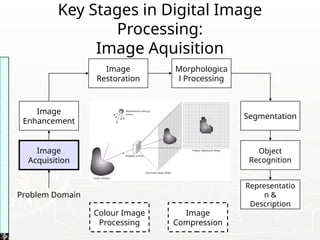
Key Stages inDigital Image
Processing:
Image Aquisition
Image
Acquisition
Image
Restoration
Morphologica
l Processing
Segmentation
Representatio
n &
Description
Image
Enhancement
Object
Recognition
Problem Domain
Colour Image
Processing
Image
Compression
Images
taken
from
Gonzalez
&
Woods,
Digital
Image
Processing
(2002)
27.
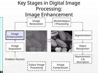
Key Stages inDigital Image
Processing:
Image Enhancement
Image
Acquisition
Image
Restoration
Morphologica
l Processing
Segmentation
Representatio
n &
Description
Image
Enhancement
Object
Recognition
Problem Domain
Colour Image
Processing
Image
Compression
Images
taken
from
Gonzalez
&
Woods,
Digital
Image
Processing
(2002)
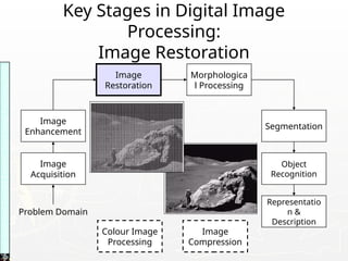
28.
Key Stages inDigital Image
Processing:
Image Restoration
Image
Acquisition
Image
Restoration
Morphologica
l Processing
Segmentation
Representatio
n &
Description
Image
Enhancement
Object
Recognition
Problem Domain
Colour Image
Processing
Image
Compression
Images
taken
from
Gonzalez
&
Woods,
Digital
Image
Processing
(2002)
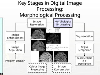
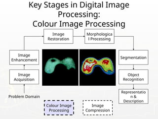
29.
Key Stages inDigital Image
Processing:
Morphological Processing
Image
Acquisition
Image
Restoration
Morphologica
l Processing
Segmentation
Representatio
n &
Description
Image
Enhancement
Object
Recognition
Problem Domain
Colour Image
Processing
Image
Compression
Images
taken
from
Gonzalez
&
Woods,
Digital
Image
Processing
(2002)
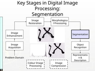
30.
Key Stages inDigital Image
Processing:
Segmentation
Image
Acquisition
Image
Restoration
Morphologica
l Processing
Segmentation
Representatio
n &
Description
Image
Enhancement
Object
Recognition
Problem Domain
Colour Image
Processing
Image
Compression
Images
taken
from
Gonzalez
&
Woods,
Digital
Image
Processing
(2002)
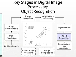
31.
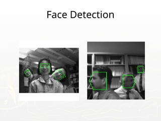
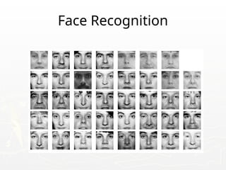
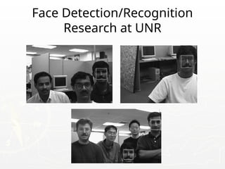
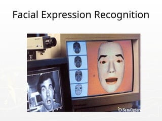
Key Stages inDigital Image
Processing:
Object Recognition
Image
Acquisition
Image
Restoration
Morphologica
l Processing
Segmentation
Representatio
n &
Description
Image
Enhancement
Object
Recognition
Problem Domain
Colour Image
Processing
Image
Compression
Images
taken
from
Gonzalez
&
Woods,
Digital
Image
Processing
(2002)
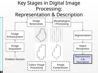
32.
Key Stages inDigital Image
Processing:
Representation & Description
Image
Acquisition
Image
Restoration
Morphologica
l Processing
Segmentation
Representatio
n &
Description
Image
Enhancement
Object
Recognition
Problem Domain
Colour Image
Processing
Image
Compression
Images
taken
from
Gonzalez
&
Woods,
Digital
Image
Processing
(2002)
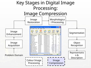
33.
Key Stages inDigital Image
Processing:
Image Compression
Image
Acquisition
Image
Restoration
Morphologica
l Processing
Segmentation
Representatio
n &
Description
Image
Enhancement
Object
Recognition
Problem Domain
Colour Image
Processing
Image
Compression
Companies In thisField In India
► Sarnoff Corporation
► Kritikal Solutions
► National Instruments
► GE Laboratories
► Ittiam, Bangalore
► Interra Systems, Noida
► Yahoo India (Multimedia Searching)
► nVidia Graphics, Pune (have high requirements)
► Microsoft research
► DRDO labs
► ISRO labs
► …
Weeks 1 &2
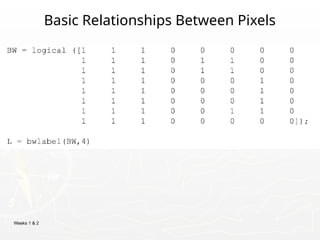
Basic Relationships Between Pixels
► Neighborhood
► Adjacency
► Connectivity
► Paths
► Regions and boundaries
63.
Weeks 1 &2
Basic Relationships Between Pixels
► Neighbors of a pixel p at coordinates (x,y)
4-neighbors of p, denoted by N4(p):
(x-1, y), (x+1, y), (x,y-1), and (x, y+1).
4 diagonal neighbors of p, denoted by ND(p):
(x-1, y-1), (x+1, y+1), (x+1,y-1), and (x-1, y+1).
8 neighbors of p, denoted N8(p)
N8(p) = N4(p) U ND(p)
64.
Weeks 1 &2
Basic Relationships Between Pixels
► Adjacency
Let V be the set of intensity values
4-adjacency: Two pixels p and q with values from V are
4-adjacent if q is in the set N4(p).
8-adjacency: Two pixels p and q with values from V are
8-adjacent if q is in the set N8(p).
65.
Weeks 1 &2
Basic Relationships Between Pixels
► Adjacency
Let V be the set of intensity values
m-adjacency: Two pixels p and q with values from V are
m-adjacent if
(i) q is in the set N4(p), or
(ii) q is in the set ND(p) and the set N4(p) ∩ N4(p) has no pixels whose
values are from V.
66.
Weeks 1 &2
Basic Relationships Between Pixels
► Path
A (digital) path (or curve) from pixel p with coordinates (x0, y0) to
pixel q with coordinates (xn, yn) is a sequence of distinct pixels with
coordinates
(x0, y0), (x1, y1), …, (xn, yn)
Where (xi, yi) and (xi-1, yi-1) are adjacent for 1 i n.
≤ ≤
Here n is the length of the path.
If (x0, y0) = (xn, yn), the path is closed path.
We can define 4-, 8-, and m-paths based on the type of adjacency
used.
Weeks 1 &2
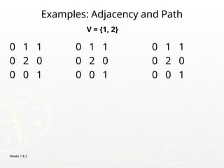
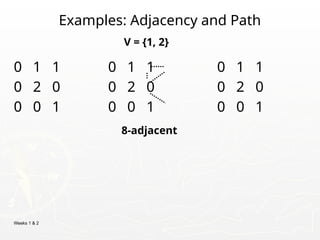
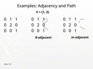
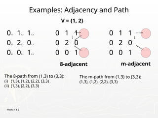
Examples: Adjacency and Path
01,1 11,2 11,3 0 1 1 0 1 1
02,1 22,2 02,3 0 2 0 0 2 0
03,1 03,2 13,3 0 0 1 0 0 1
V = {1, 2}
8-adjacent m-adjacent
The 8-path from (1,3) to (3,3):
(i) (1,3), (1,2), (2,2), (3,3)
(ii) (1,3), (2,2), (3,3)
The m-path from (1,3) to (3,3):
(1,3), (1,2), (2,2), (3,3)
71.
Weeks 1 &2
Basic Relationships Between Pixels
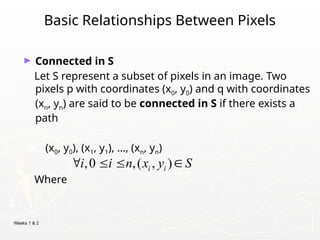
► Connected in S
Let S represent a subset of pixels in an image. Two
pixels p with coordinates (x0, y0) and q with coordinates
(xn, yn) are said to be connected in S if there exists a
path
(x0, y0), (x1, y1), …, (xn, yn)
Where
,0 ,( , )
i i
i i n x y S
72.
Weeks 1 &2
Basic Relationships Between Pixels
Let S represent a subset of pixels in an image
► For every pixel p in S, the set of pixels in S that are connected to p
is called a connected component of S.
► If S has only one connected component, then S is called Connected
Set.
► We call R a region of the image if R is a connected set
► Two regions, Ri and Rj are said to be adjacent if their union forms a
connected set.
► Regions that are not to be adjacent are said to be disjoint.
Weeks 1 &2
Basic Relationships Between Pixels
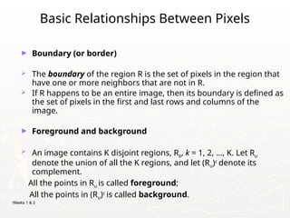
► Boundary (or border)
The boundary of the region R is the set of pixels in the region that
have one or more neighbors that are not in R.
If R happens to be an entire image, then its boundary is defined as
the set of pixels in the first and last rows and columns of the
image.
► Foreground and background
An image contains K disjoint regions, Rk, k = 1, 2, …, K. Let Ru
denote the union of all the K regions, and let (Ru)c
denote its
complement.
All the points in Ru is called foreground;
All the points in (Ru)c
is called background.
78.
Weeks 1 &2
Question 1
► In the following arrangement of pixels, are the two
regions (of 1s) adjacent? (if 8-adjacency is used)
1 1 1
1 0 1
0 1 0
0 0 1
1 1 1
1 1 1
Region 1
Region 2
79.
Weeks 1 &2
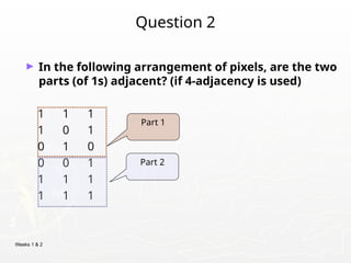
Question 2
► In the following arrangement of pixels, are the two
parts (of 1s) adjacent? (if 4-adjacency is used)
1 1 1
1 0 1
0 1 0
0 0 1
1 1 1
1 1 1
Part 1
Part 2
80.
Weeks 1 &2
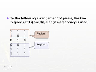
► In the following arrangement of pixels, the two
regions (of 1s) are disjoint (if 4-adjacency is used)
1 1 1
1 0 1
0 1 0
0 0 1
1 1 1
1 1 1
Region 1
Region 2
81.
Weeks 1 &2
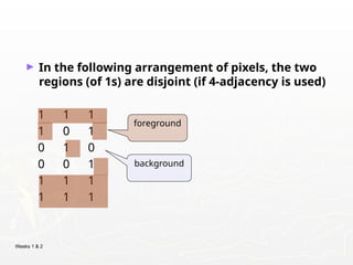
► In the following arrangement of pixels, the two
regions (of 1s) are disjoint (if 4-adjacency is used)
1 1 1
1 0 1
0 1 0
0 0 1
1 1 1
1 1 1
foreground
background
82.
Weeks 1 &2
Question 3
► In the following arrangement of pixels, the circled
point is part of the boundary of the 1-valued pixels if
8-adjacency is used, true or false?
0 0 0 0 0
0 1 1 0 0
0 1 1 0 0
0 1 1 1 0
0 1 1 1 0
0 0 0 0 0
83.
Weeks 1 &2
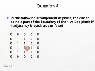
Question 4
► In the following arrangement of pixels, the circled
point is part of the boundary of the 1-valued pixels if
4-adjacency is used, true or false?
0 0 0 0 0
0 1 1 0 0
0 1 1 0 0
0 1 1 1 0
0 1 1 1 0
0 0 0 0 0
84.
Weeks 1 &2
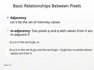
Distance Measures
► Given pixels p, q and z with coordinates (x, y), (s, t),
(u, v) respectively, the distance function D has
following properties:
a. D(p, q) 0 [D(p, q) = 0, iff p = q]
≥
b. D(p, q) = D(q, p)
c. D(p, z) D(p, q) + D(q, z)
≤
85.
Weeks 1 &2
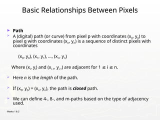
Distance Measures
The following are the different Distance measures:
a. Euclidean Distance :
De(p, q) = [(x-s)2
+ (y-t)2
]1/2
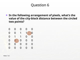
b. City Block Distance:
D4(p, q) = |x-s| + |y-t|
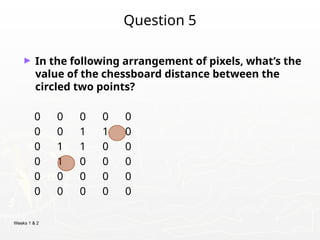
c. Chess Board Distance:
D8(p, q) = max(|x-s|, |y-t|)
86.
Weeks 1 &2
Question 5
► In the following arrangement of pixels, what’s the
value of the chessboard distance between the
circled two points?
0 0 0 0 0
0 0 1 1 0
0 1 1 0 0
0 1 0 0 0
0 0 0 0 0
0 0 0 0 0
87.
Weeks 1 &2
Question 6
► In the following arrangement of pixels, what’s the
value of the city-block distance between the circled
two points?
0 0 0 0 0
0 0 1 1 0
0 1 1 0 0
0 1 0 0 0
0 0 0 0 0
0 0 0 0 0
88.
Weeks 1 &2
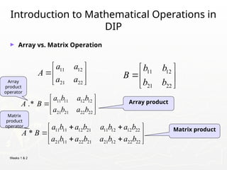
Introduction to Mathematical Operations in
DIP
► Array vs. Matrix Operation
11 12
21 22
b b
B
b b
11 12
21 22
a a
A
a a
11 11 12 21 11 12 12 22
21 11 22 21 21 12 22 22
*
a b a b a b a b
A B
a b a b a b a b
11 11 12 12
21 21 22 22
.*
a b a b
A B
a b a b
Array product
Matrix product
Array
product
operator
Matrix
product
operator
89.
Weeks 1 &2
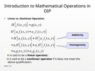
Introduction to Mathematical Operations in
DIP
► Linear vs. Nonlinear Operation
H is said to be a linear operator;
H is said to be a nonlinear operator if it does not meet the
above qualification.
( , ) ( , )
H f x y g x y
Additivity
Homogeneity
( , ) ( , )
( , ) ( , )
( , ) ( , )
( , ) ( , )
i i j j
i i j j
i i j j
i i j j
H a f x y a f x y
H a f x y H a f x y
a H f x y a H f x y
a g x y a g x y
90.
Weeks 1 &2
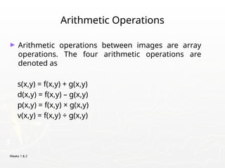
Arithmetic Operations
► Arithmetic operations between images are array
operations. The four arithmetic operations are
denoted as
s(x,y) = f(x,y) + g(x,y)
d(x,y) = f(x,y) – g(x,y)
p(x,y) = f(x,y) × g(x,y)
v(x,y) = f(x,y) ÷ g(x,y)
91.
Weeks 1 &2
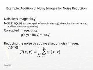
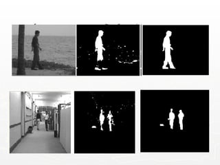
Example: Addition of Noisy Images for Noise Reduction
Noiseless image: f(x,y)
Noise: n(x,y) (at every pair of coordinates (x,y), the noise is uncorrelated
and has zero average value)
Corrupted image: g(x,y)
g(x,y) = f(x,y) + n(x,y)
Reducing the noise by adding a set of noisy images,
{gi(x,y)}
1
1
( , ) ( , )
K
i
i
g x y g x y
K
92.
Weeks 1 &2
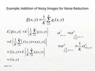
Example: Addition of Noisy Images for Noise Reduction
1
1
1
1
( , ) ( , )
1
( , ) ( , )
1
( , ) ( , )
( , )
K
i
i
K
i
i
K
i
i
E g x y E g x y
K
E f x y n x y
K
f x y E n x y
K
f x y
1
1
( , ) ( , )
K
i
i
g x y g x y
K
2
( , ) 1
( , )
1
1
( , )
1
2
2 2
( , )
1
g x y K
g x y
i
K i
K
n x y
i
K i
n x y
K
93.
Weeks 1 &2
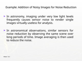
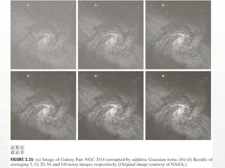
Example: Addition of Noisy Images for Noise Reduction
► In astronomy, imaging under very low light levels
frequently causes sensor noise to render single
images virtually useless for analysis.
► In astronomical observations, similar sensors for
noise reduction by observing the same scene over
long periods of time. Image averaging is then used
to reduce the noise.
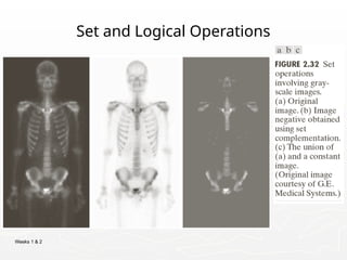
Weeks 1 &2
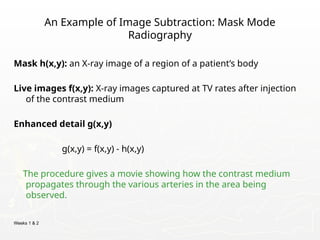
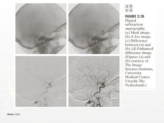
An Example of Image Subtraction: Mask Mode
Radiography
Mask h(x,y): an X-ray image of a region of a patient’s body
Live images f(x,y): X-ray images captured at TV rates after injection
of the contrast medium
Enhanced detail g(x,y)
g(x,y) = f(x,y) - h(x,y)
The procedure gives a movie showing how the contrast medium
propagates through the various arteries in the area being
observed.
Weeks 1 &2
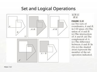
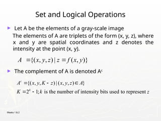
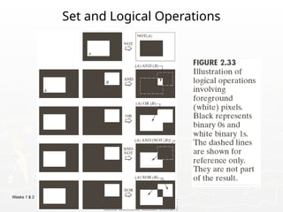
Set and Logical Operations
► Let A be the elements of a gray-scale image
The elements of A are triplets of the form (x, y, z), where
x and y are spatial coordinates and z denotes the
intensity at the point (x, y).
► The complement of A is denoted Ac
{( , , ) | ( , , ) }
2 1; is the number of intensity bits used to represent
c
k
A x y K z x y z A
K k z
{( , , ) | ( , )}
A x y z z f x y
100.
Weeks 1 &2
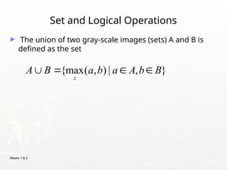
Set and Logical Operations
► The union of two gray-scale images (sets) A and B is
defined as the set
{max( , ) | , }
z
A B a b a A b B
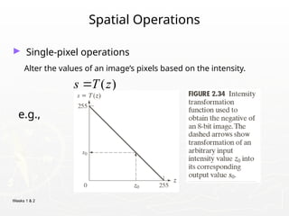
Weeks 1 &2
Spatial Operations
► Single-pixel operations
Alter the values of an image’s pixels based on the intensity.
e.g.,
( )
s T z
104.
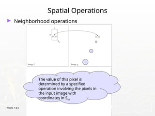
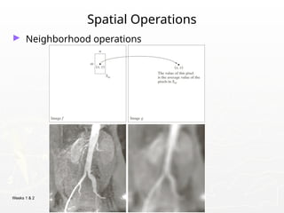
Weeks 1 &2
Spatial Operations
► Neighborhood operations
The value of this pixel is
determined by a specified
operation involving the pixels in
the input image with
coordinates in Sxy
Weeks 1 &2
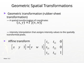
Geometric Spatial Transformations
► Geometric transformation (rubber-sheet
transformation)
— A spatial transformation of coordinates
— intensity interpolation that assigns intensity values to the spatially
transformed pixels.
► Affine transform
( , ) {( , )}
x y T v w
11 12
21 22
31 32
0
1 1 0
1
t t
x y v w t t
t t
Weeks 1 &2
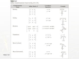
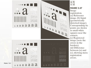
Image Registration
► Input and output images are available but the
transformation function is unknown.
Goal: estimate the transformation function and use it to
register the two images.
► One of the principal approaches for image registration
is to use tie points (also called control points)
The corresponding points are known precisely in the
input and output (reference) images.
109.
Weeks 1 &2
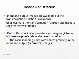
Image Registration
► A simple model based on bilinear approximation:
1 2 3 4
5 6 7 8
Where ( , ) and ( , ) are the coordinates of
tie points in the input and reference images.
x c v c w c vw c
y c v c w c vw c
v w x y
Weeks 1 &2
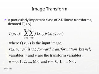
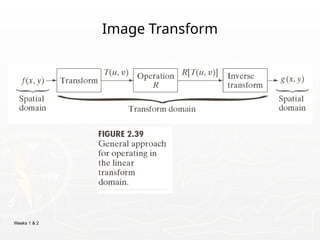
Image Transform
► A particularly important class of 2-D linear transforms,
denoted T(u, v)
1 1
0 0
( , ) ( , ) ( , , , )
where ( , ) is the input image,
( , , , ) is the ker ,
variables and are the transform variables,
= 0, 1, 2, ..., M-1 and = 0, 1,
M N
x y
T u v f x y r x y u v
f x y
r x y u v forward transformation nel
u v
u v
..., N-1.
112.
Weeks 1 &2
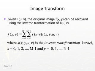
Image Transform
► Given T(u, v), the original image f(x, y) can be recoverd
using the inverse tranformation of T(u, v).
1 1
0 0
( , ) ( , ) ( , , , )
where ( , , , ) is the ker ,
= 0, 1, 2, ..., M-1 and = 0, 1, ..., N-1.
M N
u v
f x y T u v s x y u v
s x y u v inverse transformation nel
x y
Weeks 1 &2
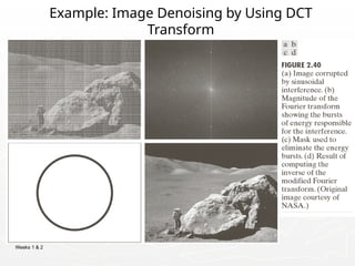
Example: Image Denoising by Using DCT
Transform
115.
Weeks 1 &2
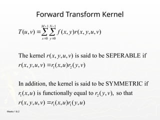
Forward Transform Kernel
1 1
0 0
1 2
1 2
( , ) ( , ) ( , , , )
The kernel ( , , , ) is said to be SEPERABLE if
( , , , ) ( , ) ( , )
In addition, the kernel is said to be SYMMETRIC if
( , ) is functionally equal to ( ,
M N
x y
T u v f x y r x y u v
r x y u v
r x y u v r x u r y v
r x u r y v
1 1
), so that
( , , , ) ( , ) ( , )
r x y u v r x u r y u
116.
Weeks 1 &2
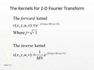
The Kernels for 2-D Fourier Transform
2 ( / / )
2 ( / / )
The kernel
( , , , )
Where = 1
The kernel
1
( , , , )
j ux M vy N
j ux M vy N
forward
r x y u v e
j
inverse
s x y u v e
MN
117.
Weeks 1 &2
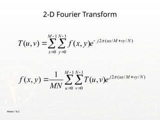
2-D Fourier Transform
1 1
2 ( / / )
0 0
1 1
2 ( / / )
0 0
( , ) ( , )
1
( , ) ( , )
M N
j ux M vy N
x y
M N
j ux M vy N
u v
T u v f x y e
f x y T u v e
MN
118.
Weeks 1 &2
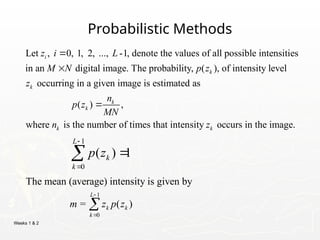
Probabilistic Methods
Let , 0, 1, 2, ..., -1, denote the values of all possible intensities
in an digital image. The probability, ( ), of intensity level
occurring in a given image is estimated as
i
k
k
z i L
M N p z
z
( ) ,
where is the number of times that intensity occurs in the image.
k
k
k k
n
p z
MN
n z
1
0
( ) 1
L
k
k
p z
1
0
The mean (average) intensity is given by
= ( )
L
k k
k
m z p z
119.
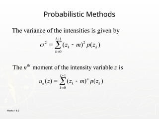
Weeks 1 &2
Probabilistic Methods
1
2 2
0
The variance of the intensities is given by
= ( ) ( )
L
k k
k
z m p z
th
1
0
The moment of the intensity variable is
( ) = ( ) ( )
L
n
n k k
k
n z
u z z m p z
120.
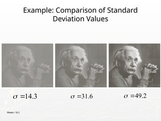
Weeks 1 &2
Example: Comparison of Standard
Deviation Values
31.6
14.3
49.2
#24 Give the analogy of the character recognition system.
Low Level: Cleaning up the image of some text
Mid level: Segmenting the text from the background and recognising individual characters
High level: Understanding what the text says


![Weeks 1 & 2
Representing Digital Images
► Discrete intensity interval [0, L-1], L=2k
► The number b of bits required to store a M × N
digitized image
b = M × N × k](https://image.slidesharecdn.com/lectures1-3final-250421174718-5478c36f/85/Lectures-on-digital-image-processing-1-3-final-pptx-17-320.jpg)


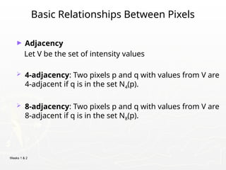
![Weeks 1 & 2
Basic Relationships Between Pixels
BW = imread('text.png');
imshow(BW);
CC = bwconncomp(BW);
numPixels =
cellfun(@numel,CC.PixelIdxList);
[biggest,idx] = max(numPixels);
BW(CC.PixelIdxList{idx}) = 0;
figure, imshow(BW);](https://image.slidesharecdn.com/lectures1-3final-250421174718-5478c36f/85/Lectures-on-digital-image-processing-1-3-final-pptx-76-320.jpg)


![Weeks 1 & 2
Distance Measures
► Given pixels p, q and z with coordinates (x, y), (s, t),
(u, v) respectively, the distance function D has
following properties:
a. D(p, q) 0 [D(p, q) = 0, iff p = q]
≥
b. D(p, q) = D(q, p)
c. D(p, z) D(p, q) + D(q, z)
≤](https://image.slidesharecdn.com/lectures1-3final-250421174718-5478c36f/85/Lectures-on-digital-image-processing-1-3-final-pptx-84-320.jpg)
![Weeks 1 & 2
Distance Measures
The following are the different Distance measures:
a. Euclidean Distance :
De(p, q) = [(x-s)2
+ (y-t)2
]1/2
b. City Block Distance:
D4(p, q) = |x-s| + |y-t|
c. Chess Board Distance:
D8(p, q) = max(|x-s|, |y-t|)](https://image.slidesharecdn.com/lectures1-3final-250421174718-5478c36f/85/Lectures-on-digital-image-processing-1-3-final-pptx-85-320.jpg)