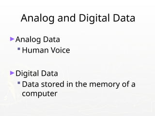
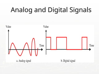
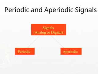
The document outlines the educational background and research interests of Muhammad Tahir Mumtaz, focusing on topics such as signal processing, digital image processing, and the differences between analog and digital data. It discusses the concepts of periodic and aperiodic signals, digital signal processing techniques, and the function of analog-to-digital and digital-to-analog converters. Additionally, it covers the fundamentals of image representation, image interpolation, and basic pixel relationships in digital image processing.


![. 90
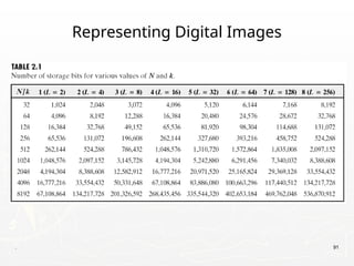
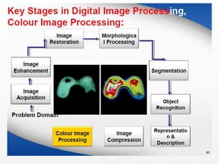
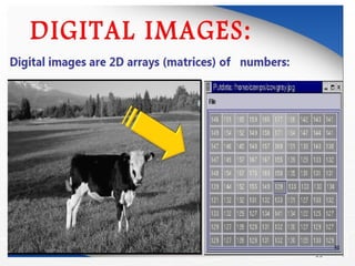
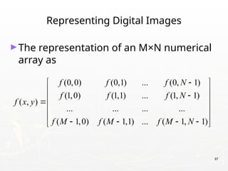
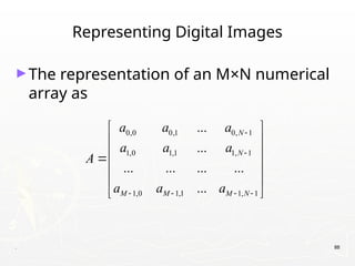
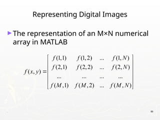
Representing Digital Images
► Discrete intensity interval [0, L-1], L=2k
► The number b of bits required to store a M × N
digitized image
b = M × N × k](https://image.slidesharecdn.com/diplecture1-8-240802061158-d6445230/85/DIP-Lecture-1-8-Digital-Image-Processing-Presentation-pptx-90-320.jpg)