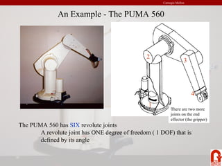
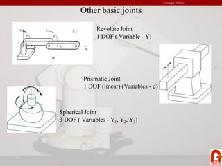
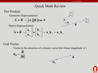
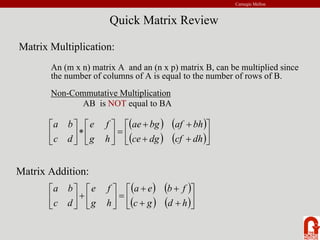
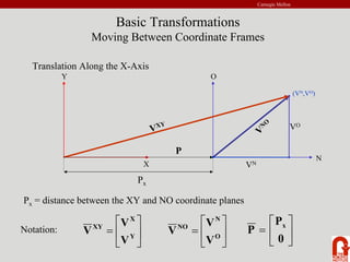
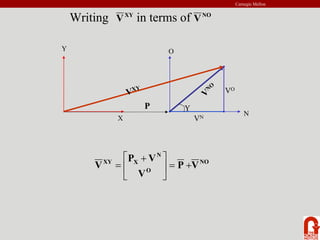
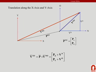
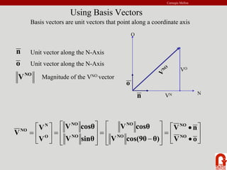
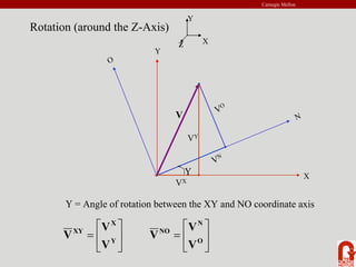
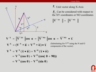
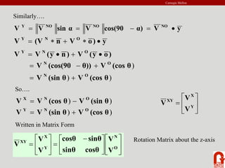
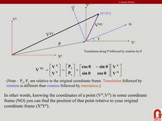
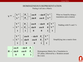
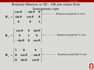
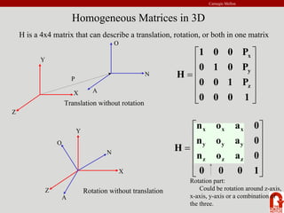
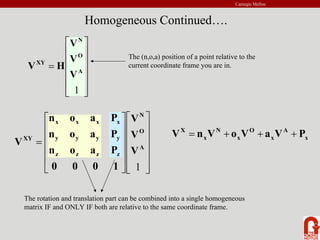
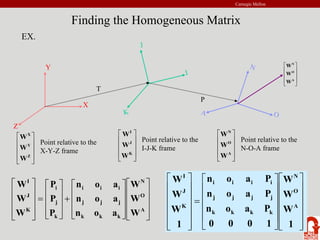
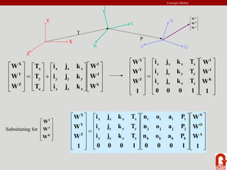
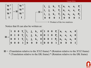
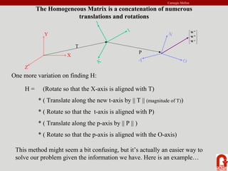
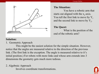
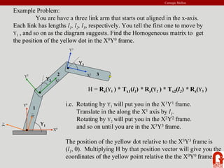
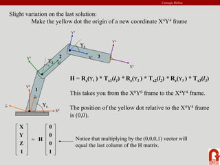
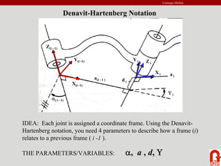
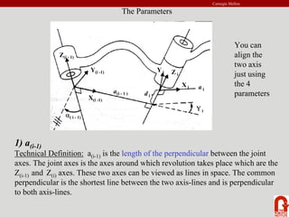
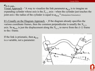
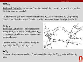
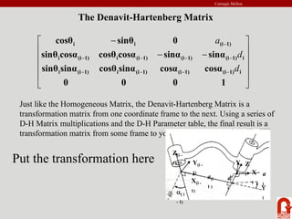
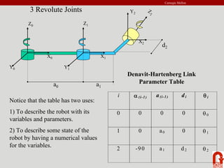
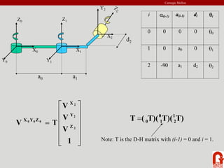
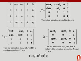
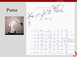
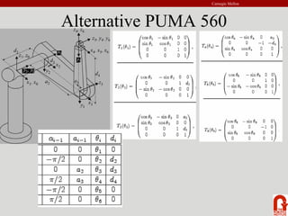
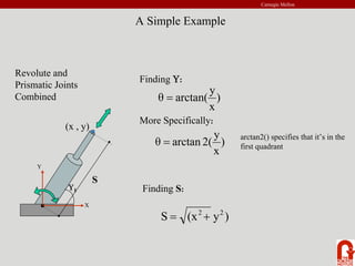
Carnegie Mellon
An Introduction to
Robot Kinematics
Renata Melamud
Carnegie Mellon
An Example - The PUMA 560
The PUMA 560 has SIX revolute joints
A revolute joint has ONE degree of freedom ( 1 DOF) that is
defined by its angle
1
2
3
4
There are two more
joints on the end
effector (the gripper)
Carnegie Mellon
Other basic joints
Spherical Joint
3 DOF ( Variables - Υ1, Υ2, Υ3)
Revolute Joint
1 DOF ( Variable - Υ)
Prismatic Joint
1 DOF (linear) (Variables - d)
Carnegie Mellon
We are interested in two kinematics topics
Forward Kinematics (angles to position)
What you are given: The length of each link
The angle of each joint
What you can find: The position of any point
(i.e. it’s (x, y, z) coordinates
Inverse Kinematics (position to angles)
What you are given: The length of each link
The position of some point on the robot
What you can find: The angles of each joint needed to obtain
that position
Carnegie Mellon
Quick Math Review
Dot Product:
Geometric Representation:
A
B
θ
cos θ
B
A
B
A =
•
Unit Vector
Vector in the direction of a chosen vector but whose magnitude is 1.
B
B
uB =
⎥
⎦
⎤
⎢
⎣
⎡
y
x
a
a
Matrix Representation:
⎥
⎦
⎤
⎢
⎣
⎡
y
x
b
b
y
y
x
x
y
x
y
x
b
a
b
a
b
b
a
a
B
A +
=
⎥
⎦
⎤
⎢
⎣
⎡
•
⎥
⎦
⎤
⎢
⎣
⎡
=
•
B
B
u
Carnegie Mellon
Quick Matrix Review
Matrix Multiplication:
An (m x n) matrix A and an (n x p) matrix B, can be multiplied since
the number of columns of A is equal to the number of rows of B.
Non-Commutative Multiplication
AB is NOT equal to BA
( ) ( )
( ) ( )⎥
⎦
⎤
⎢
⎣
⎡
+
+
+
+
=
⎥
⎦
⎤
⎢
⎣
⎡
∗
⎥
⎦
⎤
⎢
⎣
⎡
dh
cf
dg
ce
bh
af
bg
ae
h
g
f
e
d
c
b
a
Matrix Addition:
( ) ( )
( ) ( )⎥
⎦
⎤
⎢
⎣
⎡
+
+
+
+
=
⎥
⎦
⎤
⎢
⎣
⎡
+
⎥
⎦
⎤
⎢
⎣
⎡
h
d
g
c
f
b
e
a
h
g
f
e
d
c
b
a
Carnegie Mellon
Basic Transformations
Moving Between Coordinate Frames
Translation Along the X-Axis
N
O
Y
V
NO
VXY
X
Px
VN
VO
Px = distance between the XY and NO coordinate planes
⎥
⎦
⎤
⎢
⎣
⎡
= Y
X
XY
V
V
V ⎥
⎦
⎤
⎢
⎣
⎡
= O
N
NO
V
V
V ⎥
⎦
⎤
⎢
⎣
⎡
=
0
P
P x
P
(VN,VO)
Notation:
Carnegie Mellon
N
X
V
NO
VXY
P
VN
VO
O
Y
Υ
NO
O
N
X
XY
V
P
V
V
P
V +
=
⎥
⎦
⎤
⎢
⎣
⎡ +
=
Writing in terms of
XY
V NO
V
Carnegie Mellon
X
VXY
PXY
N
V
NO
VN
VO
Y
O
Translation along the X-Axis and Y-Axis
⎥
⎦
⎤
⎢
⎣
⎡
+
+
=
+
= O
Y
N
X
NO
XY
V
P
V
P
V
P
V
⎥
⎦
⎤
⎢
⎣
⎡
=
Y
x
XY
P
P
P
Carnegie Mellon
⎥
⎦
⎤
⎢
⎣
⎡
•
•
=
⎥
⎥
⎦
⎤
⎢
⎢
⎣
⎡
−
=
⎥
⎥
⎦
⎤
⎢
⎢
⎣
⎡
=
⎥
⎦
⎤
⎢
⎣
⎡
=
o
V
n
V
θ)
cos(90
V
cosθ
V
sinθ
V
cosθ
V
V
V
V NO
NO
NO
NO
NO
NO
O
N
NO
NO
V
o
n Unit vector along the N-Axis
Unit vector along the N-Axis
Magnitude of the VNO vector
Using Basis Vectors
Basis vectors are unit vectors that point along a coordinate axis
N
V
NO
VN
VO
O
n
o
Carnegie Mellon
Rotation (around the Z-Axis)
X
Y
Z
X
Y
N
V
N
V
O
O
Υ
V
VX
VY
⎥
⎦
⎤
⎢
⎣
⎡
= Y
X
XY
V
V
V ⎥
⎦
⎤
⎢
⎣
⎡
= O
N
NO
V
V
V
Υ = Angle of rotation between the XY and NO coordinate axis
Carnegie Mellon
X
Y
N
V
N
V
O
O
Υ
V
VX
VY
α
Unit vector along X-Axis
x
x
V
cos α
V
cos α
V
V NO
NO
XY
X
•
=
=
=
NO
XY
V
V =
Can be considered with respect to
the XY coordinates or NO coordinates
V
x
)
o
V
n
(V
V O
N
X
•
∗
+
∗
=
(Substituting for VNO using the N and O
components of the vector)
)
o
x
V
n
x
V
V O
N
X
•
+
•
= (
)
(
)
)
)
(sin θ
V
(cos θ
V
90))
(cos( θ
V
(cos θ
V
O
N
O
N
−
=
+
+
=
Carnegie Mellon
Similarly….
y
V
α)
cos(90
V
sin α
V
V NO
NO
NO
Y
•
=
−
=
=
y
)
o
V
n
(V
V O
N
Y
•
∗
+
∗
=
)
o
y
(
V
)
n
y
(
V
V O
N
Y
•
+
•
=
)
)
)
(cos θ
V
(sin θ
V
(cos θ
V
θ))
(cos(90
V
O
N
O
N
+
=
+
−
=
So….
)
) (cos θ
V
(sin θ
V
V O
N
Y
+
=
)
) (sin θ
V
(cos θ
V
V O
N
X
−
= ⎥
⎦
⎤
⎢
⎣
⎡
= Y
X
XY
V
V
V
Written in Matrix Form
⎥
⎦
⎤
⎢
⎣
⎡
⎥
⎦
⎤
⎢
⎣
⎡ −
=
⎥
⎦
⎤
⎢
⎣
⎡
= O
N
Y
X
XY
V
V
cosθ
sinθ
sinθ
cosθ
V
V
V
Rotation Matrix about the z-axis
Carnegie Mellon
X1
Y1
N
O
Υ
VXY
X0
Y0
VNO
P
(VN,VO)
Translation along P followed by rotation by θ
⎥
⎦
⎤
⎢
⎣
⎡
⎥
⎦
⎤
⎢
⎣
⎡ −
+
⎥
⎦
⎤
⎢
⎣
⎡
=
⎥
⎦
⎤
⎢
⎣
⎡
= O
N
y
x
Y
X
XY
V
V
cos θ
sin θ
sin θ
cos θ
P
P
V
V
V
In other words, knowing the coordinates of a point (VN,VO) in some coordinate
frame (NO) you can find the position of that point relative to your original
coordinate frame (X0Y0).
(Note : Px, Py are relative to the original coordinate frame. Translation followed by
rotation is different than rotation followed by translation.)
Carnegie Mellon
⎥
⎦
⎤
⎢
⎣
⎡
⎥
⎦
⎤
⎢
⎣
⎡ −
+
⎥
⎦
⎤
⎢
⎣
⎡
=
⎥
⎦
⎤
⎢
⎣
⎡
= O
N
y
x
Y
X
XY
V
V
cos θ
sin θ
sin θ
cos θ
P
P
V
V
V
HOMOGENEOUS REPRESENTATION
Putting it all into a Matrix
⎥
⎥
⎥
⎦
⎤
⎢
⎢
⎢
⎣
⎡
⎥
⎥
⎥
⎦
⎤
⎢
⎢
⎢
⎣
⎡ −
+
⎥
⎥
⎥
⎦
⎤
⎢
⎢
⎢
⎣
⎡
=
⎥
⎥
⎥
⎦
⎤
⎢
⎢
⎢
⎣
⎡
=
1
V
V
1
0
0
0
cos θ
sin θ
0
sin θ
cos θ
1
P
P
1
V
V
O
N
y
x
Y
X
⎥
⎥
⎥
⎦
⎤
⎢
⎢
⎢
⎣
⎡
⎥
⎥
⎥
⎦
⎤
⎢
⎢
⎢
⎣
⎡ −
=
⎥
⎥
⎥
⎦
⎤
⎢
⎢
⎢
⎣
⎡
=
1
V
V
1
0
0
P
cos θ
sin θ
P
sin θ
cos θ
1
V
V
O
N
y
x
Y
X
What we found by doing a
translation and a rotation
Padding with 0’s and 1’s
Simplifying into a matrix form
⎥
⎥
⎥
⎦
⎤
⎢
⎢
⎢
⎣
⎡ −
=
1
0
0
P
cos θ
sin θ
P
sin θ
cos θ
H y
x
Homogenous Matrix for a Translation in
XY plane, followed by a Rotation around
the z-axis
Carnegie Mellon
Rotation Matrices in 3D – OK,lets return from
homogenous repn
⎥
⎥
⎥
⎦
⎤
⎢
⎢
⎢
⎣
⎡ −
=
1
0
0
0
cos θ
sin θ
0
sin θ
cos θ
R z
Rotation around the Z-Axis
⎥
⎥
⎥
⎦
⎤
⎢
⎢
⎢
⎣
⎡
−
=
cos θ
0
sin θ
0
1
0
sin θ
0
cos θ
R y
⎥
⎥
⎥
⎦
⎤
⎢
⎢
⎢
⎣
⎡
−
=
cos θ
sin θ
0
sin θ
cos θ
0
0
0
1
R z
Rotation around the Y-Axis
Rotation around the X-Axis
Carnegie Mellon
⎥
⎥
⎥
⎥
⎦
⎤
⎢
⎢
⎢
⎢
⎣
⎡
=
1
0
0
0
0
a
o
n
0
a
o
n
0
a
o
n
H
z
z
z
y
y
y
x
x
x
Homogeneous Matrices in 3D
H is a 4x4 matrix that can describe a translation, rotation, or both in one matrix
Translation without rotation
⎥
⎥
⎥
⎥
⎦
⎤
⎢
⎢
⎢
⎢
⎣
⎡
=
1
0
0
0
P
1
0
0
P
0
1
0
P
0
0
1
H
z
y
x
P
Y
X
Z
O
N
A
Y
X
Z
O
N
A
Rotation without translation
Rotation part:
Could be rotation around z-axis,
x-axis, y-axis or a combination of
the three.
Carnegie Mellon
⎥
⎥
⎥
⎥
⎥
⎦
⎤
⎢
⎢
⎢
⎢
⎢
⎣
⎡
=
1
A
O
N
XY
V
V
V
H
V
⎥
⎥
⎥
⎥
⎥
⎦
⎤
⎢
⎢
⎢
⎢
⎢
⎣
⎡
⎥
⎥
⎥
⎥
⎦
⎤
⎢
⎢
⎢
⎢
⎣
⎡
=
1
A
O
N
z
z
z
z
y
y
y
y
x
x
x
x
XY
V
V
V
1
0
0
0
P
a
o
n
P
a
o
n
P
a
o
n
V
Homogeneous Continued….
The (n,o,a) position of a point relative to the
current coordinate frame you are in.
The rotation and translation part can be combined into a single homogeneous
matrix IF and ONLY IF both are relative to the same coordinate frame.
x
A
x
O
x
N
x
X
P
V
a
V
o
V
n
V +
+
+
=
Carnegie Mellon
Finding the Homogeneous Matrix
EX.
Y
X
Z
J
I
K
N
O
A
T
P
⎥
⎥
⎥
⎦
⎤
⎢
⎢
⎢
⎣
⎡
A
O
N
W
W
W
⎥
⎥
⎥
⎦
⎤
⎢
⎢
⎢
⎣
⎡
A
O
N
W
W
W
⎥
⎥
⎥
⎦
⎤
⎢
⎢
⎢
⎣
⎡
K
J
I
W
W
W
⎥
⎥
⎥
⎦
⎤
⎢
⎢
⎢
⎣
⎡
Z
Y
X
W
W
W Point relative to the
N-O-A frame
Point relative to the
X-Y-Z frame
Point relative to the
I-J-K frame
⎥
⎥
⎥
⎦
⎤
⎢
⎢
⎢
⎣
⎡
⎥
⎥
⎥
⎦
⎤
⎢
⎢
⎢
⎣
⎡
+
⎥
⎥
⎥
⎦
⎤
⎢
⎢
⎢
⎣
⎡
=
⎥
⎥
⎥
⎦
⎤
⎢
⎢
⎢
⎣
⎡
A
O
N
k
k
k
j
j
j
i
i
i
k
j
i
K
J
I
W
W
W
a
o
n
a
o
n
a
o
n
P
P
P
W
W
W
⎥
⎥
⎥
⎥
⎥
⎦
⎤
⎢
⎢
⎢
⎢
⎢
⎣
⎡
⎥
⎥
⎥
⎥
⎦
⎤
⎢
⎢
⎢
⎢
⎣
⎡
=
⎥
⎥
⎥
⎥
⎥
⎦
⎤
⎢
⎢
⎢
⎢
⎢
⎣
⎡
1
W
W
W
1
0
0
0
P
a
o
n
P
a
o
n
P
a
o
n
1
W
W
W
A
O
N
k
k
k
k
j
j
j
j
i
i
i
i
K
J
I
Carnegie Mellon
Y
X
Z
J
I
K
N
O
A
T
P
⎥
⎥
⎥
⎦
⎤
⎢
⎢
⎢
⎣
⎡
A
O
N
W
W
W
⎥
⎥
⎥
⎦
⎤
⎢
⎢
⎢
⎣
⎡
⎥
⎥
⎥
⎦
⎤
⎢
⎢
⎢
⎣
⎡
+
⎥
⎥
⎥
⎦
⎤
⎢
⎢
⎢
⎣
⎡
=
⎥
⎥
⎥
⎦
⎤
⎢
⎢
⎢
⎣
⎡
k
J
I
z
z
z
y
y
y
x
x
x
z
y
x
Z
Y
X
W
W
W
k
j
i
k
j
i
k
j
i
T
T
T
W
W
W
⎥
⎥
⎥
⎥
⎥
⎦
⎤
⎢
⎢
⎢
⎢
⎢
⎣
⎡
⎥
⎥
⎥
⎥
⎦
⎤
⎢
⎢
⎢
⎢
⎣
⎡
=
⎥
⎥
⎥
⎥
⎥
⎦
⎤
⎢
⎢
⎢
⎢
⎢
⎣
⎡
1
W
W
W
1
0
0
0
T
k
j
i
T
k
j
i
T
k
j
i
1
W
W
W
K
J
I
z
z
z
z
y
y
y
y
x
x
x
x
Z
Y
X
Substituting for
⎥
⎥
⎥
⎦
⎤
⎢
⎢
⎢
⎣
⎡
K
J
I
W
W
W
⎥
⎥
⎥
⎥
⎥
⎦
⎤
⎢
⎢
⎢
⎢
⎢
⎣
⎡
⎥
⎥
⎥
⎥
⎦
⎤
⎢
⎢
⎢
⎢
⎣
⎡
⎥
⎥
⎥
⎥
⎦
⎤
⎢
⎢
⎢
⎢
⎣
⎡
=
⎥
⎥
⎥
⎥
⎥
⎦
⎤
⎢
⎢
⎢
⎢
⎢
⎣
⎡
1
W
W
W
1
0
0
0
P
a
o
n
P
a
o
n
P
a
o
n
1
0
0
0
T
k
j
i
T
k
j
i
T
k
j
i
1
W
W
W
A
O
N
k
k
k
k
j
j
j
j
i
i
i
i
z
z
z
z
y
y
y
y
x
x
x
x
Z
Y
X
Carnegie Mellon
⎥
⎥
⎥
⎥
⎥
⎦
⎤
⎢
⎢
⎢
⎢
⎢
⎣
⎡
=
⎥
⎥
⎥
⎥
⎥
⎦
⎤
⎢
⎢
⎢
⎢
⎢
⎣
⎡
1
W
W
W
H
1
W
W
W
A
O
N
Z
Y
X
⎥
⎥
⎥
⎥
⎦
⎤
⎢
⎢
⎢
⎢
⎣
⎡
⎥
⎥
⎥
⎥
⎦
⎤
⎢
⎢
⎢
⎢
⎣
⎡
=
1
0
0
0
P
a
o
n
P
a
o
n
P
a
o
n
1
0
0
0
T
k
j
i
T
k
j
i
T
k
j
i
H
k
k
k
k
j
j
j
j
i
i
i
i
z
z
z
z
y
y
y
y
x
x
x
x
Product of the two matrices
Notice that H can also be written as:
⎥
⎥
⎥
⎥
⎦
⎤
⎢
⎢
⎢
⎢
⎣
⎡
⎥
⎥
⎥
⎥
⎦
⎤
⎢
⎢
⎢
⎢
⎣
⎡
⎥
⎥
⎥
⎥
⎦
⎤
⎢
⎢
⎢
⎢
⎣
⎡
⎥
⎥
⎥
⎥
⎦
⎤
⎢
⎢
⎢
⎢
⎣
⎡
=
1
0
0
0
0
a
o
n
0
a
o
n
0
a
o
n
1
0
0
0
P
1
0
0
P
0
1
0
P
0
0
1
1
0
0
0
0
k
j
i
0
k
j
i
0
k
j
i
1
0
0
0
T
1
0
0
T
0
1
0
T
0
0
1
H
k
k
k
j
j
j
i
i
i
k
j
i
z
z
z
y
y
y
x
x
x
z
y
x
H = (Translation relative to the XYZ frame) * (Rotation relative to the XYZ frame)
* (Translation relative to the IJK frame) * (Rotation relative to the IJK frame)
Carnegie Mellon
The Homogeneous Matrix is a concatenation of numerous
translations and rotations
Y
X
Z
J
I
K
N
O
A
T
P
⎥
⎥
⎥
⎦
⎤
⎢
⎢
⎢
⎣
⎡
A
O
N
W
W
W
One more variation on finding H:
H = (Rotate so that the X-axis is aligned with T)
* ( Translate along the new t-axis by || T || (magnitude of T))
* ( Rotate so that the t-axis is aligned with P)
* ( Translate along the p-axis by || P || )
* ( Rotate so that the p-axis is aligned with the O-axis)
This method might seem a bit confusing, but it’s actually an easier way to
solve our problem given the information we have. Here is an example…
Carnegie Mellon
F o r w a r d K i n e m a t i c s
Carnegie Mellon
The Situation:
You have a robotic arm that
starts out aligned with the xo-axis.
You tell the first link to move by Υ1
and the second link to move by Υ2.
The Quest:
What is the position of the
end of the robotic arm?
Solution:
1. Geometric Approach
This might be the easiest solution for the simple situation. However,
notice that the angles are measured relative to the direction of the previous
link. (The first link is the exception. The angle is measured relative to it’s
initial position.) For robots with more links and whose arm extends into 3
dimensions the geometry gets much more tedious.
2. Algebraic Approach
Involves coordinate transformations.
Carnegie Mellon
X2
X3
Y2
Y3
Υ1
Υ2
Υ3
1
2 3
H = Rz(Υ1 ) * Tx1(l1) * Rz(Υ2 ) * Tx2(l2) * Rz(Υ3 )
i.e. Rotating by Υ1 will put you in the X1Y1 frame.
Translate in the along the X1 axis by l1.
Rotating by Υ2 will put you in the X2Y2 frame.
and so on until you are in the X3Y3 frame.
The position of the yellow dot relative to the X3Y3 frame is
(l1, 0). Multiplying H by that position vector will give you the
coordinates of the yellow point relative the the X0Y0 frame.
Example Problem:
You are have a three link arm that starts out aligned in the x-axis.
Each link has lengths l1, l2, l3, respectively. You tell the first one to move by
Υ1 , and so on as the diagram suggests. Find the Homogeneous matrix to get
the position of the yellow dot in the X0Y0 frame.
X
1
Y
1
X0
Y0
Carnegie Mellon
Slight variation on the last solution:
Make the yellow dot the origin of a new coordinate X4Y4 frame
X2
X3
Y2
Y3
Υ1
Υ2
Υ3
1
2 3
X
1
Y
1
X0
Y0
X4
Y4
H = Rz(Υ1 ) * Tx1(l1) * Rz(Υ2 ) * Tx2(l2) * Rz(Υ3 ) * Tx3(l3)
This takes you from the X0Y0 frame to the X4Y4 frame.
The position of the yellow dot relative to the X4Y4 frame
is (0,0).
⎥
⎥
⎥
⎥
⎦
⎤
⎢
⎢
⎢
⎢
⎣
⎡
=
⎥
⎥
⎥
⎥
⎦
⎤
⎢
⎢
⎢
⎢
⎣
⎡
1
0
0
0
H
1
Z
Y
X
Notice that multiplying by the (0,0,0,1) vector will
equal the last column of the H matrix.
Carnegie Mellon
More on Forward Kinematics…
Denavit - Hartenberg Parameters
Carnegie Mellon
Denavit-Hartenberg Notation
Z(i - 1)
X(i -1)
Y(i -1)
α( i - 1)
a(i - 1 )
Z i
Y i
X i a i
d i
Υ i
IDEA: Each joint is assigned a coordinate frame. Using the Denavit-
Hartenberg notation, you need 4 parameters to describe how a frame (i)
relates to a previous frame ( i -1 ).
THE PARAMETERS/VARIABLES: α, a , d, Υ
Carnegie Mellon
The Parameters
Z(i - 1)
X(i -1)
Y(i -1)
α( i - 1)
a(i - 1 )
Z i
Y i
X i a i
d i
Υ i
You can
align the
two axis
just using
the 4
parameters
1) a(i-1)
Technical Definition: a(i-1) is the length of the perpendicular between the joint
axes. The joint axes is the axes around which revolution takes place which are the
Z(i-1) and Z(i) axes. These two axes can be viewed as lines in space. The common
perpendicular is the shortest line between the two axis-lines and is perpendicular
to both axis-lines.
Carnegie Mellon
a(i-1) cont...
Visual Approach - “A way to visualize the link parameter a(i-1) is to imagine an
expanding cylinder whose axis is the Z(i-1) axis - when the cylinder just touches the
joint axis i the radius of the cylinder is equal to a(i-1).” (Manipulator Kinematics)
It’s Usually on the Diagram Approach - If the diagram already specifies the
various coordinate frames, then the common perpendicular is usually the X(i-1)
axis. So a(i-1) is just the displacement along the X(i-1) to move from the (i-1) frame
to the i frame.
If the link is prismatic, then a(i-1)
is a variable, not a parameter.
Z(i - 1)
X(i -1)
Y(i -1)
α( i - 1)
a(i - 1 )
Z i
Y i
X i a i
d i
Υ i
Carnegie Mellon
2) α(i-1)
Technical Definition: Amount of rotation around the common perpendicular so that
the joint axes are parallel.
i.e. How much you have to rotate around the X(i-1) axis so that the Z(i-1) is pointing
in the same direction as the Zi axis. Positive rotation follows the right hand rule.
3) d(i-1)
Technical Definition: The displacement
along the Zi axis needed to align the a(i-1)
common perpendicular to the ai common
perpendicular.
In other words, displacement along the
Zi to align the X(i-1) and Xi axes.
4) Υi
Amount of rotation around the Zi axis needed to align the X(i-1) axis with the Xi
axis.
Z(i - 1)
X(i -1)
Y(i -1)
α( i -
1)
a(i - 1 )
Z i
Y
i
X i a i
d i
Υ i
Carnegie Mellon
The Denavit-Hartenberg Matrix
⎥
⎥
⎥
⎥
⎦
⎤
⎢
⎢
⎢
⎢
⎣
⎡
−
−
−
−
−
−
−
−
−
−
−
−
1
0
0
0
cosα
cosα
sinα
cosθ
sinα
sinθ
sinα
sinα
cosα
cosθ
cosα
sinθ
0
sinθ
cosθ
i
1)
(i
1)
(i
1)
(i
i
1)
(i
i
i
1)
(i
1)
(i
1)
(i
i
1)
(i
i
1)
(i
i
i
d
d
a
Just like the Homogeneous Matrix, the Denavit-Hartenberg Matrix is a
transformation matrix from one coordinate frame to the next. Using a series of
D-H Matrix multiplications and the D-H Parameter table, the final result is a
transformation matrix from some frame to your initial frame.
Z(i -
1)
X(i -
1)
Y(i -
1)
α( i
- 1)
a(i -
1 )
Z
i
Y
i X
i
a
i
d
i Υ
i
Put the transformation here
Carnegie Mellon
3 Revolute Joints
i α (i-1) a(i-1) di θi
0 0 0 0 θ0
1 0 a0 0 θ1
2 -90 a1 d2 θ2
Z0
X0
Y0
Z1
X2
Y1
Z
2
X1
Y2
d2
a0 a1
Denavit-Hartenberg Link
Parameter Table
Notice that the table has two uses:
1) To describe the robot with its
variables and parameters.
2) To describe some state of the
robot by having a numerical values
for the variables.
Carnegie Mellon
Z0
X0
Y0
Z1
X2
Y1
Z
2
X1
Y2
d2
a0 a1
i α(i-1) a(i-1) di θi
0 0 0 0 θ0
1 0 a0 0 θ1
2 -90 a1 d2 θ2
⎥
⎥
⎥
⎥
⎥
⎦
⎤
⎢
⎢
⎢
⎢
⎢
⎣
⎡
=
1
V
V
V
T
V
2
2
2
0
0
0
Z
Y
X
Z
Y
X T)
T)(
T)(
(
T 1
2
0
1
0
=
Note: T is the D-H matrix with (i-1) = 0 and i = 1.
Carnegie Mellon
⎥
⎥
⎥
⎥
⎦
⎤
⎢
⎢
⎢
⎢
⎣
⎡ −
=
1
0
0
0
0
1
0
0
0
0
cosθ
sinθ
0
0
sinθ
cosθ
T 0
0
0
0
0
i α(i-1) a(i-1) di θi
0 0 0 0 θ0
1 0 a0 0 θ1
2 -90 a1 d2 θ2
⎥
⎥
⎥
⎥
⎦
⎤
⎢
⎢
⎢
⎢
⎣
⎡ −
=
1
0
0
0
0
0
0
0
0
0
cosθ
sinθ
a
0
sinθ
cosθ
T 1
1
0
1
1
0
1
This is just a rotation around the Z0 axis
⎥
⎥
⎥
⎥
⎦
⎤
⎢
⎢
⎢
⎢
⎣
⎡
−
−
−
=
1
0
0
0
0
0
cosθ
sinθ
d
1
0
0
a
0
sinθ
cosθ
T
2
2
2
1
2
2
1
2
This is a translation by a0 followed by a
rotation around the Z1 axis
This is a translation by a1 and then d2
followed by a rotation around the X2 and
Z2 axis
T)
T)(
T)(
(
T 1
2
0
1
0
=
Carnegie Mellon
Next Example
Carnegie Mellon
Puma
Carnegie Mellon
Alternative PUMA 560
Carnegie Mellon
I n v e r s e K i n e m a t i c s
From Position to Angles
Carnegie Mellon
A Simple Example
Υ1
X
Y
S
Revolute and
Prismatic Joints
Combined
(x , y)
Finding Υ:
)
x
y
arctan(
θ =
More Specifically:
)
x
y
(
2
arctan
θ =
arctan2() specifies that it’s in the
first quadrant
Finding S:
)
y
(x
S 2
2
+
=
Carnegie Mellon
Υ2
Υ1
(x , y)
l2
l1
Inverse Kinematics of a Two Link Manipulator
Given: l1, l2 , x , y
Find: Υ1, Υ2
Redundancy:
A unique solution to this problem
does not exist. Notice, that using the
“givens” two solutions are possible.
Sometimes no solution is possible.
(x , y)
l2
l1
l2
l
1
Carnegie Mellon
The Geometric Solution
α
Using the Law of Cosines:
⎟
⎟
⎠
⎞
⎜
⎜
⎝
⎛ −
−
+
=
−
−
+
=
−
=
−
−
−
+
=
+
−
+
=
2
1
2
2
2
1
2
2
2
1
2
2
2
1
2
2
2
1
2
2
2
1
2
2
2
2
2
2
arccos
θ
2
)
cos(θ
)
cos(θ
)
θ
180
cos(
)
θ
180
cos(
2
)
(
cos
2
l
l
l
l
y
x
l
l
l
l
y
x
l
l
l
l
y
x
C
ab
b
a
c
2
2
2
2
2
Using the Law of Cosines:
⎟
⎠
⎞
⎜
⎝
⎛
=
−
=
+
=
+
−
=
=
x
y
2
arctan
α
θ
α
θ
y
x
)
sin(θ
y
x
)
θ
sin(180
θ
sin
sin
sin
1
1
2
2
2
2
2
2
2
1
l
c
C
b
B
⎟
⎟
⎠
⎞
⎜
⎜
⎝
⎛
+
−
⎟
⎠
⎞
⎜
⎝
⎛
=
2
2
2
2
1
y
x
)
sin(θ
arcsin
x
y
2
arctan
θ
l
Redundancy caused since θ2 has two possible
values
Redundant since θ2 could be in the
first or fourth quadrant.
l1
l2 θ2
θ1
(x , y)
Carnegie Mellon
( ) ( )
( )
⎟
⎟
⎠
⎞
⎜
⎜
⎝
⎛ −
−
+
=
∴
+
+
=
+
+
+
=
+
+
+
+
+
=
=
+
=
+
+
+
+
+
+
+
2
1
2
2
2
1
2
2
2
2
2
1
2
2
2
1
2
1
1
2
1
1
2
1
2
2
2
1
2
1
1
2
1
2
2
1
2
2
2
1
2
1
2
1
1
2
1
2
2
1
2
2
2
1
2
1
2
2
2
2
2
y
x
arccos
θ
c
2
)
(sin
s
)
(c
c
2
)
(sin
s
2
)
(sin
s
)
(c
c
2
)
(c
c
y
x
)
2
(
(1)
l
l
l
l
l
l
l
l
l
l
l
l
l
l
l
l
l
l
l
l
The Algebraic Solution
l1
l2 θ2
θ1
(x , y)
2
1
2
1
1
2
1
2
1
1
1
2
2
1
1
1
sin
s
y
(2)
c
c
x
(1)
)
θ
cos( θ
c
cos θ
c
+
+
+
+
=
+
=
+
=
=
l
l
l
l
Only Unknown
)
)(sin
(cos
)
)(sin
(cos
)
sin(
)
)(sin
(sin
)
)(cos
(cos
)
cos(
:
a
b
b
a
b
a
b
a
b
a
b
a
Note
+
−
+
−
−
+
+
−
=
=
Carnegie Mellon
)
)(sin
(cos
)
)(sin
(cos
)
sin(
)
)(sin
(sin
)
)(cos
(cos
)
cos(
:
a
b
b
a
b
a
b
a
b
a
b
a
Note
+
−
+
−
−
+
+
−
=
=
)
c
(
s
)
s
(
c
c
s
c
s
s
sin
s
y
)
(
)
c
(
c
c
c
c
c
c
x
2
2
1
1
2
2
1
1
2
2
2
1
2
1
1
2
1
2
1
1
2
2
1
2
2
1
1
2
1
2
2
1
2
1
1
2
1
2
1
1
l
l
l
l
l
l
l
l
s
l
s
l
l
s
s
l
l
l
l
l
+
+
=
+
+
=
+
=
−
+
=
−
+
=
+
=
+
+
We know what θ2 is from the previous
slide. We need to solve for θ1 . Now
we have two equations and two
unknowns (sin θ1 and cos θ1 )
( )
2
2
2
2
2
2
1
1
2
2
1
2
2
2
1
1
2
2
2
2
1
2
2
1
1
2
2
2
2
1
2
2
1
2
2
1
2
2
1
1
y
x
x
)
c
(
y
s
)
c
2
(
s
x
)
c
(
1
)
c
(
s
)
s
(
)
c
(
)
(
x
y
)
c
(
)
(
x
c
+
−
+
=
+
+
+
+
=
+
+
+
+
=
+
+
=
s
l
l
l
l
l
l
l
s
l
l
l
l
l
l
l
l
s
l
s
l
l
s
l
s
Substituting for c1 and simplifying
many times
Notice this is the law of cosines
and can be replaced by x2+ y2
)
,
(
2
arctan 1
1
1 c
s
=
θ

Kinematics_final.pdf

  • 1.
    Carnegie Mellon An Introductionto Robot Kinematics Renata Melamud
  • 2.
    Carnegie Mellon An Example- The PUMA 560 The PUMA 560 has SIX revolute joints A revolute joint has ONE degree of freedom ( 1 DOF) that is defined by its angle 1 2 3 4 There are two more joints on the end effector (the gripper)
  • 3.
    Carnegie Mellon Other basicjoints Spherical Joint 3 DOF ( Variables - Υ1, Υ2, Υ3) Revolute Joint 1 DOF ( Variable - Υ) Prismatic Joint 1 DOF (linear) (Variables - d)
  • 4.
    Carnegie Mellon We areinterested in two kinematics topics Forward Kinematics (angles to position) What you are given: The length of each link The angle of each joint What you can find: The position of any point (i.e. it’s (x, y, z) coordinates Inverse Kinematics (position to angles) What you are given: The length of each link The position of some point on the robot What you can find: The angles of each joint needed to obtain that position
  • 5.
    Carnegie Mellon Quick MathReview Dot Product: Geometric Representation: A B θ cos θ B A B A = • Unit Vector Vector in the direction of a chosen vector but whose magnitude is 1. B B uB = ⎥ ⎦ ⎤ ⎢ ⎣ ⎡ y x a a Matrix Representation: ⎥ ⎦ ⎤ ⎢ ⎣ ⎡ y x b b y y x x y x y x b a b a b b a a B A + = ⎥ ⎦ ⎤ ⎢ ⎣ ⎡ • ⎥ ⎦ ⎤ ⎢ ⎣ ⎡ = • B B u
  • 6.
    Carnegie Mellon Quick MatrixReview Matrix Multiplication: An (m x n) matrix A and an (n x p) matrix B, can be multiplied since the number of columns of A is equal to the number of rows of B. Non-Commutative Multiplication AB is NOT equal to BA ( ) ( ) ( ) ( )⎥ ⎦ ⎤ ⎢ ⎣ ⎡ + + + + = ⎥ ⎦ ⎤ ⎢ ⎣ ⎡ ∗ ⎥ ⎦ ⎤ ⎢ ⎣ ⎡ dh cf dg ce bh af bg ae h g f e d c b a Matrix Addition: ( ) ( ) ( ) ( )⎥ ⎦ ⎤ ⎢ ⎣ ⎡ + + + + = ⎥ ⎦ ⎤ ⎢ ⎣ ⎡ + ⎥ ⎦ ⎤ ⎢ ⎣ ⎡ h d g c f b e a h g f e d c b a
  • 7.
    Carnegie Mellon Basic Transformations MovingBetween Coordinate Frames Translation Along the X-Axis N O Y V NO VXY X Px VN VO Px = distance between the XY and NO coordinate planes ⎥ ⎦ ⎤ ⎢ ⎣ ⎡ = Y X XY V V V ⎥ ⎦ ⎤ ⎢ ⎣ ⎡ = O N NO V V V ⎥ ⎦ ⎤ ⎢ ⎣ ⎡ = 0 P P x P (VN,VO) Notation:
  • 8.
  • 9.
    Carnegie Mellon X VXY PXY N V NO VN VO Y O Translation alongthe X-Axis and Y-Axis ⎥ ⎦ ⎤ ⎢ ⎣ ⎡ + + = + = O Y N X NO XY V P V P V P V ⎥ ⎦ ⎤ ⎢ ⎣ ⎡ = Y x XY P P P
  • 10.
    Carnegie Mellon ⎥ ⎦ ⎤ ⎢ ⎣ ⎡ • • = ⎥ ⎥ ⎦ ⎤ ⎢ ⎢ ⎣ ⎡ − = ⎥ ⎥ ⎦ ⎤ ⎢ ⎢ ⎣ ⎡ = ⎥ ⎦ ⎤ ⎢ ⎣ ⎡ = o V n V θ) cos(90 V cosθ V sinθ V cosθ V V V V NO NO NO NO NO NO O N NO NO V o nUnit vector along the N-Axis Unit vector along the N-Axis Magnitude of the VNO vector Using Basis Vectors Basis vectors are unit vectors that point along a coordinate axis N V NO VN VO O n o
  • 11.
    Carnegie Mellon Rotation (aroundthe Z-Axis) X Y Z X Y N V N V O O Υ V VX VY ⎥ ⎦ ⎤ ⎢ ⎣ ⎡ = Y X XY V V V ⎥ ⎦ ⎤ ⎢ ⎣ ⎡ = O N NO V V V Υ = Angle of rotation between the XY and NO coordinate axis
  • 12.
    Carnegie Mellon X Y N V N V O O Υ V VX VY α Unit vectoralong X-Axis x x V cos α V cos α V V NO NO XY X • = = = NO XY V V = Can be considered with respect to the XY coordinates or NO coordinates V x ) o V n (V V O N X • ∗ + ∗ = (Substituting for VNO using the N and O components of the vector) ) o x V n x V V O N X • + • = ( ) ( ) ) ) (sin θ V (cos θ V 90)) (cos( θ V (cos θ V O N O N − = + + =
  • 13.
    Carnegie Mellon Similarly…. y V α) cos(90 V sin α V VNO NO NO Y • = − = = y ) o V n (V V O N Y • ∗ + ∗ = ) o y ( V ) n y ( V V O N Y • + • = ) ) ) (cos θ V (sin θ V (cos θ V θ)) (cos(90 V O N O N + = + − = So…. ) ) (cos θ V (sin θ V V O N Y + = ) ) (sin θ V (cos θ V V O N X − = ⎥ ⎦ ⎤ ⎢ ⎣ ⎡ = Y X XY V V V Written in Matrix Form ⎥ ⎦ ⎤ ⎢ ⎣ ⎡ ⎥ ⎦ ⎤ ⎢ ⎣ ⎡ − = ⎥ ⎦ ⎤ ⎢ ⎣ ⎡ = O N Y X XY V V cosθ sinθ sinθ cosθ V V V Rotation Matrix about the z-axis
  • 14.
    Carnegie Mellon X1 Y1 N O Υ VXY X0 Y0 VNO P (VN,VO) Translation alongP followed by rotation by θ ⎥ ⎦ ⎤ ⎢ ⎣ ⎡ ⎥ ⎦ ⎤ ⎢ ⎣ ⎡ − + ⎥ ⎦ ⎤ ⎢ ⎣ ⎡ = ⎥ ⎦ ⎤ ⎢ ⎣ ⎡ = O N y x Y X XY V V cos θ sin θ sin θ cos θ P P V V V In other words, knowing the coordinates of a point (VN,VO) in some coordinate frame (NO) you can find the position of that point relative to your original coordinate frame (X0Y0). (Note : Px, Py are relative to the original coordinate frame. Translation followed by rotation is different than rotation followed by translation.)
  • 15.
    Carnegie Mellon ⎥ ⎦ ⎤ ⎢ ⎣ ⎡ ⎥ ⎦ ⎤ ⎢ ⎣ ⎡ − + ⎥ ⎦ ⎤ ⎢ ⎣ ⎡ = ⎥ ⎦ ⎤ ⎢ ⎣ ⎡ =O N y x Y X XY V V cos θ sin θ sin θ cos θ P P V V V HOMOGENEOUS REPRESENTATION Putting it all into a Matrix ⎥ ⎥ ⎥ ⎦ ⎤ ⎢ ⎢ ⎢ ⎣ ⎡ ⎥ ⎥ ⎥ ⎦ ⎤ ⎢ ⎢ ⎢ ⎣ ⎡ − + ⎥ ⎥ ⎥ ⎦ ⎤ ⎢ ⎢ ⎢ ⎣ ⎡ = ⎥ ⎥ ⎥ ⎦ ⎤ ⎢ ⎢ ⎢ ⎣ ⎡ = 1 V V 1 0 0 0 cos θ sin θ 0 sin θ cos θ 1 P P 1 V V O N y x Y X ⎥ ⎥ ⎥ ⎦ ⎤ ⎢ ⎢ ⎢ ⎣ ⎡ ⎥ ⎥ ⎥ ⎦ ⎤ ⎢ ⎢ ⎢ ⎣ ⎡ − = ⎥ ⎥ ⎥ ⎦ ⎤ ⎢ ⎢ ⎢ ⎣ ⎡ = 1 V V 1 0 0 P cos θ sin θ P sin θ cos θ 1 V V O N y x Y X What we found by doing a translation and a rotation Padding with 0’s and 1’s Simplifying into a matrix form ⎥ ⎥ ⎥ ⎦ ⎤ ⎢ ⎢ ⎢ ⎣ ⎡ − = 1 0 0 P cos θ sin θ P sin θ cos θ H y x Homogenous Matrix for a Translation in XY plane, followed by a Rotation around the z-axis
  • 16.
    Carnegie Mellon Rotation Matricesin 3D – OK,lets return from homogenous repn ⎥ ⎥ ⎥ ⎦ ⎤ ⎢ ⎢ ⎢ ⎣ ⎡ − = 1 0 0 0 cos θ sin θ 0 sin θ cos θ R z Rotation around the Z-Axis ⎥ ⎥ ⎥ ⎦ ⎤ ⎢ ⎢ ⎢ ⎣ ⎡ − = cos θ 0 sin θ 0 1 0 sin θ 0 cos θ R y ⎥ ⎥ ⎥ ⎦ ⎤ ⎢ ⎢ ⎢ ⎣ ⎡ − = cos θ sin θ 0 sin θ cos θ 0 0 0 1 R z Rotation around the Y-Axis Rotation around the X-Axis
  • 17.
    Carnegie Mellon ⎥ ⎥ ⎥ ⎥ ⎦ ⎤ ⎢ ⎢ ⎢ ⎢ ⎣ ⎡ = 1 0 0 0 0 a o n 0 a o n 0 a o n H z z z y y y x x x Homogeneous Matricesin 3D H is a 4x4 matrix that can describe a translation, rotation, or both in one matrix Translation without rotation ⎥ ⎥ ⎥ ⎥ ⎦ ⎤ ⎢ ⎢ ⎢ ⎢ ⎣ ⎡ = 1 0 0 0 P 1 0 0 P 0 1 0 P 0 0 1 H z y x P Y X Z O N A Y X Z O N A Rotation without translation Rotation part: Could be rotation around z-axis, x-axis, y-axis or a combination of the three.
  • 18.
    Carnegie Mellon ⎥ ⎥ ⎥ ⎥ ⎥ ⎦ ⎤ ⎢ ⎢ ⎢ ⎢ ⎢ ⎣ ⎡ = 1 A O N XY V V V H V ⎥ ⎥ ⎥ ⎥ ⎥ ⎦ ⎤ ⎢ ⎢ ⎢ ⎢ ⎢ ⎣ ⎡ ⎥ ⎥ ⎥ ⎥ ⎦ ⎤ ⎢ ⎢ ⎢ ⎢ ⎣ ⎡ = 1 A O N z z z z y y y y x x x x XY V V V 1 0 0 0 P a o n P a o n P a o n V Homogeneous Continued…. The(n,o,a) position of a point relative to the current coordinate frame you are in. The rotation and translation part can be combined into a single homogeneous matrix IF and ONLY IF both are relative to the same coordinate frame. x A x O x N x X P V a V o V n V + + + =
  • 19.
    Carnegie Mellon Finding theHomogeneous Matrix EX. Y X Z J I K N O A T P ⎥ ⎥ ⎥ ⎦ ⎤ ⎢ ⎢ ⎢ ⎣ ⎡ A O N W W W ⎥ ⎥ ⎥ ⎦ ⎤ ⎢ ⎢ ⎢ ⎣ ⎡ A O N W W W ⎥ ⎥ ⎥ ⎦ ⎤ ⎢ ⎢ ⎢ ⎣ ⎡ K J I W W W ⎥ ⎥ ⎥ ⎦ ⎤ ⎢ ⎢ ⎢ ⎣ ⎡ Z Y X W W W Point relative to the N-O-A frame Point relative to the X-Y-Z frame Point relative to the I-J-K frame ⎥ ⎥ ⎥ ⎦ ⎤ ⎢ ⎢ ⎢ ⎣ ⎡ ⎥ ⎥ ⎥ ⎦ ⎤ ⎢ ⎢ ⎢ ⎣ ⎡ + ⎥ ⎥ ⎥ ⎦ ⎤ ⎢ ⎢ ⎢ ⎣ ⎡ = ⎥ ⎥ ⎥ ⎦ ⎤ ⎢ ⎢ ⎢ ⎣ ⎡ A O N k k k j j j i i i k j i K J I W W W a o n a o n a o n P P P W W W ⎥ ⎥ ⎥ ⎥ ⎥ ⎦ ⎤ ⎢ ⎢ ⎢ ⎢ ⎢ ⎣ ⎡ ⎥ ⎥ ⎥ ⎥ ⎦ ⎤ ⎢ ⎢ ⎢ ⎢ ⎣ ⎡ = ⎥ ⎥ ⎥ ⎥ ⎥ ⎦ ⎤ ⎢ ⎢ ⎢ ⎢ ⎢ ⎣ ⎡ 1 W W W 1 0 0 0 P a o n P a o n P a o n 1 W W W A O N k k k k j j j j i i i i K J I
  • 20.
    Carnegie Mellon Y X Z J I K N O A T P ⎥ ⎥ ⎥ ⎦ ⎤ ⎢ ⎢ ⎢ ⎣ ⎡ A O N W W W ⎥ ⎥ ⎥ ⎦ ⎤ ⎢ ⎢ ⎢ ⎣ ⎡ ⎥ ⎥ ⎥ ⎦ ⎤ ⎢ ⎢ ⎢ ⎣ ⎡ + ⎥ ⎥ ⎥ ⎦ ⎤ ⎢ ⎢ ⎢ ⎣ ⎡ = ⎥ ⎥ ⎥ ⎦ ⎤ ⎢ ⎢ ⎢ ⎣ ⎡ k J I z z z y y y x x x z y x Z Y X W W W k j i k j i k j i T T T W W W ⎥ ⎥ ⎥ ⎥ ⎥ ⎦ ⎤ ⎢ ⎢ ⎢ ⎢ ⎢ ⎣ ⎡ ⎥ ⎥ ⎥ ⎥ ⎦ ⎤ ⎢ ⎢ ⎢ ⎢ ⎣ ⎡ = ⎥ ⎥ ⎥ ⎥ ⎥ ⎦ ⎤ ⎢ ⎢ ⎢ ⎢ ⎢ ⎣ ⎡ 1 W W W 1 0 0 0 T k j i T k j i T k j i 1 W W W K J I z z z z y y y y x x x x Z Y X Substituting for ⎥ ⎥ ⎥ ⎦ ⎤ ⎢ ⎢ ⎢ ⎣ ⎡ K J I W W W ⎥ ⎥ ⎥ ⎥ ⎥ ⎦ ⎤ ⎢ ⎢ ⎢ ⎢ ⎢ ⎣ ⎡ ⎥ ⎥ ⎥ ⎥ ⎦ ⎤ ⎢ ⎢ ⎢ ⎢ ⎣ ⎡ ⎥ ⎥ ⎥ ⎥ ⎦ ⎤ ⎢ ⎢ ⎢ ⎢ ⎣ ⎡ = ⎥ ⎥ ⎥ ⎥ ⎥ ⎦ ⎤ ⎢ ⎢ ⎢ ⎢ ⎢ ⎣ ⎡ 1 W W W 1 0 0 0 P a o n P a o n P a o n 1 0 0 0 T k j i T k j i T k j i 1 W W W A O N k k k k j j j j i i i i z z z z y y y y x x x x Z Y X
  • 21.
    Carnegie Mellon ⎥ ⎥ ⎥ ⎥ ⎥ ⎦ ⎤ ⎢ ⎢ ⎢ ⎢ ⎢ ⎣ ⎡ = ⎥ ⎥ ⎥ ⎥ ⎥ ⎦ ⎤ ⎢ ⎢ ⎢ ⎢ ⎢ ⎣ ⎡ 1 W W W H 1 W W W A O N Z Y X ⎥ ⎥ ⎥ ⎥ ⎦ ⎤ ⎢ ⎢ ⎢ ⎢ ⎣ ⎡ ⎥ ⎥ ⎥ ⎥ ⎦ ⎤ ⎢ ⎢ ⎢ ⎢ ⎣ ⎡ = 1 0 0 0 P a o n P a o n P a o n 1 0 0 0 T k j i T k j i T k j i H k k k k j j j j i i i i z z z z y y y y x x x x Product ofthe two matrices Notice that H can also be written as: ⎥ ⎥ ⎥ ⎥ ⎦ ⎤ ⎢ ⎢ ⎢ ⎢ ⎣ ⎡ ⎥ ⎥ ⎥ ⎥ ⎦ ⎤ ⎢ ⎢ ⎢ ⎢ ⎣ ⎡ ⎥ ⎥ ⎥ ⎥ ⎦ ⎤ ⎢ ⎢ ⎢ ⎢ ⎣ ⎡ ⎥ ⎥ ⎥ ⎥ ⎦ ⎤ ⎢ ⎢ ⎢ ⎢ ⎣ ⎡ = 1 0 0 0 0 a o n 0 a o n 0 a o n 1 0 0 0 P 1 0 0 P 0 1 0 P 0 0 1 1 0 0 0 0 k j i 0 k j i 0 k j i 1 0 0 0 T 1 0 0 T 0 1 0 T 0 0 1 H k k k j j j i i i k j i z z z y y y x x x z y x H = (Translation relative to the XYZ frame) * (Rotation relative to the XYZ frame) * (Translation relative to the IJK frame) * (Rotation relative to the IJK frame)
  • 22.
    Carnegie Mellon The HomogeneousMatrix is a concatenation of numerous translations and rotations Y X Z J I K N O A T P ⎥ ⎥ ⎥ ⎦ ⎤ ⎢ ⎢ ⎢ ⎣ ⎡ A O N W W W One more variation on finding H: H = (Rotate so that the X-axis is aligned with T) * ( Translate along the new t-axis by || T || (magnitude of T)) * ( Rotate so that the t-axis is aligned with P) * ( Translate along the p-axis by || P || ) * ( Rotate so that the p-axis is aligned with the O-axis) This method might seem a bit confusing, but it’s actually an easier way to solve our problem given the information we have. Here is an example…
  • 23.
    Carnegie Mellon F or w a r d K i n e m a t i c s
  • 24.
    Carnegie Mellon The Situation: Youhave a robotic arm that starts out aligned with the xo-axis. You tell the first link to move by Υ1 and the second link to move by Υ2. The Quest: What is the position of the end of the robotic arm? Solution: 1. Geometric Approach This might be the easiest solution for the simple situation. However, notice that the angles are measured relative to the direction of the previous link. (The first link is the exception. The angle is measured relative to it’s initial position.) For robots with more links and whose arm extends into 3 dimensions the geometry gets much more tedious. 2. Algebraic Approach Involves coordinate transformations.
  • 25.
    Carnegie Mellon X2 X3 Y2 Y3 Υ1 Υ2 Υ3 1 2 3 H= Rz(Υ1 ) * Tx1(l1) * Rz(Υ2 ) * Tx2(l2) * Rz(Υ3 ) i.e. Rotating by Υ1 will put you in the X1Y1 frame. Translate in the along the X1 axis by l1. Rotating by Υ2 will put you in the X2Y2 frame. and so on until you are in the X3Y3 frame. The position of the yellow dot relative to the X3Y3 frame is (l1, 0). Multiplying H by that position vector will give you the coordinates of the yellow point relative the the X0Y0 frame. Example Problem: You are have a three link arm that starts out aligned in the x-axis. Each link has lengths l1, l2, l3, respectively. You tell the first one to move by Υ1 , and so on as the diagram suggests. Find the Homogeneous matrix to get the position of the yellow dot in the X0Y0 frame. X 1 Y 1 X0 Y0
  • 26.
    Carnegie Mellon Slight variationon the last solution: Make the yellow dot the origin of a new coordinate X4Y4 frame X2 X3 Y2 Y3 Υ1 Υ2 Υ3 1 2 3 X 1 Y 1 X0 Y0 X4 Y4 H = Rz(Υ1 ) * Tx1(l1) * Rz(Υ2 ) * Tx2(l2) * Rz(Υ3 ) * Tx3(l3) This takes you from the X0Y0 frame to the X4Y4 frame. The position of the yellow dot relative to the X4Y4 frame is (0,0). ⎥ ⎥ ⎥ ⎥ ⎦ ⎤ ⎢ ⎢ ⎢ ⎢ ⎣ ⎡ = ⎥ ⎥ ⎥ ⎥ ⎦ ⎤ ⎢ ⎢ ⎢ ⎢ ⎣ ⎡ 1 0 0 0 H 1 Z Y X Notice that multiplying by the (0,0,0,1) vector will equal the last column of the H matrix.
  • 27.
    Carnegie Mellon More onForward Kinematics… Denavit - Hartenberg Parameters
  • 28.
    Carnegie Mellon Denavit-Hartenberg Notation Z(i- 1) X(i -1) Y(i -1) α( i - 1) a(i - 1 ) Z i Y i X i a i d i Υ i IDEA: Each joint is assigned a coordinate frame. Using the Denavit- Hartenberg notation, you need 4 parameters to describe how a frame (i) relates to a previous frame ( i -1 ). THE PARAMETERS/VARIABLES: α, a , d, Υ
  • 29.
    Carnegie Mellon The Parameters Z(i- 1) X(i -1) Y(i -1) α( i - 1) a(i - 1 ) Z i Y i X i a i d i Υ i You can align the two axis just using the 4 parameters 1) a(i-1) Technical Definition: a(i-1) is the length of the perpendicular between the joint axes. The joint axes is the axes around which revolution takes place which are the Z(i-1) and Z(i) axes. These two axes can be viewed as lines in space. The common perpendicular is the shortest line between the two axis-lines and is perpendicular to both axis-lines.
  • 30.
    Carnegie Mellon a(i-1) cont... VisualApproach - “A way to visualize the link parameter a(i-1) is to imagine an expanding cylinder whose axis is the Z(i-1) axis - when the cylinder just touches the joint axis i the radius of the cylinder is equal to a(i-1).” (Manipulator Kinematics) It’s Usually on the Diagram Approach - If the diagram already specifies the various coordinate frames, then the common perpendicular is usually the X(i-1) axis. So a(i-1) is just the displacement along the X(i-1) to move from the (i-1) frame to the i frame. If the link is prismatic, then a(i-1) is a variable, not a parameter. Z(i - 1) X(i -1) Y(i -1) α( i - 1) a(i - 1 ) Z i Y i X i a i d i Υ i
  • 31.
    Carnegie Mellon 2) α(i-1) TechnicalDefinition: Amount of rotation around the common perpendicular so that the joint axes are parallel. i.e. How much you have to rotate around the X(i-1) axis so that the Z(i-1) is pointing in the same direction as the Zi axis. Positive rotation follows the right hand rule. 3) d(i-1) Technical Definition: The displacement along the Zi axis needed to align the a(i-1) common perpendicular to the ai common perpendicular. In other words, displacement along the Zi to align the X(i-1) and Xi axes. 4) Υi Amount of rotation around the Zi axis needed to align the X(i-1) axis with the Xi axis. Z(i - 1) X(i -1) Y(i -1) α( i - 1) a(i - 1 ) Z i Y i X i a i d i Υ i
  • 32.
    Carnegie Mellon The Denavit-HartenbergMatrix ⎥ ⎥ ⎥ ⎥ ⎦ ⎤ ⎢ ⎢ ⎢ ⎢ ⎣ ⎡ − − − − − − − − − − − − 1 0 0 0 cosα cosα sinα cosθ sinα sinθ sinα sinα cosα cosθ cosα sinθ 0 sinθ cosθ i 1) (i 1) (i 1) (i i 1) (i i i 1) (i 1) (i 1) (i i 1) (i i 1) (i i i d d a Just like the Homogeneous Matrix, the Denavit-Hartenberg Matrix is a transformation matrix from one coordinate frame to the next. Using a series of D-H Matrix multiplications and the D-H Parameter table, the final result is a transformation matrix from some frame to your initial frame. Z(i - 1) X(i - 1) Y(i - 1) α( i - 1) a(i - 1 ) Z i Y i X i a i d i Υ i Put the transformation here
  • 33.
    Carnegie Mellon 3 RevoluteJoints i α (i-1) a(i-1) di θi 0 0 0 0 θ0 1 0 a0 0 θ1 2 -90 a1 d2 θ2 Z0 X0 Y0 Z1 X2 Y1 Z 2 X1 Y2 d2 a0 a1 Denavit-Hartenberg Link Parameter Table Notice that the table has two uses: 1) To describe the robot with its variables and parameters. 2) To describe some state of the robot by having a numerical values for the variables.
  • 34.
    Carnegie Mellon Z0 X0 Y0 Z1 X2 Y1 Z 2 X1 Y2 d2 a0 a1 iα(i-1) a(i-1) di θi 0 0 0 0 θ0 1 0 a0 0 θ1 2 -90 a1 d2 θ2 ⎥ ⎥ ⎥ ⎥ ⎥ ⎦ ⎤ ⎢ ⎢ ⎢ ⎢ ⎢ ⎣ ⎡ = 1 V V V T V 2 2 2 0 0 0 Z Y X Z Y X T) T)( T)( ( T 1 2 0 1 0 = Note: T is the D-H matrix with (i-1) = 0 and i = 1.
  • 35.
    Carnegie Mellon ⎥ ⎥ ⎥ ⎥ ⎦ ⎤ ⎢ ⎢ ⎢ ⎢ ⎣ ⎡ − = 1 0 0 0 0 1 0 0 0 0 cosθ sinθ 0 0 sinθ cosθ T0 0 0 0 0 i α(i-1) a(i-1) di θi 0 0 0 0 θ0 1 0 a0 0 θ1 2 -90 a1 d2 θ2 ⎥ ⎥ ⎥ ⎥ ⎦ ⎤ ⎢ ⎢ ⎢ ⎢ ⎣ ⎡ − = 1 0 0 0 0 0 0 0 0 0 cosθ sinθ a 0 sinθ cosθ T 1 1 0 1 1 0 1 This is just a rotation around the Z0 axis ⎥ ⎥ ⎥ ⎥ ⎦ ⎤ ⎢ ⎢ ⎢ ⎢ ⎣ ⎡ − − − = 1 0 0 0 0 0 cosθ sinθ d 1 0 0 a 0 sinθ cosθ T 2 2 2 1 2 2 1 2 This is a translation by a0 followed by a rotation around the Z1 axis This is a translation by a1 and then d2 followed by a rotation around the X2 and Z2 axis T) T)( T)( ( T 1 2 0 1 0 =
  • 36.
  • 37.
  • 38.
  • 39.
    Carnegie Mellon I nv e r s e K i n e m a t i c s From Position to Angles
  • 40.
    Carnegie Mellon A SimpleExample Υ1 X Y S Revolute and Prismatic Joints Combined (x , y) Finding Υ: ) x y arctan( θ = More Specifically: ) x y ( 2 arctan θ = arctan2() specifies that it’s in the first quadrant Finding S: ) y (x S 2 2 + =
  • 41.
    Carnegie Mellon Υ2 Υ1 (x ,y) l2 l1 Inverse Kinematics of a Two Link Manipulator Given: l1, l2 , x , y Find: Υ1, Υ2 Redundancy: A unique solution to this problem does not exist. Notice, that using the “givens” two solutions are possible. Sometimes no solution is possible. (x , y) l2 l1 l2 l 1
  • 42.
    Carnegie Mellon The GeometricSolution α Using the Law of Cosines: ⎟ ⎟ ⎠ ⎞ ⎜ ⎜ ⎝ ⎛ − − + = − − + = − = − − − + = + − + = 2 1 2 2 2 1 2 2 2 1 2 2 2 1 2 2 2 1 2 2 2 1 2 2 2 2 2 2 arccos θ 2 ) cos(θ ) cos(θ ) θ 180 cos( ) θ 180 cos( 2 ) ( cos 2 l l l l y x l l l l y x l l l l y x C ab b a c 2 2 2 2 2 Using the Law of Cosines: ⎟ ⎠ ⎞ ⎜ ⎝ ⎛ = − = + = + − = = x y 2 arctan α θ α θ y x ) sin(θ y x ) θ sin(180 θ sin sin sin 1 1 2 2 2 2 2 2 2 1 l c C b B ⎟ ⎟ ⎠ ⎞ ⎜ ⎜ ⎝ ⎛ + − ⎟ ⎠ ⎞ ⎜ ⎝ ⎛ = 2 2 2 2 1 y x ) sin(θ arcsin x y 2 arctan θ l Redundancy caused since θ2 has two possible values Redundant since θ2 could be in the first or fourth quadrant. l1 l2 θ2 θ1 (x , y)
  • 43.
    Carnegie Mellon ( )( ) ( ) ⎟ ⎟ ⎠ ⎞ ⎜ ⎜ ⎝ ⎛ − − + = ∴ + + = + + + = + + + + + = = + = + + + + + + + 2 1 2 2 2 1 2 2 2 2 2 1 2 2 2 1 2 1 1 2 1 1 2 1 2 2 2 1 2 1 1 2 1 2 2 1 2 2 2 1 2 1 2 1 1 2 1 2 2 1 2 2 2 1 2 1 2 2 2 2 2 y x arccos θ c 2 ) (sin s ) (c c 2 ) (sin s 2 ) (sin s ) (c c 2 ) (c c y x ) 2 ( (1) l l l l l l l l l l l l l l l l l l l l The Algebraic Solution l1 l2 θ2 θ1 (x , y) 2 1 2 1 1 2 1 2 1 1 1 2 2 1 1 1 sin s y (2) c c x (1) ) θ cos( θ c cos θ c + + + + = + = + = = l l l l Only Unknown ) )(sin (cos ) )(sin (cos ) sin( ) )(sin (sin ) )(cos (cos ) cos( : a b b a b a b a b a b a Note + − + − − + + − = =
  • 44.
    Carnegie Mellon ) )(sin (cos ) )(sin (cos ) sin( ) )(sin (sin ) )(cos (cos ) cos( : a b b a b a b a b a b a Note + − + − − + + − = = ) c ( s ) s ( c c s c s s sin s y ) ( ) c ( c c c c c c x 2 2 1 1 2 2 1 1 2 2 2 1 2 1 1 2 1 2 1 1 2 2 1 2 2 1 1 2 1 2 2 1 2 1 1 2 1 2 1 1 l l l l l l l l s l s l l s s l l l l l + + = + + = + = − + = − + = + = + + We knowwhat θ2 is from the previous slide. We need to solve for θ1 . Now we have two equations and two unknowns (sin θ1 and cos θ1 ) ( ) 2 2 2 2 2 2 1 1 2 2 1 2 2 2 1 1 2 2 2 2 1 2 2 1 1 2 2 2 2 1 2 2 1 2 2 1 2 2 1 1 y x x ) c ( y s ) c 2 ( s x ) c ( 1 ) c ( s ) s ( ) c ( ) ( x y ) c ( ) ( x c + − + = + + + + = + + + + = + + = s l l l l l l l s l l l l l l l l s l s l l s l s Substituting for c1 and simplifying many times Notice this is the law of cosines and can be replaced by x2+ y2 ) , ( 2 arctan 1 1 1 c s = θ