SlideShare a Scribd company logo
1 of 46
1
Hicks’ Interpretation: LM Curve
Y
r
LM
LM Curve (L=M): all
those combinations of
real interest rates and
income which bring the
money supply equal to
money demand.
2
IS Curve
Y
r
IS
Slopes downward because
r I Y
The IS curve: equilibrium in the goods
market
 The goods market is in equilibrium when savings is equal
to investment.
 The IS curve shows the real interest rate for which the
goods market is in equilibrium.
 The IS curve is so called because at all points on it
savings is equal to investment
 The IS curve slopes downward because if output
(income) increases, savings also increases reducing the
interest rate and vice versa.
 For constant output, any change in the economy that
changes national savings relative to investment will
change the interest rate that clears the market and shift
the IS curve.
 We plot IS curve only by changing savings curve (NOT
investment curve), because savings determine the level
of investment. 3
The IS and the LM Relations
Together
Equilibrium in the
goods market (IS).
Equilibrium in
financial markets (LM).
When the IS curve
intersects the LM
curve, both goods and
financial markets are
in equilibrium.
IS relation: Y    
C Y T I Y i G
( ) ( , )
LM relation:
M
P
 YL i
( )
The IS-LM Model
Shifts of the LM Curve
An
increase
in
money...
Shifts of the LM
Curve
Fiscal Policy, the Interest Rate and the IS
Curve
 Fiscal contraction: a fiscal policy that
reduces the budget deficit.
– Reducing G or increasing T
 Fiscal expansion: increasing the
budget deficit.
– Increasing G or decreasing T
 Taxes (T) and government
expenditures (G) affect the IS curve,
not the LM curve.
Fiscal Policy, the Interest Rate and the IS
Curve
The Effects of an
Increase in Taxes
Monetary Policy, the Interest Rate, and
the LM Curve
 Monetary contraction
(tightening) refers to a decrease
in the money supply.
 An increase in the money supply
is called monetary expansion.
 Monetary policy affects only the
LM curve, not the IS curve.
Monetary Policy, the Interest Rate, and
the LM Curve
The Effects of a
Monetary Expansion
Factors that shift IS curve
An increase in Shifts the IS curve Reason
Expected future
output
Up and to the right
Consumption rises, savings falls,
interest rate rises
Wealth Up and to the right
Government
purchases
Up and to the right
Expected future
MPK
Up and to the right Investment increases, interest rate
rises
Tax No change
(Ricardian
Equivalence)
If the consumers think that in future
they will get an equivalent amount
of tax-cut
Down and to the
left
If the consumers reduce
consumption because of the tax
10
Factors that shift the LM curve
An increase in Shifts the LM curve Reason
M Down and to the right Reduces r as M/P increases
P Up and to the left Increases r as M/P falls
Down and to the right Reduces r as demand for
money falls
Wealth Up and to the left Demand for money
increases and r increases
Payment technology Down and to the right Demand for money falls and
r falls
11
Using a Policy Mix
The Effects of Fiscal and Monetary Policy.
Shift of IS
Shift of
LM
Movement of
Output
Movement in
Interest Rate
Increase in taxes left none down down
Decrease in taxes right none up up
Increase in spending right none up up
Decrease in spending left none down down
Increase in money none down up down
Decrease in money none up down up
General equilibrium in the IS-LM
framework: Classical vs. Keynesian debate
 We have seen that an increase in the money supply will reduce the
interest rate and shift the LM curve to the right to intersect the IS
curve in a new point, where a temporary equilibrium only in the
goods and asset market will be established.
 The labor market will not be in this equilibrium and consequently
firms will push the price up to return to the general equilibrium
state.
 The question is how fast this adjustment process takes place?
 According to the Classical view the adjustment process takes
place very quickly.
 On the other hand, the Keynesian view proposes that the
adjustment process may take long time and as a result the state
out of general equilibrium may persist for a long time.
 About the monetary neutrality, both agrees. The difference in their
view is that- the Classical economists thinks money is always
neutral and the Keynesians think that money is neutral but takes a
considerable time to be neutral. 13
11-14
Use the IS-LM model to show how monetary and fiscal policy work
– Fiscal policy has its initial impact in the
goods market
– Monetary policy has its initial impact mainly
in the assets markets
Because the goods and assets markets are
interconnected, both fiscal and monetary
policies have effects on both the level of
output and interest rates
Expansionary/contractionary monetary policy
moves the LM curve to the right/left
Expansionary/contractionary fiscal policy
11-15
Monetary Policy
 The Central Bank is
responsible for monetary
policy
 Conducted mainly
through open market
operations:
– Buying/selling government
bonds
 CB buys bonds in
exchange for money 
stock of money goes up
 CB sells bonds in
exchange for money paid
by purchasers of the
[Insert Figure 11-3 here]
11-16
Monetary Policy
 Consider monetary expansion
 Increase in money supply
creates an excess supply of
money  LM curve shifts out
to LM’
 Public adjusts by buying other
assets
 Asset prices increase, and
yields decrease  move to
point E1
 Money market clears, with
lower interest rate
 Decline in interest rate results
in excess demand for goods:
goods market out of
equilibrium at E1
[Insert Figure 11-3 here,
again]
11-17
Monetary Policy
 Note the slope of the LM curve
is important
 Relatively flat LM curve: the
shift in LM curve results in
small change in interest rate
and small change in output
 Relatively steep LM curve:
large effects
[Insert Figure 11-3 here,
again]
11-18
Transition Mechanism
 Two steps in the transmission
mechanism (the process by which
changes in monetary policy affect AD):
1. An increase in real balances generates a
portfolio disequilibrium
• At the prevailing interest rate and level of income,
people are holding more money than they want
• Portfolio holders attempt to reduce their money
holdings by buying other assets  asset prices
and yields change
 The change in money supply drives down interest
rates
11-19
The Liquidity Trap
 Two extreme cases arise when discussing the effects of
monetary policy on the economy
 the first is the liquidity trap
– Liquidity trap = a situation in which the public is
prepared, at a given interest rate, to hold whatever
amount of money is supplied
– Implies the LM curve is horizontal  changes in the
quantity of money do not shift it
• Monetary policy has no impact on either the interest
rate or the level of income  monetary policy is
powerless
• Possibility of a liquidity trap at low interest rates is a
notion that grew out of the theories of English
economist John Maynard Keynes
11-20
The Liquidity Trap
Japanese interest rates
11-21
Banks’ Reluctance to Lend
 Two extreme cases arise when discussing the effects of
monetary policy on the economy
 the second is the reluctance of banks to lend
– Despite lower interest rates and increased demand for
investment, banks may be unwilling to make the loans
necessary for the investment purchases
– This leads to a break down in the transmission
mechanism
– If banks made prior bad loans that are not repaid, they
may become reluctant to make more, despite demand
 they prefer instead to lend to the government (safer)
11-22
The Classical Case
 The opposite of horizontal LM curve (i.e. monetary policy
cannot affect income) is vertical LM curve
– If LM is vertical  demand for money unresponsive to
the interest rate
– The equation for the LM curve is (1)
• If h is zero  there is a unique level of income
corresponding to a given real money supply 
VERTICAL LM CURVE
 Vertical LM curve corresponds to the classical case
– Rewrite equation (1), with h = 0: (2)
• Implies that nominal GDP depends only on the
quantity of money  quantity theory of money
hi
kY
P
M


)
( Y
P
k
M 

11-23
The Classical Case
 When the LM curve is vertical
1. A given change in the quantity of money has a
maximal effect on the level of income
2. Shifts in the IS curve do not affect the level of income
 Only monetary policy affects income, fiscal
policy is ineffective
– Requires that the demand for money be irresponsive to
i
 important issue in determining the effectiveness of
alternative policies
– Evidence suggests that demand for money does
depend on the interest rate
11-24
Fiscal Policy and Crowding Out
 If the economy is initially in
equilibrium at E, if government
expenditures increases,
equilibrium moves to E”
 The goods market is in
equilibrium at E”, but the
money market is not
 Y has increased  demand for
money also increases 
interest rate increases
 Firms’ planned investment
spending declines at higher
interest rates and AD falls off
 move up the LM curve to E’
[Insert Figure 11-4 here]
11-25
Fiscal Policy and Crowding Out
 Increased government
spending increases income
and the interest rate
 Higher interest rates and their
impact on AD dampen the
expansionary effect of
increased G
 Income increases to Y’0
instead of Y”
[Insert Figure 11-4 here]
Increase in government expenditures
crowds out investment spending.
11-26
Fiscal Policy and Crowding Out
 Note: slopes of IS/LM curves
important
 Flat LM curve:
 large effect on output, small
change in interest rate
 Flat IS curve:
 little effect on output or
interest rate
 The larger the multiplier, G,
the further the IS curve shifts
 NB: if economy at full
employment, higher G raises P
 real money supply falls 
interest rate goes up  I falls
[Insert Figure 11-4 here]
11-27
The Composition of Output
and the Policy Mix
 Table 11-2 summarizes our analysis of the effects of expansionary
monetary and fiscal policy on output and the interest rate (assuming not in
a liquidity trap or in the classical case)
 Monetary policy operates by stimulating interest-responsive components
of AD
 Fiscal policy operates through G and t  impact depends upon what
goods the government buys and what taxes and transfers it changes
– Increase in G  increases C along with G; reduction in income taxes
increases C
 Accommodating monetary policy: fiscal expansion accompanied by
monetary expansion: both curves shift, output increases, interest rate
stays the same
[Insert Table 11-2 here]
B. Friedman’s Model
C C c Y T c
I i i r i
Y C I G
M m m Y m r m m
M M M
d
d s
    
  
  
    
 
0 1 1
0 1 1
0 1 2 2 1
0 1
0
0
( ),
,
,
and derives:
 
r
m c m c i m c T c M m G
m c i m

       
 
0 1 1 0 0 1 1 1 1
2 1 1 1
1 1
1
( ) ( ) ( )
( )
Result
Friedman finds via the total derivative that:
dr
dG
m
m c i m


 

1
2 1 1 1
1
0
( )
This is positive, but how “important?”
Short-run
Value
Long-run
Value
Goldfeld (M1) 0.930 0.657
Friedman (M2) 0.849 0.448
Hamburger (M3) 0.876 0.796
These are dY/dG after crowding!
Variant: Balanced budget multiplier
• The government above was free to set G and T however it wished.
What if the government had to control the budget deficit, so that G =
T at all times?
• If we put the G = T requirement into the IS equation, we get the
balanced budget multiplier:
• IS Equation: Y = C(Y – T) + I + G, where C = c0 + c1 (Y – T)
• Re-arranging we have:
• Replace G=T, balanced budget
• So our new multiplier is 1.
G
)
I
c
(
)
c
1
(
1
Y
)
G
I
G
c
c
(
)
c
1
(
1
Y
0
1
1
0
1









)
G
I
T
c
c
(
)
1
(
1
Y 1
0
1





c
Balanced budget multiplier
• Intuition: Why is the balanced budget multiplier less
than the multiplier without balancing the budget?
• Answer: In the balanced budget case, the
government has to raise T by $1 when it raises G by
$1. Raising T will lower output but by less than G
raises output. The net result is a higher level of
output, but less than if the government did not have
to simultaneously raise taxes.
Portfolio Crowding
Focuses on portfolio effects associated with financing
debt. First, he adds wealth effects to “IS”:
Y y y G y T y r y W
y y y
     
  
0 1 1 2 3
3 2 1
1
0 1
( ) ,
,
Here W is the total real wealth in the private sector.
• Assume that the balanced budget multiplier = 1.
W = M + B + K
Note: This implies that any asset demand is a linear
combination of the other two. [There are only two
independent asset demands.]
Portfolio Crowding (2)
• Assume that the initial equilibrium of IS and LM
is with a balanced budget (G=T) and taxes
remain unchanged.
Taking differentials:
dW = dM + dB
Note: The Christ-Silber arguments assume that
government bonds represent net wealth.
• Assume fixed prices, and fixed capital stock.
Portfolio Crowding (3)
The interest rate variable r in the extended IS curve
reflects expected return; it is the expected yield on
real capital. So now we have two r’s, rK and rB.
The extended model is now:
Y y y G y T y r y M K B
M m m r m r m Y m M K B
B b m b r b r b Y b M K B
K
B K
B K
       
      
       
0 1 1 2 3
0 2 3 4 5
0 2 3 3 4 5
1
( ) ( )
( )
( ) ( )
Portfolio Crowding (4)
dY
dG
y y y
c
  

1 3 1
1
1
1
, .
note that
This implies that the goods market reinforces
the usual 1/(1-c) multiplier effect.
Given m4 > 0, increases in Y imply increases
in the transactions demand for money. If the
money supply is fixed, then either rB or rK, or
both, must rise. (Note: m2,m3 < 0.)
Friedman solves the extended model:
Portfolio Crowding (5)
RESULT: As long as assets are all gross substi-
tutes, transactions crowding is out. But what about
Portfolio Crowding?
As money demand rises, M + K + B increases.
(Recall m5 > 0.) Therefore the wealth effect
reinforces the transactions effect, further increasing
money demand.
But does rB rise, rK rise, or both?
Portfolio Crowding (6)
Assume that 0 < b5 < 1. This amounts to saying
that people don’t want to hold all of their wealth in
bonds. If the bond supply changes in the absence
of yield changes, either rB rises or rK falls.
BUT, the effect of interest rates on the goods market
depends on rK. Since we cannot know whether this
rate has changed, we cannot know if crowding is
“out” or “in”.
Portfolio Crowding (6)
More specifically, we can solve for the partial
derivative:
 


r
G
m b m m b m
m m m b m b
K 
  
 
2 5 2 5 3 5
2 3 2 3 3 3
1
This implies that if all three assets are substitutes
(m3 , m2 , b3 < 0), then the denominator is positive,
and
 



r
G
m b
K  2 3
,
Portfolio Crowding (7)
RESULT:
Whether the crowding is “in” or “out” depends on
whether bonds are closer portfolio substitutes for
money or for capital.
If bonds are closer to capital,
then LM shifts leftward and crowding is “out”.
If bonds are closer to money,
then LM shifts rightward, reinforcing fiscal policy,
and crowding is “in”.
Deficits and Interest Rates:
Empirical Evidence (1)
 Paul Evans. “Do Large Deficits Produce High
Interest Rates?” AER 1985.
 RESULT: No Crowding
 Method & Assumptions:
– G, Deficits, Money Supply: Exogenous
– Data 1858-1984, 2SLS
 Problems:
– 1858-69, capital inflows may have financed deficit
– Post WWII - 1979, Fed pegged interest rates
– prior to 1980s, deficits were typically small
– the analysis denies the endogeneity of G, deficits, Ms
Deficits and Interest Rates:
Empirical Evidence (2)
 Martin Feldstein & Otto Eckstein. “The
Fundamental Determinants of the Interest Rate,”
REStat 1970.
 RESULT: Minimal Crowding Out.
 10% increase in federal debt increased the
interest rate on AAA bonds by 0.28%: 1954Q1 -
1969Q2.
 Problems
– Period of analysis is during the Fed interest rate
pegging period, and with fixed exchange rates
– Data set is not very rich, and the result (as faithfully
reported by the authors) is not very strong at all.
Deficits and Interest Rates:
Empirical Evidence (3)
 Girola (1984) Updates Feldstein & Epstein interest
rate equation.
– RESULT: No Crowding(?)
– Debt has a positive, but significant effect on the interest
rate, but the Durbin-Watson statistic is very low -- this
implies autocorrelation in the residuals
– After correction for autocorrelation, the coefficient
estimate becomes negative and insignificant
 Plosser (1982, 1987)
– RESULT: No Crowding
– Changes in privately held gov’t debt have no effect on
yields of government securities
Deficits and Interest Rates:
Empirical Evidence (4)
 Hoelscher (1983)
– RESULT: No Crowding
– 3-month T-Bill vs. deficit, unemployment, expected
inflation, and the monetary base
– Positive but insignificant coefficient
 Barth, Iden, Russek (1984-85) Replicate
Hoelscher
– Decomposed the deficit into structural and cyclical
components
– Structural deficit has positive and significant coefficient
– RESULT: Crowding Out
Deficits and Interest Rates:
Empirical Evidence (5)
 Carlson (1983)
– RESULT: Crowding out
– Aaa corporate bond rate vs. privately-held federal debt,
expected inflation, GNP, and monetary base
– 1953:2 - 1983:2
– Positive and significant coefficient for debt variable, but
first order serial correlation
 Barth, Iden, Russek (1984-85) Replicate Carlson
– Cannot repeat the Carlson result!
– Positive coefficient, not significant!
– RESULT: No Crowding
Deficits and Interest Rates:
Empirical Evidence (6)
 Barth, Iden, Russek (1984-1985)
– RESULT: Crowding Out
– Positive significant relationship between the structural
deficit and the interest rate
 Placone, Ulbrich, Wallace (JPKE)
– RESULT: Depends entirely on debt management
practices.
– Just as easy to get the opposite result as Barth, et al.
 de Leeuw and Holloway
– RESULT: Crowding Out
Deficits and Interest Rates:
Empirical Evidence (7)
 CBO (1984)
– Surveyed 24 studies of interest-rate/deficit relationship
– Studies differed widely in terms of
• time period
• data frequency
• statistical method
• interest rate variable
• deficit or debt variable
– Result:
• Debt is more significant than the Deficits,
• Neither was significant or consistently positive

More Related Content

Similar to IS-LM economics theory for undergraduate

Lecture+2+econ+221+spring+14
Lecture+2+econ+221+spring+14Lecture+2+econ+221+spring+14
Lecture+2+econ+221+spring+14musirah
 
Income Determination Model (Pratik Negi)
Income Determination Model (Pratik Negi)Income Determination Model (Pratik Negi)
Income Determination Model (Pratik Negi)pratik negi
 
Income Determination Model (Pratik Negi)
Income Determination Model (Pratik Negi)Income Determination Model (Pratik Negi)
Income Determination Model (Pratik Negi)pratik negi
 
INVESTMENT AND SAVINGS-LIQUIDITY AND MONEY MODEL .pptx
INVESTMENT AND SAVINGS-LIQUIDITY AND MONEY MODEL .pptxINVESTMENT AND SAVINGS-LIQUIDITY AND MONEY MODEL .pptx
INVESTMENT AND SAVINGS-LIQUIDITY AND MONEY MODEL .pptxAroutselvamChanemoug1
 
Develop and share in your discussion post a leadership coaching or.docx
Develop and share in your discussion post a leadership coaching or.docxDevelop and share in your discussion post a leadership coaching or.docx
Develop and share in your discussion post a leadership coaching or.docxsimonithomas47935
 
Money and banking (lm schedule) by muhammad talha
Money and banking (lm schedule) by muhammad talhaMoney and banking (lm schedule) by muhammad talha
Money and banking (lm schedule) by muhammad talhaMuhammad Talha
 
MACROECONOMICS-CH11
MACROECONOMICS-CH11MACROECONOMICS-CH11
MACROECONOMICS-CH11kkjjkevin03
 
BBA 2401, Principles of Macroeconomics 1 Learning Obj.docx
 BBA 2401, Principles of Macroeconomics 1 Learning Obj.docx BBA 2401, Principles of Macroeconomics 1 Learning Obj.docx
BBA 2401, Principles of Macroeconomics 1 Learning Obj.docxarnit1
 
IS-LM Curves, fiscal and monetary policies
IS-LM Curves, fiscal and monetary policiesIS-LM Curves, fiscal and monetary policies
IS-LM Curves, fiscal and monetary policiesChelJo
 
MACROECONOMICS-CH12
MACROECONOMICS-CH12MACROECONOMICS-CH12
MACROECONOMICS-CH12kkjjkevin03
 
Macroeconomics chapter 13
Macroeconomics chapter 13Macroeconomics chapter 13
Macroeconomics chapter 13MDevSNPT
 
A Presentation on IS-LM Model
A Presentation on IS-LM ModelA Presentation on IS-LM Model
A Presentation on IS-LM ModelDhananjay Ghei
 
Etp econ lecture note 34 winter 2013
Etp econ lecture note 34 winter 2013Etp econ lecture note 34 winter 2013
Etp econ lecture note 34 winter 2013AJIT DHAR DUBEY
 
Relative effectiveness of Monetary and Fiscal Policy in IS-LM Framework
Relative effectiveness of Monetary and Fiscal Policy in IS-LM FrameworkRelative effectiveness of Monetary and Fiscal Policy in IS-LM Framework
Relative effectiveness of Monetary and Fiscal Policy in IS-LM FrameworkAamin22
 

Similar to IS-LM economics theory for undergraduate (20)

Lecture+2+econ+221+spring+14
Lecture+2+econ+221+spring+14Lecture+2+econ+221+spring+14
Lecture+2+econ+221+spring+14
 
Journal
JournalJournal
Journal
 
Income Determination Model (Pratik Negi)
Income Determination Model (Pratik Negi)Income Determination Model (Pratik Negi)
Income Determination Model (Pratik Negi)
 
Income Determination Model (Pratik Negi)
Income Determination Model (Pratik Negi)Income Determination Model (Pratik Negi)
Income Determination Model (Pratik Negi)
 
INVESTMENT AND SAVINGS-LIQUIDITY AND MONEY MODEL .pptx
INVESTMENT AND SAVINGS-LIQUIDITY AND MONEY MODEL .pptxINVESTMENT AND SAVINGS-LIQUIDITY AND MONEY MODEL .pptx
INVESTMENT AND SAVINGS-LIQUIDITY AND MONEY MODEL .pptx
 
Develop and share in your discussion post a leadership coaching or.docx
Develop and share in your discussion post a leadership coaching or.docxDevelop and share in your discussion post a leadership coaching or.docx
Develop and share in your discussion post a leadership coaching or.docx
 
Money and banking (lm schedule) by muhammad talha
Money and banking (lm schedule) by muhammad talhaMoney and banking (lm schedule) by muhammad talha
Money and banking (lm schedule) by muhammad talha
 
MACROECONOMICS-CH11
MACROECONOMICS-CH11MACROECONOMICS-CH11
MACROECONOMICS-CH11
 
BBA 2401, Principles of Macroeconomics 1 Learning Obj.docx
 BBA 2401, Principles of Macroeconomics 1 Learning Obj.docx BBA 2401, Principles of Macroeconomics 1 Learning Obj.docx
BBA 2401, Principles of Macroeconomics 1 Learning Obj.docx
 
Policy analysis
Policy analysisPolicy analysis
Policy analysis
 
IS-LM Curves, fiscal and monetary policies
IS-LM Curves, fiscal and monetary policiesIS-LM Curves, fiscal and monetary policies
IS-LM Curves, fiscal and monetary policies
 
MACROECONOMICS-CH12
MACROECONOMICS-CH12MACROECONOMICS-CH12
MACROECONOMICS-CH12
 
Is lm curve
Is  lm curve Is  lm curve
Is lm curve
 
21 the mundell fleming model
21 the mundell fleming model21 the mundell fleming model
21 the mundell fleming model
 
Macroeconomics chapter 13
Macroeconomics chapter 13Macroeconomics chapter 13
Macroeconomics chapter 13
 
A Presentation on IS-LM Model
A Presentation on IS-LM ModelA Presentation on IS-LM Model
A Presentation on IS-LM Model
 
Etp econ lecture note 34 winter 2013
Etp econ lecture note 34 winter 2013Etp econ lecture note 34 winter 2013
Etp econ lecture note 34 winter 2013
 
Relative effectiveness of Monetary and Fiscal Policy in IS-LM Framework
Relative effectiveness of Monetary and Fiscal Policy in IS-LM FrameworkRelative effectiveness of Monetary and Fiscal Policy in IS-LM Framework
Relative effectiveness of Monetary and Fiscal Policy in IS-LM Framework
 
MACRO ECONOMICS
MACRO ECONOMICSMACRO ECONOMICS
MACRO ECONOMICS
 
34
3434
34
 

Recently uploaded

Call US 📞 9892124323 ✅ Kurla Call Girls In Kurla ( Mumbai ) secure service
Call US 📞 9892124323 ✅ Kurla Call Girls In Kurla ( Mumbai ) secure serviceCall US 📞 9892124323 ✅ Kurla Call Girls In Kurla ( Mumbai ) secure service
Call US 📞 9892124323 ✅ Kurla Call Girls In Kurla ( Mumbai ) secure servicePooja Nehwal
 
Dividend Policy and Dividend Decision Theories.pptx
Dividend Policy and Dividend Decision Theories.pptxDividend Policy and Dividend Decision Theories.pptx
Dividend Policy and Dividend Decision Theories.pptxanshikagoel52
 
Booking open Available Pune Call Girls Talegaon Dabhade 6297143586 Call Hot ...
Booking open Available Pune Call Girls Talegaon Dabhade  6297143586 Call Hot ...Booking open Available Pune Call Girls Talegaon Dabhade  6297143586 Call Hot ...
Booking open Available Pune Call Girls Talegaon Dabhade 6297143586 Call Hot ...Call Girls in Nagpur High Profile
 
03_Emmanuel Ndiaye_Degroof Petercam.pptx
03_Emmanuel Ndiaye_Degroof Petercam.pptx03_Emmanuel Ndiaye_Degroof Petercam.pptx
03_Emmanuel Ndiaye_Degroof Petercam.pptxFinTech Belgium
 
Best VIP Call Girls Noida Sector 18 Call Me: 8448380779
Best VIP Call Girls Noida Sector 18 Call Me: 8448380779Best VIP Call Girls Noida Sector 18 Call Me: 8448380779
Best VIP Call Girls Noida Sector 18 Call Me: 8448380779Delhi Call girls
 
Solution Manual for Financial Accounting, 11th Edition by Robert Libby, Patri...
Solution Manual for Financial Accounting, 11th Edition by Robert Libby, Patri...Solution Manual for Financial Accounting, 11th Edition by Robert Libby, Patri...
Solution Manual for Financial Accounting, 11th Edition by Robert Libby, Patri...ssifa0344
 
The Economic History of the U.S. Lecture 26.pdf
The Economic History of the U.S. Lecture 26.pdfThe Economic History of the U.S. Lecture 26.pdf
The Economic History of the U.S. Lecture 26.pdfGale Pooley
 
The Economic History of the U.S. Lecture 25.pdf
The Economic History of the U.S. Lecture 25.pdfThe Economic History of the U.S. Lecture 25.pdf
The Economic History of the U.S. Lecture 25.pdfGale Pooley
 
Dharavi Russian callg Girls, { 09892124323 } || Call Girl In Mumbai ...
Dharavi Russian callg Girls, { 09892124323 } || Call Girl In Mumbai ...Dharavi Russian callg Girls, { 09892124323 } || Call Girl In Mumbai ...
Dharavi Russian callg Girls, { 09892124323 } || Call Girl In Mumbai ...Pooja Nehwal
 
Solution Manual for Principles of Corporate Finance 14th Edition by Richard B...
Solution Manual for Principles of Corporate Finance 14th Edition by Richard B...Solution Manual for Principles of Corporate Finance 14th Edition by Richard B...
Solution Manual for Principles of Corporate Finance 14th Edition by Richard B...ssifa0344
 
06_Joeri Van Speybroek_Dell_MeetupDora&Cybersecurity.pdf
06_Joeri Van Speybroek_Dell_MeetupDora&Cybersecurity.pdf06_Joeri Van Speybroek_Dell_MeetupDora&Cybersecurity.pdf
06_Joeri Van Speybroek_Dell_MeetupDora&Cybersecurity.pdfFinTech Belgium
 
Malad Call Girl in Services 9892124323 | ₹,4500 With Room Free Delivery
Malad Call Girl in Services  9892124323 | ₹,4500 With Room Free DeliveryMalad Call Girl in Services  9892124323 | ₹,4500 With Room Free Delivery
Malad Call Girl in Services 9892124323 | ₹,4500 With Room Free DeliveryPooja Nehwal
 
The Economic History of the U.S. Lecture 23.pdf
The Economic History of the U.S. Lecture 23.pdfThe Economic History of the U.S. Lecture 23.pdf
The Economic History of the U.S. Lecture 23.pdfGale Pooley
 
WhatsApp 📞 Call : 9892124323 ✅Call Girls In Chembur ( Mumbai ) secure service
WhatsApp 📞 Call : 9892124323  ✅Call Girls In Chembur ( Mumbai ) secure serviceWhatsApp 📞 Call : 9892124323  ✅Call Girls In Chembur ( Mumbai ) secure service
WhatsApp 📞 Call : 9892124323 ✅Call Girls In Chembur ( Mumbai ) secure servicePooja Nehwal
 
The Economic History of the U.S. Lecture 20.pdf
The Economic History of the U.S. Lecture 20.pdfThe Economic History of the U.S. Lecture 20.pdf
The Economic History of the U.S. Lecture 20.pdfGale Pooley
 
Independent Call Girl Number in Kurla Mumbai📲 Pooja Nehwal 9892124323 💞 Full ...
Independent Call Girl Number in Kurla Mumbai📲 Pooja Nehwal 9892124323 💞 Full ...Independent Call Girl Number in Kurla Mumbai📲 Pooja Nehwal 9892124323 💞 Full ...
Independent Call Girl Number in Kurla Mumbai📲 Pooja Nehwal 9892124323 💞 Full ...Pooja Nehwal
 
TEST BANK For Corporate Finance, 13th Edition By Stephen Ross, Randolph Weste...
TEST BANK For Corporate Finance, 13th Edition By Stephen Ross, Randolph Weste...TEST BANK For Corporate Finance, 13th Edition By Stephen Ross, Randolph Weste...
TEST BANK For Corporate Finance, 13th Edition By Stephen Ross, Randolph Weste...ssifa0344
 
The Economic History of the U.S. Lecture 19.pdf
The Economic History of the U.S. Lecture 19.pdfThe Economic History of the U.S. Lecture 19.pdf
The Economic History of the U.S. Lecture 19.pdfGale Pooley
 
Pooja 9892124323 : Call Girl in Juhu Escorts Service Free Home Delivery
Pooja 9892124323 : Call Girl in Juhu Escorts Service Free Home DeliveryPooja 9892124323 : Call Girl in Juhu Escorts Service Free Home Delivery
Pooja 9892124323 : Call Girl in Juhu Escorts Service Free Home DeliveryPooja Nehwal
 

Recently uploaded (20)

Call US 📞 9892124323 ✅ Kurla Call Girls In Kurla ( Mumbai ) secure service
Call US 📞 9892124323 ✅ Kurla Call Girls In Kurla ( Mumbai ) secure serviceCall US 📞 9892124323 ✅ Kurla Call Girls In Kurla ( Mumbai ) secure service
Call US 📞 9892124323 ✅ Kurla Call Girls In Kurla ( Mumbai ) secure service
 
Dividend Policy and Dividend Decision Theories.pptx
Dividend Policy and Dividend Decision Theories.pptxDividend Policy and Dividend Decision Theories.pptx
Dividend Policy and Dividend Decision Theories.pptx
 
Booking open Available Pune Call Girls Talegaon Dabhade 6297143586 Call Hot ...
Booking open Available Pune Call Girls Talegaon Dabhade  6297143586 Call Hot ...Booking open Available Pune Call Girls Talegaon Dabhade  6297143586 Call Hot ...
Booking open Available Pune Call Girls Talegaon Dabhade 6297143586 Call Hot ...
 
03_Emmanuel Ndiaye_Degroof Petercam.pptx
03_Emmanuel Ndiaye_Degroof Petercam.pptx03_Emmanuel Ndiaye_Degroof Petercam.pptx
03_Emmanuel Ndiaye_Degroof Petercam.pptx
 
Veritas Interim Report 1 January–31 March 2024
Veritas Interim Report 1 January–31 March 2024Veritas Interim Report 1 January–31 March 2024
Veritas Interim Report 1 January–31 March 2024
 
Best VIP Call Girls Noida Sector 18 Call Me: 8448380779
Best VIP Call Girls Noida Sector 18 Call Me: 8448380779Best VIP Call Girls Noida Sector 18 Call Me: 8448380779
Best VIP Call Girls Noida Sector 18 Call Me: 8448380779
 
Solution Manual for Financial Accounting, 11th Edition by Robert Libby, Patri...
Solution Manual for Financial Accounting, 11th Edition by Robert Libby, Patri...Solution Manual for Financial Accounting, 11th Edition by Robert Libby, Patri...
Solution Manual for Financial Accounting, 11th Edition by Robert Libby, Patri...
 
The Economic History of the U.S. Lecture 26.pdf
The Economic History of the U.S. Lecture 26.pdfThe Economic History of the U.S. Lecture 26.pdf
The Economic History of the U.S. Lecture 26.pdf
 
The Economic History of the U.S. Lecture 25.pdf
The Economic History of the U.S. Lecture 25.pdfThe Economic History of the U.S. Lecture 25.pdf
The Economic History of the U.S. Lecture 25.pdf
 
Dharavi Russian callg Girls, { 09892124323 } || Call Girl In Mumbai ...
Dharavi Russian callg Girls, { 09892124323 } || Call Girl In Mumbai ...Dharavi Russian callg Girls, { 09892124323 } || Call Girl In Mumbai ...
Dharavi Russian callg Girls, { 09892124323 } || Call Girl In Mumbai ...
 
Solution Manual for Principles of Corporate Finance 14th Edition by Richard B...
Solution Manual for Principles of Corporate Finance 14th Edition by Richard B...Solution Manual for Principles of Corporate Finance 14th Edition by Richard B...
Solution Manual for Principles of Corporate Finance 14th Edition by Richard B...
 
06_Joeri Van Speybroek_Dell_MeetupDora&Cybersecurity.pdf
06_Joeri Van Speybroek_Dell_MeetupDora&Cybersecurity.pdf06_Joeri Van Speybroek_Dell_MeetupDora&Cybersecurity.pdf
06_Joeri Van Speybroek_Dell_MeetupDora&Cybersecurity.pdf
 
Malad Call Girl in Services 9892124323 | ₹,4500 With Room Free Delivery
Malad Call Girl in Services  9892124323 | ₹,4500 With Room Free DeliveryMalad Call Girl in Services  9892124323 | ₹,4500 With Room Free Delivery
Malad Call Girl in Services 9892124323 | ₹,4500 With Room Free Delivery
 
The Economic History of the U.S. Lecture 23.pdf
The Economic History of the U.S. Lecture 23.pdfThe Economic History of the U.S. Lecture 23.pdf
The Economic History of the U.S. Lecture 23.pdf
 
WhatsApp 📞 Call : 9892124323 ✅Call Girls In Chembur ( Mumbai ) secure service
WhatsApp 📞 Call : 9892124323  ✅Call Girls In Chembur ( Mumbai ) secure serviceWhatsApp 📞 Call : 9892124323  ✅Call Girls In Chembur ( Mumbai ) secure service
WhatsApp 📞 Call : 9892124323 ✅Call Girls In Chembur ( Mumbai ) secure service
 
The Economic History of the U.S. Lecture 20.pdf
The Economic History of the U.S. Lecture 20.pdfThe Economic History of the U.S. Lecture 20.pdf
The Economic History of the U.S. Lecture 20.pdf
 
Independent Call Girl Number in Kurla Mumbai📲 Pooja Nehwal 9892124323 💞 Full ...
Independent Call Girl Number in Kurla Mumbai📲 Pooja Nehwal 9892124323 💞 Full ...Independent Call Girl Number in Kurla Mumbai📲 Pooja Nehwal 9892124323 💞 Full ...
Independent Call Girl Number in Kurla Mumbai📲 Pooja Nehwal 9892124323 💞 Full ...
 
TEST BANK For Corporate Finance, 13th Edition By Stephen Ross, Randolph Weste...
TEST BANK For Corporate Finance, 13th Edition By Stephen Ross, Randolph Weste...TEST BANK For Corporate Finance, 13th Edition By Stephen Ross, Randolph Weste...
TEST BANK For Corporate Finance, 13th Edition By Stephen Ross, Randolph Weste...
 
The Economic History of the U.S. Lecture 19.pdf
The Economic History of the U.S. Lecture 19.pdfThe Economic History of the U.S. Lecture 19.pdf
The Economic History of the U.S. Lecture 19.pdf
 
Pooja 9892124323 : Call Girl in Juhu Escorts Service Free Home Delivery
Pooja 9892124323 : Call Girl in Juhu Escorts Service Free Home DeliveryPooja 9892124323 : Call Girl in Juhu Escorts Service Free Home Delivery
Pooja 9892124323 : Call Girl in Juhu Escorts Service Free Home Delivery
 

IS-LM economics theory for undergraduate

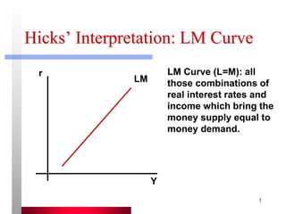
  • 1. 1 Hicks’ Interpretation: LM Curve Y r LM LM Curve (L=M): all those combinations of real interest rates and income which bring the money supply equal to money demand.
  • 2. 2 IS Curve Y r IS Slopes downward because r I Y
  • 3. The IS curve: equilibrium in the goods market  The goods market is in equilibrium when savings is equal to investment.  The IS curve shows the real interest rate for which the goods market is in equilibrium.  The IS curve is so called because at all points on it savings is equal to investment  The IS curve slopes downward because if output (income) increases, savings also increases reducing the interest rate and vice versa.  For constant output, any change in the economy that changes national savings relative to investment will change the interest rate that clears the market and shift the IS curve.  We plot IS curve only by changing savings curve (NOT investment curve), because savings determine the level of investment. 3
  • 4. The IS and the LM Relations Together Equilibrium in the goods market (IS). Equilibrium in financial markets (LM). When the IS curve intersects the LM curve, both goods and financial markets are in equilibrium. IS relation: Y     C Y T I Y i G ( ) ( , ) LM relation: M P  YL i ( ) The IS-LM Model
  • 5. Shifts of the LM Curve An increase in money... Shifts of the LM Curve
  • 6. Fiscal Policy, the Interest Rate and the IS Curve  Fiscal contraction: a fiscal policy that reduces the budget deficit. – Reducing G or increasing T  Fiscal expansion: increasing the budget deficit. – Increasing G or decreasing T  Taxes (T) and government expenditures (G) affect the IS curve, not the LM curve.
  • 7. Fiscal Policy, the Interest Rate and the IS Curve The Effects of an Increase in Taxes
  • 8. Monetary Policy, the Interest Rate, and the LM Curve  Monetary contraction (tightening) refers to a decrease in the money supply.  An increase in the money supply is called monetary expansion.  Monetary policy affects only the LM curve, not the IS curve.
  • 9. Monetary Policy, the Interest Rate, and the LM Curve The Effects of a Monetary Expansion
  • 10. Factors that shift IS curve An increase in Shifts the IS curve Reason Expected future output Up and to the right Consumption rises, savings falls, interest rate rises Wealth Up and to the right Government purchases Up and to the right Expected future MPK Up and to the right Investment increases, interest rate rises Tax No change (Ricardian Equivalence) If the consumers think that in future they will get an equivalent amount of tax-cut Down and to the left If the consumers reduce consumption because of the tax 10
  • 11. Factors that shift the LM curve An increase in Shifts the LM curve Reason M Down and to the right Reduces r as M/P increases P Up and to the left Increases r as M/P falls Down and to the right Reduces r as demand for money falls Wealth Up and to the left Demand for money increases and r increases Payment technology Down and to the right Demand for money falls and r falls 11
  • 12. Using a Policy Mix The Effects of Fiscal and Monetary Policy. Shift of IS Shift of LM Movement of Output Movement in Interest Rate Increase in taxes left none down down Decrease in taxes right none up up Increase in spending right none up up Decrease in spending left none down down Increase in money none down up down Decrease in money none up down up
  • 13. General equilibrium in the IS-LM framework: Classical vs. Keynesian debate  We have seen that an increase in the money supply will reduce the interest rate and shift the LM curve to the right to intersect the IS curve in a new point, where a temporary equilibrium only in the goods and asset market will be established.  The labor market will not be in this equilibrium and consequently firms will push the price up to return to the general equilibrium state.  The question is how fast this adjustment process takes place?  According to the Classical view the adjustment process takes place very quickly.  On the other hand, the Keynesian view proposes that the adjustment process may take long time and as a result the state out of general equilibrium may persist for a long time.  About the monetary neutrality, both agrees. The difference in their view is that- the Classical economists thinks money is always neutral and the Keynesians think that money is neutral but takes a considerable time to be neutral. 13
  • 14. 11-14 Use the IS-LM model to show how monetary and fiscal policy work – Fiscal policy has its initial impact in the goods market – Monetary policy has its initial impact mainly in the assets markets Because the goods and assets markets are interconnected, both fiscal and monetary policies have effects on both the level of output and interest rates Expansionary/contractionary monetary policy moves the LM curve to the right/left Expansionary/contractionary fiscal policy
  • 15. 11-15 Monetary Policy  The Central Bank is responsible for monetary policy  Conducted mainly through open market operations: – Buying/selling government bonds  CB buys bonds in exchange for money  stock of money goes up  CB sells bonds in exchange for money paid by purchasers of the [Insert Figure 11-3 here]
  • 16. 11-16 Monetary Policy  Consider monetary expansion  Increase in money supply creates an excess supply of money  LM curve shifts out to LM’  Public adjusts by buying other assets  Asset prices increase, and yields decrease  move to point E1  Money market clears, with lower interest rate  Decline in interest rate results in excess demand for goods: goods market out of equilibrium at E1 [Insert Figure 11-3 here, again]
  • 17. 11-17 Monetary Policy  Note the slope of the LM curve is important  Relatively flat LM curve: the shift in LM curve results in small change in interest rate and small change in output  Relatively steep LM curve: large effects [Insert Figure 11-3 here, again]
  • 18. 11-18 Transition Mechanism  Two steps in the transmission mechanism (the process by which changes in monetary policy affect AD): 1. An increase in real balances generates a portfolio disequilibrium • At the prevailing interest rate and level of income, people are holding more money than they want • Portfolio holders attempt to reduce their money holdings by buying other assets  asset prices and yields change  The change in money supply drives down interest rates
  • 19. 11-19 The Liquidity Trap  Two extreme cases arise when discussing the effects of monetary policy on the economy  the first is the liquidity trap – Liquidity trap = a situation in which the public is prepared, at a given interest rate, to hold whatever amount of money is supplied – Implies the LM curve is horizontal  changes in the quantity of money do not shift it • Monetary policy has no impact on either the interest rate or the level of income  monetary policy is powerless • Possibility of a liquidity trap at low interest rates is a notion that grew out of the theories of English economist John Maynard Keynes
  • 21. 11-21 Banks’ Reluctance to Lend  Two extreme cases arise when discussing the effects of monetary policy on the economy  the second is the reluctance of banks to lend – Despite lower interest rates and increased demand for investment, banks may be unwilling to make the loans necessary for the investment purchases – This leads to a break down in the transmission mechanism – If banks made prior bad loans that are not repaid, they may become reluctant to make more, despite demand  they prefer instead to lend to the government (safer)
  • 22. 11-22 The Classical Case  The opposite of horizontal LM curve (i.e. monetary policy cannot affect income) is vertical LM curve – If LM is vertical  demand for money unresponsive to the interest rate – The equation for the LM curve is (1) • If h is zero  there is a unique level of income corresponding to a given real money supply  VERTICAL LM CURVE  Vertical LM curve corresponds to the classical case – Rewrite equation (1), with h = 0: (2) • Implies that nominal GDP depends only on the quantity of money  quantity theory of money hi kY P M   ) ( Y P k M  
  • 23. 11-23 The Classical Case  When the LM curve is vertical 1. A given change in the quantity of money has a maximal effect on the level of income 2. Shifts in the IS curve do not affect the level of income  Only monetary policy affects income, fiscal policy is ineffective – Requires that the demand for money be irresponsive to i  important issue in determining the effectiveness of alternative policies – Evidence suggests that demand for money does depend on the interest rate
  • 24. 11-24 Fiscal Policy and Crowding Out  If the economy is initially in equilibrium at E, if government expenditures increases, equilibrium moves to E”  The goods market is in equilibrium at E”, but the money market is not  Y has increased  demand for money also increases  interest rate increases  Firms’ planned investment spending declines at higher interest rates and AD falls off  move up the LM curve to E’ [Insert Figure 11-4 here]
  • 25. 11-25 Fiscal Policy and Crowding Out  Increased government spending increases income and the interest rate  Higher interest rates and their impact on AD dampen the expansionary effect of increased G  Income increases to Y’0 instead of Y” [Insert Figure 11-4 here] Increase in government expenditures crowds out investment spending.
  • 26. 11-26 Fiscal Policy and Crowding Out  Note: slopes of IS/LM curves important  Flat LM curve:  large effect on output, small change in interest rate  Flat IS curve:  little effect on output or interest rate  The larger the multiplier, G, the further the IS curve shifts  NB: if economy at full employment, higher G raises P  real money supply falls  interest rate goes up  I falls [Insert Figure 11-4 here]
  • 27. 11-27 The Composition of Output and the Policy Mix  Table 11-2 summarizes our analysis of the effects of expansionary monetary and fiscal policy on output and the interest rate (assuming not in a liquidity trap or in the classical case)  Monetary policy operates by stimulating interest-responsive components of AD  Fiscal policy operates through G and t  impact depends upon what goods the government buys and what taxes and transfers it changes – Increase in G  increases C along with G; reduction in income taxes increases C  Accommodating monetary policy: fiscal expansion accompanied by monetary expansion: both curves shift, output increases, interest rate stays the same [Insert Table 11-2 here]
  • 28. B. Friedman’s Model C C c Y T c I i i r i Y C I G M m m Y m r m m M M M d d s                   0 1 1 0 1 1 0 1 2 2 1 0 1 0 0 ( ), , , and derives:   r m c m c i m c T c M m G m c i m            0 1 1 0 0 1 1 1 1 2 1 1 1 1 1 1 ( ) ( ) ( ) ( )
  • 29. Result Friedman finds via the total derivative that: dr dG m m c i m      1 2 1 1 1 1 0 ( ) This is positive, but how “important?” Short-run Value Long-run Value Goldfeld (M1) 0.930 0.657 Friedman (M2) 0.849 0.448 Hamburger (M3) 0.876 0.796 These are dY/dG after crowding!
  • 30. Variant: Balanced budget multiplier • The government above was free to set G and T however it wished. What if the government had to control the budget deficit, so that G = T at all times? • If we put the G = T requirement into the IS equation, we get the balanced budget multiplier: • IS Equation: Y = C(Y – T) + I + G, where C = c0 + c1 (Y – T) • Re-arranging we have: • Replace G=T, balanced budget • So our new multiplier is 1. G ) I c ( ) c 1 ( 1 Y ) G I G c c ( ) c 1 ( 1 Y 0 1 1 0 1          ) G I T c c ( ) 1 ( 1 Y 1 0 1      c
  • 31. Balanced budget multiplier • Intuition: Why is the balanced budget multiplier less than the multiplier without balancing the budget? • Answer: In the balanced budget case, the government has to raise T by $1 when it raises G by $1. Raising T will lower output but by less than G raises output. The net result is a higher level of output, but less than if the government did not have to simultaneously raise taxes.
  • 32. Portfolio Crowding Focuses on portfolio effects associated with financing debt. First, he adds wealth effects to “IS”: Y y y G y T y r y W y y y          0 1 1 2 3 3 2 1 1 0 1 ( ) , , Here W is the total real wealth in the private sector. • Assume that the balanced budget multiplier = 1. W = M + B + K Note: This implies that any asset demand is a linear combination of the other two. [There are only two independent asset demands.]
  • 33. Portfolio Crowding (2) • Assume that the initial equilibrium of IS and LM is with a balanced budget (G=T) and taxes remain unchanged. Taking differentials: dW = dM + dB Note: The Christ-Silber arguments assume that government bonds represent net wealth. • Assume fixed prices, and fixed capital stock.
  • 34. Portfolio Crowding (3) The interest rate variable r in the extended IS curve reflects expected return; it is the expected yield on real capital. So now we have two r’s, rK and rB. The extended model is now: Y y y G y T y r y M K B M m m r m r m Y m M K B B b m b r b r b Y b M K B K B K B K                        0 1 1 2 3 0 2 3 4 5 0 2 3 3 4 5 1 ( ) ( ) ( ) ( ) ( )
  • 35. Portfolio Crowding (4) dY dG y y y c     1 3 1 1 1 1 , . note that This implies that the goods market reinforces the usual 1/(1-c) multiplier effect. Given m4 > 0, increases in Y imply increases in the transactions demand for money. If the money supply is fixed, then either rB or rK, or both, must rise. (Note: m2,m3 < 0.) Friedman solves the extended model:
  • 36. Portfolio Crowding (5) RESULT: As long as assets are all gross substi- tutes, transactions crowding is out. But what about Portfolio Crowding? As money demand rises, M + K + B increases. (Recall m5 > 0.) Therefore the wealth effect reinforces the transactions effect, further increasing money demand. But does rB rise, rK rise, or both?
  • 37. Portfolio Crowding (6) Assume that 0 < b5 < 1. This amounts to saying that people don’t want to hold all of their wealth in bonds. If the bond supply changes in the absence of yield changes, either rB rises or rK falls. BUT, the effect of interest rates on the goods market depends on rK. Since we cannot know whether this rate has changed, we cannot know if crowding is “out” or “in”.
  • 38. Portfolio Crowding (6) More specifically, we can solve for the partial derivative:     r G m b m m b m m m m b m b K       2 5 2 5 3 5 2 3 2 3 3 3 1 This implies that if all three assets are substitutes (m3 , m2 , b3 < 0), then the denominator is positive, and      r G m b K  2 3 ,
  • 39. Portfolio Crowding (7) RESULT: Whether the crowding is “in” or “out” depends on whether bonds are closer portfolio substitutes for money or for capital. If bonds are closer to capital, then LM shifts leftward and crowding is “out”. If bonds are closer to money, then LM shifts rightward, reinforcing fiscal policy, and crowding is “in”.
  • 40. Deficits and Interest Rates: Empirical Evidence (1)  Paul Evans. “Do Large Deficits Produce High Interest Rates?” AER 1985.  RESULT: No Crowding  Method & Assumptions: – G, Deficits, Money Supply: Exogenous – Data 1858-1984, 2SLS  Problems: – 1858-69, capital inflows may have financed deficit – Post WWII - 1979, Fed pegged interest rates – prior to 1980s, deficits were typically small – the analysis denies the endogeneity of G, deficits, Ms
  • 41. Deficits and Interest Rates: Empirical Evidence (2)  Martin Feldstein & Otto Eckstein. “The Fundamental Determinants of the Interest Rate,” REStat 1970.  RESULT: Minimal Crowding Out.  10% increase in federal debt increased the interest rate on AAA bonds by 0.28%: 1954Q1 - 1969Q2.  Problems – Period of analysis is during the Fed interest rate pegging period, and with fixed exchange rates – Data set is not very rich, and the result (as faithfully reported by the authors) is not very strong at all.
  • 42. Deficits and Interest Rates: Empirical Evidence (3)  Girola (1984) Updates Feldstein & Epstein interest rate equation. – RESULT: No Crowding(?) – Debt has a positive, but significant effect on the interest rate, but the Durbin-Watson statistic is very low -- this implies autocorrelation in the residuals – After correction for autocorrelation, the coefficient estimate becomes negative and insignificant  Plosser (1982, 1987) – RESULT: No Crowding – Changes in privately held gov’t debt have no effect on yields of government securities
  • 43. Deficits and Interest Rates: Empirical Evidence (4)  Hoelscher (1983) – RESULT: No Crowding – 3-month T-Bill vs. deficit, unemployment, expected inflation, and the monetary base – Positive but insignificant coefficient  Barth, Iden, Russek (1984-85) Replicate Hoelscher – Decomposed the deficit into structural and cyclical components – Structural deficit has positive and significant coefficient – RESULT: Crowding Out
  • 44. Deficits and Interest Rates: Empirical Evidence (5)  Carlson (1983) – RESULT: Crowding out – Aaa corporate bond rate vs. privately-held federal debt, expected inflation, GNP, and monetary base – 1953:2 - 1983:2 – Positive and significant coefficient for debt variable, but first order serial correlation  Barth, Iden, Russek (1984-85) Replicate Carlson – Cannot repeat the Carlson result! – Positive coefficient, not significant! – RESULT: No Crowding
  • 45. Deficits and Interest Rates: Empirical Evidence (6)  Barth, Iden, Russek (1984-1985) – RESULT: Crowding Out – Positive significant relationship between the structural deficit and the interest rate  Placone, Ulbrich, Wallace (JPKE) – RESULT: Depends entirely on debt management practices. – Just as easy to get the opposite result as Barth, et al.  de Leeuw and Holloway – RESULT: Crowding Out
  • 46. Deficits and Interest Rates: Empirical Evidence (7)  CBO (1984) – Surveyed 24 studies of interest-rate/deficit relationship – Studies differed widely in terms of • time period • data frequency • statistical method • interest rate variable • deficit or debt variable – Result: • Debt is more significant than the Deficits, • Neither was significant or consistently positive