Inverse CW
•Download as DOCX, PDF•
0 likes•162 views
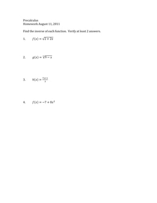
This precalculus homework document contains 4 problems asking to find the inverse of given functions and verify at least 2 answers for each inverse function. The functions given are: 1) fx=2+2x2, 2) gx=39-x, 3) hx=7x+13, and 4) fx=-7+8x2.
Report
Share
Report
Share
Recommended
boolean algebra
George Boole invented Boolean algebra in 1854 to represent logical operations using algebra. Boolean algebra uses two values, TRUE and FALSE, and defines operators like AND, OR, and NOT. It became useful for digital circuit design when Claude Shannon applied it to telephone switching circuits. Boolean algebra is defined by elements, operators, and axioms like closure, commutativity, identity, and inverse elements. The theorems of Boolean algebra can be proven using truth tables that list all possible combinations of input variables.
A1 Test 2 study guide
1. The document provides a study guide for an Algebra 1 Test 2 with questions about: graphing and writing inequalities on number lines, solving linear inequalities and compound inequalities, graphing linear inequalities on the xy-plane, and solving absolute value equations and inequalities.
2. Questions involve skills like graphing inequalities, writing inequalities from graphs, solving one-step and two-step inequalities, and solving absolute value equations and inequalities.
3. The study guide covers key Algebra 1 concepts to help prepare for Test 2.
PC Test 2 study guide 2011
1. The document is a study guide for a precalculus test that covers topics involving vectors, complex numbers, and their representations and operations.
2. It lists 15 problems involving finding magnitudes and direction of vectors, vector components, dot and cross products, complex numbers in rectangular and polar form, and converting between polar and rectangular coordinates.
3. The problems cover basic vector and complex number calculations, representations, properties and conversions.
A1 Test 3 study guide with answers
1. The solution to a system of equations is a point, while the solution to a system of inequalities is a shaded region on a graph.
2. Parallel lines have the same slope and never intersect, so they have no solution. Coinciding lines are the same single line, so they have infinitely many solutions.
3. The document provides examples of solving systems of equations and inequalities through graphing, substitution, and elimination. The solutions are given as points or descriptions of regions.
A1 12 scatter plots
Scatter plots use a series of points to represent a relationship between two variables, with the x-axis representing one variable and the y-axis representing the other. A scatter plot should include a title, labeled x-axis, and labeled y-axis. Correlation can be positive if points increase from left to right, negative if points decrease from left to right, or no correlation if points have no trend. A line of best fit shows the overall trend of the data by having the same number of points above and below the line.
A2 Test 3 with answers 2011
This study guide covers polynomials, including classifying polynomials by degree and terms, adding and subtracting polynomials, multiplying polynomials, dividing polynomials using long division and synthetic division, factoring quadratics, solving quadratics, and graphing quadratics by finding the vertex, axis of symmetry, and x-intercepts. Key concepts are polynomials having only positive integer exponents, the degree being the highest exponent, and the leading coefficient being the coefficient of the term with the highest exponent.
A1 11 functions
The document discusses functions, their domains and ranges, function notation, evaluating functions, and sequences. It provides examples of arithmetic and geometric sequences and how they can be defined using equations. It also discusses determining whether numbers are in the domain of a function and finding the domain and range of functions given their equations or graphs.
5.1graphquadratics
This document discusses quadratic functions and their graphs. It defines a quadratic function as having the form y = ax2 + bx + c. The graph of a quadratic function is a parabola, which has a vertex (lowest or highest point) and an axis of symmetry (vertical line through the vertex). It provides examples of graphing different quadratic functions using a graphing calculator and by hand, including how to find and plot the vertex and axis of symmetry.
A1 11 functions
This document covers functions, including evaluating functions at given inputs, domains and ranges of functions, and sequences. It defines arithmetic and geometric sequences, providing examples of writing equations for each type of sequence and generating additional terms. Students are asked to evaluate functions, write equations for sequences, and find subsequent terms of given arithmetic and geometric sequences.
A2 Test 2 study guide with answers (revised)
The document is an algebra 2 study guide that provides practice problems for graphing and solving various types of inequalities and systems of equations, including:
1) Graphing linear and compound inequalities on number lines and coordinate planes
2) Solving absolute value equations and inequalities
3) Solving systems of linear equations through graphing, substitution, and elimination
The study guide contains over 50 problems to help students prepare for an algebra 2 test.
A2 Test 2 study guide with answers
This document provides a study guide with answers for an Algebra 2 Test 2. It includes instructions to graph and solve various types of inequalities, systems of equations and absolute value equations, including linear and compound inequalities, systems of linear equations solved by graphing, substitution and elimination, and absolute value equations and inequalities.
A1 Test 2 study guide with answers 2011
The document is an algebra 1 test study guide containing 30 problems involving graphing and solving various types of inequalities, including linear, compound, absolute value, and graphing solutions on number lines. Key topics covered include writing inequalities from graphs, solving single-variable and compound inequalities, graphing linear inequalities on a coordinate plane, and solving absolute value equations and inequalities.
PCExam 1 practice with answers
1. This practice exam covers topics like complex numbers, functions, limits, and graphing.
2. It asks students to choose problems involving adding, multiplying, composing, and finding inverses of various functions like f(x)=9x^2+1 and g(x)=x-1.
3. Students also must graph and classify functions, evaluate limits, and perform operations on complex numbers, plotting them on a plane. The exam covers concepts in precalculus.
PCExam 1 study guide answers
1. The document provides examples and definitions for various mathematical concepts including natural numbers, integers, rational numbers, real numbers, imaginary numbers, and complex numbers.
2. It also includes problems involving composition of functions, finding inverses of functions, operations on complex numbers, graphing and classifying functions, and evaluating limits.
3. Examples cover topics like composition and inverses of functions, operations on complex numbers, classifying functions as linear, quadratic, constant, etc. and their domains and ranges, and evaluating limits including ones that are undefined.
PC Exam 1 study guide
This study guide covers topics in precalculus including:
1) Examples of natural numbers, integers, rational numbers, and real numbers.
2) Composition of functions including finding f(g(x)) and g(f(x)) for given functions f(x) and g(x).
3) Finding inverses of functions and verifying inverses by composition.
4) Operations on complex numbers including plotting, finding modulus, distance, midpoint, addition, subtraction, multiplication, and division.
5) Graphing functions, classifying function types, and stating domains and ranges.
6) Finding limits of functions as x approaches values.
PC 1 continuity notes
A continuous function is defined as one that is defined at a point c, where the limit exists and the function approaches the same y-value from both sides of point c. A function may be discontinuous due to an infinite jump, a jump, or a point discontinuity. Rational functions are defined as the quotient of two polynomial functions. They have asymptotes which occur where the denominator is zero, creating either a vertical or horizontal asymptote in the graph. The end behavior of functions can be determined by considering whether they are increasing or decreasing over different intervals.
PC 1 continuity
This document discusses continuity and discontinuities in functions, defining continuous functions as smooth curves where the domain includes all real numbers. It presents tests for continuity, requiring a function to be defined at a point, have an existing function value, and approach the same y-value from both sides. Critical points and extrema are defined as maximums where a function changes from increasing to decreasing, and minimums where it changes from decreasing to increasing. Rational functions are described as the quotient of two polynomial functions, with limited domains and possible vertical asymptotes.
A1 3 linear fxns
The document discusses the slope-intercept form of a linear equation, y=mx+b. It explains that x represents the input, y represents the output, m is the slope of the line, and b is the y-intercept. It provides instructions for graphing a linear equation in slope-intercept form, which is to first plot the y-intercept and then use the slope to rise and run to the next point, connecting the points with a line.
A1 3 linear fxns notes
The document discusses slope and linear equations. It defines slope as rise over run and provides examples of calculating slope from graphs and ordered pairs. It also defines the standard form of a linear equation as y=mx+b, where m is the slope and b is the y-intercept. The document explains how to graph lines from their equations in standard form by plotting the y-intercept and using the slope to rise and run to the next point.
A1 2 linear fxns
This document discusses the slope-intercept form of a linear equation, y=mx+b. It explains that x represents the input, y represents the output, m is the slope of the line, and b is the y-intercept. It provides instructions for graphing a linear equation in slope-intercept form, which is to first plot the y-intercept, then use the slope to rise and run to the next point and connect them with a line.
A1 2 linear fxns notes
This document discusses intercepts and slope of lines in algebra 1. It defines x-intercepts as where the line crosses the x-axis and y-intercepts as where it crosses the y-axis. It provides the equations for finding each, and includes two examples of finding intercepts and graphing lines. It also defines slope as rise over run and asks what the slope is of a given graph, with homework assigned on slope of lines and graphing lines intuitively.
A2 2 linear fxns notes
This document provides instructions and examples for finding the slope and y-intercept of a line from its equation, ordered pairs, or graph and using them to graph the line. It explains that slope is defined as rise over run and is used along with the y-intercept to graph lines by standard form, plotting the y-intercept and using slope to find successive points. Exercises are provided to have students practice finding slope, y-intercept, and graphing lines from different representations.
A2 3 linear fxns
This document provides examples and instructions for writing linear equations in slope-intercept form using different information about a line. It explains that to write the equation you need the slope and y-intercept, and gives examples of finding these values when given the slope and a point, or when given two points to calculate the slope. The document emphasizes that a point on the line satisfies the equation and shows how to use the slope and a point to determine the y-intercept and write the final equation.
A2 3 linear fxns notes
The document provides examples for finding the equation of a line given certain information. Example 1 asks to find the slope of a line passing through two points. Example 2 gives the slope and y-intercept and asks for the equation in slope-intercept form. Example 3 gives the slope and a point and asks for the equation. Example 4 asks for the equation of a line passing through two given points.
A1 1 linear fxns
Linear functions create a straight line on a graph where each point (x, y) that satisfies the linear equation lies. The document outlines how to graph linear functions by creating a table of x-values to plug into the linear equation to find the corresponding y-values, plotting these points and connecting them with a straight line.
A1 1 linear fxns notes
A linear function creates a straight line graph. A solution to a linear equation is a point on the line. The graph of a linear function is the set of all points (x, y) that satisfy the linear equation, with all these points forming a straight line. One way to graph a linear function is to choose sample x-values, calculate the corresponding y-values using the linear equation, plot these points, and connect them with a straight line.
A2 1 linear fxns notes
1. A linear function is a pairing of input and output values that can be represented graphically by a set of points that form a straight line.
2. A relation is a function when each input value has exactly one output value.
3. The graph of a linear equation is the set of all ordered pairs (x, y) that satisfy the linear equation, which together form a straight line.
A2 1 linear fxns
This document discusses linear functions and how to graph them. It defines relations and functions, noting that a function has each input mapped to only one output. It states that a linear function forms a straight line on a graph. Methods for graphing linear functions include creating a table of x- and y-values by plugging inputs into the linear equation and plotting the points, or finding the x- and y-intercepts where the line crosses the axes.
More Related Content
More from vhiggins1
A1 11 functions
This document covers functions, including evaluating functions at given inputs, domains and ranges of functions, and sequences. It defines arithmetic and geometric sequences, providing examples of writing equations for each type of sequence and generating additional terms. Students are asked to evaluate functions, write equations for sequences, and find subsequent terms of given arithmetic and geometric sequences.
A2 Test 2 study guide with answers (revised)
The document is an algebra 2 study guide that provides practice problems for graphing and solving various types of inequalities and systems of equations, including:
1) Graphing linear and compound inequalities on number lines and coordinate planes
2) Solving absolute value equations and inequalities
3) Solving systems of linear equations through graphing, substitution, and elimination
The study guide contains over 50 problems to help students prepare for an algebra 2 test.
A2 Test 2 study guide with answers
This document provides a study guide with answers for an Algebra 2 Test 2. It includes instructions to graph and solve various types of inequalities, systems of equations and absolute value equations, including linear and compound inequalities, systems of linear equations solved by graphing, substitution and elimination, and absolute value equations and inequalities.
A1 Test 2 study guide with answers 2011
The document is an algebra 1 test study guide containing 30 problems involving graphing and solving various types of inequalities, including linear, compound, absolute value, and graphing solutions on number lines. Key topics covered include writing inequalities from graphs, solving single-variable and compound inequalities, graphing linear inequalities on a coordinate plane, and solving absolute value equations and inequalities.
PCExam 1 practice with answers
1. This practice exam covers topics like complex numbers, functions, limits, and graphing.
2. It asks students to choose problems involving adding, multiplying, composing, and finding inverses of various functions like f(x)=9x^2+1 and g(x)=x-1.
3. Students also must graph and classify functions, evaluate limits, and perform operations on complex numbers, plotting them on a plane. The exam covers concepts in precalculus.
PCExam 1 study guide answers
1. The document provides examples and definitions for various mathematical concepts including natural numbers, integers, rational numbers, real numbers, imaginary numbers, and complex numbers.
2. It also includes problems involving composition of functions, finding inverses of functions, operations on complex numbers, graphing and classifying functions, and evaluating limits.
3. Examples cover topics like composition and inverses of functions, operations on complex numbers, classifying functions as linear, quadratic, constant, etc. and their domains and ranges, and evaluating limits including ones that are undefined.
PC Exam 1 study guide
This study guide covers topics in precalculus including:
1) Examples of natural numbers, integers, rational numbers, and real numbers.
2) Composition of functions including finding f(g(x)) and g(f(x)) for given functions f(x) and g(x).
3) Finding inverses of functions and verifying inverses by composition.
4) Operations on complex numbers including plotting, finding modulus, distance, midpoint, addition, subtraction, multiplication, and division.
5) Graphing functions, classifying function types, and stating domains and ranges.
6) Finding limits of functions as x approaches values.
PC 1 continuity notes
A continuous function is defined as one that is defined at a point c, where the limit exists and the function approaches the same y-value from both sides of point c. A function may be discontinuous due to an infinite jump, a jump, or a point discontinuity. Rational functions are defined as the quotient of two polynomial functions. They have asymptotes which occur where the denominator is zero, creating either a vertical or horizontal asymptote in the graph. The end behavior of functions can be determined by considering whether they are increasing or decreasing over different intervals.
PC 1 continuity
This document discusses continuity and discontinuities in functions, defining continuous functions as smooth curves where the domain includes all real numbers. It presents tests for continuity, requiring a function to be defined at a point, have an existing function value, and approach the same y-value from both sides. Critical points and extrema are defined as maximums where a function changes from increasing to decreasing, and minimums where it changes from decreasing to increasing. Rational functions are described as the quotient of two polynomial functions, with limited domains and possible vertical asymptotes.
A1 3 linear fxns
The document discusses the slope-intercept form of a linear equation, y=mx+b. It explains that x represents the input, y represents the output, m is the slope of the line, and b is the y-intercept. It provides instructions for graphing a linear equation in slope-intercept form, which is to first plot the y-intercept and then use the slope to rise and run to the next point, connecting the points with a line.
A1 3 linear fxns notes
The document discusses slope and linear equations. It defines slope as rise over run and provides examples of calculating slope from graphs and ordered pairs. It also defines the standard form of a linear equation as y=mx+b, where m is the slope and b is the y-intercept. The document explains how to graph lines from their equations in standard form by plotting the y-intercept and using the slope to rise and run to the next point.
A1 2 linear fxns
This document discusses the slope-intercept form of a linear equation, y=mx+b. It explains that x represents the input, y represents the output, m is the slope of the line, and b is the y-intercept. It provides instructions for graphing a linear equation in slope-intercept form, which is to first plot the y-intercept, then use the slope to rise and run to the next point and connect them with a line.
A1 2 linear fxns notes
This document discusses intercepts and slope of lines in algebra 1. It defines x-intercepts as where the line crosses the x-axis and y-intercepts as where it crosses the y-axis. It provides the equations for finding each, and includes two examples of finding intercepts and graphing lines. It also defines slope as rise over run and asks what the slope is of a given graph, with homework assigned on slope of lines and graphing lines intuitively.
A2 2 linear fxns notes
This document provides instructions and examples for finding the slope and y-intercept of a line from its equation, ordered pairs, or graph and using them to graph the line. It explains that slope is defined as rise over run and is used along with the y-intercept to graph lines by standard form, plotting the y-intercept and using slope to find successive points. Exercises are provided to have students practice finding slope, y-intercept, and graphing lines from different representations.
A2 3 linear fxns
This document provides examples and instructions for writing linear equations in slope-intercept form using different information about a line. It explains that to write the equation you need the slope and y-intercept, and gives examples of finding these values when given the slope and a point, or when given two points to calculate the slope. The document emphasizes that a point on the line satisfies the equation and shows how to use the slope and a point to determine the y-intercept and write the final equation.
A2 3 linear fxns notes
The document provides examples for finding the equation of a line given certain information. Example 1 asks to find the slope of a line passing through two points. Example 2 gives the slope and y-intercept and asks for the equation in slope-intercept form. Example 3 gives the slope and a point and asks for the equation. Example 4 asks for the equation of a line passing through two given points.
A1 1 linear fxns
Linear functions create a straight line on a graph where each point (x, y) that satisfies the linear equation lies. The document outlines how to graph linear functions by creating a table of x-values to plug into the linear equation to find the corresponding y-values, plotting these points and connecting them with a straight line.
A1 1 linear fxns notes
A linear function creates a straight line graph. A solution to a linear equation is a point on the line. The graph of a linear function is the set of all points (x, y) that satisfy the linear equation, with all these points forming a straight line. One way to graph a linear function is to choose sample x-values, calculate the corresponding y-values using the linear equation, plot these points, and connect them with a straight line.
A2 1 linear fxns notes
1. A linear function is a pairing of input and output values that can be represented graphically by a set of points that form a straight line.
2. A relation is a function when each input value has exactly one output value.
3. The graph of a linear equation is the set of all ordered pairs (x, y) that satisfy the linear equation, which together form a straight line.
A2 1 linear fxns
This document discusses linear functions and how to graph them. It defines relations and functions, noting that a function has each input mapped to only one output. It states that a linear function forms a straight line on a graph. Methods for graphing linear functions include creating a table of x- and y-values by plugging inputs into the linear equation and plotting the points, or finding the x- and y-intercepts where the line crosses the axes.
More from vhiggins1 (20)
Inverse CW
- 1. Precalculus<br />Homework August 11, 2011<br />Find the inverse of each function. Verify at least 2 answers.<br />1.fx=2+2x<br />2.gx=39-x<br />3.hx=7x+13<br />4.fx=-7+8x2<br />