The document discusses various approaches to inventory decision making and management. It begins by outlining the key learning objectives which include understanding different inventory management approaches like EOQ, JIT, MRP, and DRP. It then explains the basic EOQ (Economic Order Quantity) model and how it can be applied under conditions of certainty and uncertainty. The document also discusses fixed order interval approaches and compares EOQ to other approaches like JIT. It provides examples and diagrams to illustrate inventory management concepts.

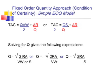
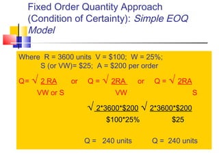
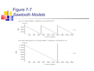
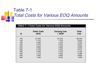
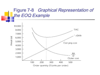
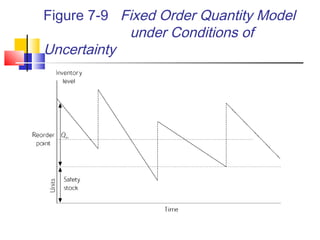
1. Chapter 7:
Inventory Decision Making

2. Learning Objectives - After reading this
chapter, you should be able to do the following:
 Understand the fundamental differences
among approaches to managing inventory.
 Appreciate the rationale and logic behind the
Economic Order Quantity (EOQ) approach to
inventory decision making, and be able to
solve some problems of a relatively
straightforward nature.
 Understand alternative approaches to
managing inventory --- JIT, MRP, and DRP.

3. Learning Objectives
 Realize how variability in demand and order
cycle length affects inventory decision
making.
 Know how inventory will vary as the number
of stocking points decreases or increases.
 Recognize the contemporary interest in and
relevance of time-based approaches to
inventory management.

4. Learning Objectives
 Make needed adjustments to the basic EOQ
approach to respond to several special types
of applications.

5. Fundamental Approaches to
Managing Inventory
 Basic issues are simple…how much to order
and when to order.
 Additional issues are…where to store inventory
and what items to order.
 Traditionally, conflicts were usually present…as
customer service levels increased, investment
in inventory also increased.
 Recent emphasis is on increasing customer
service and reducing inventory investment.

6. Fundamental Approaches to
Managing Inventory
 Four factors might permit this apparent
paradox, that is, the firm can achieve higher
levels of customer service without actually
increasing inventory:
 More responsive order processing
 Ability to strategically manage logistics data
 More capable and reliable transportation
 Improvements in the location of inventory

7. Figure 7-1 Relationship between
Inventory and Customer Service Level

8. Key Differences among
Approaches to Managing Inventory
 Dependent versus Independent Demand
 Dependent demand is directly related to the
demand for another product.
 Independent demand is unrelated to the
demand for another product.
 For many manufacturing processes,
demand is dependent.
 For many end-use items, demand is
independent.

9. Key Differences among
Approaches to Managing Inventory
 Of the inventory management processes in
this chapter, JIT, MRP and MRPII are
generally associated with items having
dependent demand.
 Alternatively, DRP and the EOQ models are
generally associated with items exhibiting
independent demand.

10. Key Differences among
Approaches to Managing Inventory
 Pull versus Push
 Pull approach is a “reactive” system, relying
on customer demand to “pull” product
through a logistics system. MacDonald’s is
an example.
 Push approach is a “proactive” system, and
uses inventory replenishment to anticipate
future demand. Catering businesses are
examples of push systems.

11. Key Differences among
Approaches to Managing Inventory
 Pull versus Push
 Pull systems respond quickly to sudden or
abrupt changes in demand, involve one-way
communications, and apply more to
independent demand situations.
 Push systems use an orderly and disciplined
master plan for inventory management, and
apply more to dependent demand situations.

12. On the Line:
American Cancer Society
 ACS constructed a world class automated order
fulfillment center in Atlanta.
 Order cycle time was reduced to five business
days.
 Centralized storage reduced waste and
obsolescence of educational materials.
 Centralized shipment reduced freight rates.
 The new center saved $8 million in the first year
alone.

13. Fixed Order Quantity Approach
(Condition of Certainty): Inventory Cycles
 In this example, each cycle starts
with 4,000 units:
 Demand is constant at the rate of
800 units per day.
 When inventory falls below 1,500 units, an
order is placed for an additional 4,000 units.
 After 5 days the inventory is completely used.
 Just as the 4,000th unit is sold, the next order
of 4,000 units arrives and a new cycle begins.

14. Figure 7-2 Fixed Order Quantity
Model under the Condition of Certainty

15. Fixed Order Quantity Approach
(Condition of Certainty): Simple EOQ
Model
 Simple EOQ Model Assumptions
 Continuous, constant, known and infinite rate
of demand on one item of inventory.
 A constant and known replenishment time.
 Satisfaction of all demand.
 Constant cost, independent of order quantity
or time.
 No inventory in transit costs.
 No limits on capital availability.

16. Fixed Order Quantity Approach
(Condition of Certainty): Simple EOQ
Model
 Simple EOQ Model Variables
 R = annual rate of demand
 Q = quantity ordered (lot size in units)
 A = order or setup cost
 V = value or cost of one unit in dollars
 W = carrying cost per dollar value in percent
 S = VW = annual storage cost in $/unit per year
 t = time in days
 TAC = total annual costs in dollars per year

17. Figure 7-3
Inventory Carrying Cost

18. Figure 7-4
Order or Setup Cost

19. Figure 7-5
Inventory Costs

20. Fixed Order Quantity Approach (Condition
of Certainty): Simple EOQ Model
TAC = QVW + AR or TAC = QS + AR
2 Q 2 Q
First term is the average carrying cost
Second term is order or setup costs per year

21. Figure 7-6
Sawtooth Model

22. Fixed Order Quantity Approach (Condition
of Certainty): Simple EOQ Model
TAC = QVW + AR or TAC = QS + AR
2 Q 2 Q
Solving for Q gives the following expressions:
Q= √ 2 RA or Q = √ 2RA or Q = √ 2RA
VW or S VW S

23. Fixed Order Quantity Approach
(Condition of Certainty): Simple EOQ
Model
Where R = 3600 units V = $100; W = 25%;
S (or VW)= $25; A = $200 per order
Q= √ 2 RA or Q = √ 2RA or Q = √ 2RA
VW or S VW S
√ 2*3600*$200 √ 2*3600*$200
$100*25% $25
Q = 240 units Q = 240 units

24. Figure 7-7
Sawtooth Models

25. Table 7-1
Total Costs for Various EOQ Amounts

26. Figure 7-8 Graphical Representation of
the EOQ Example

27. Fixed Order Quantity Approach
(Condition of Certainty)
 Summary and Evaluation of the Fixed
Order Quantity Approach:
 EOQ is a popular inventory model.
 EOQ doesn’t handle multiple locations as well as a
single location.
 EOQ doesn’t do well when demand is not constant.
 Minor adjustments can be made to the basic model.
 Newer techniques will ultimately take the place of EOQ.

28. Fixed Order Quantity Approach
(Condition of Uncertainty)
 Uncertainty is a more normal condition.
 Demand is often affected by exogenous
factors---weather, forgetfulness, etc.
 Lead times often vary regardless of carrier
intentions.
 Examine out Figure 7-9.
 Note the variability in lead times and
demand.

29. Figure 7-9 Fixed Order Quantity Model
under Conditions of
Uncertainty

30. Fixed Order Quantity Approach
(Condition of Uncertainty)
 Reorder Point – A Special Note
 With uncertainty of demand, the reorder
point becomes the average daily demand
during lead time plus the safety stock.
 Examine Figure 7-9 again.

31. Fixed Order Quantity Approach
(Condition of Uncertainty)
 Uncertainty of Demand Affects Simple EOQ
Model Assumptions:
 a constant and known replenishment time.
 constant cost/price, independent of order
quantity or time.
 no inventory in transit costs.
 one item and no interaction among the
inventory items.
 infinite planning horizon.
 no limit on capital availability.

32. Table 7-2 Probability Distribution
of Demand during Lead Time
Demand Probability
100 units 0.01
110 0.06
120 0.24
130 0.38
140 0.24
150 0.06
160 0.01

33. Table 7-3 Possible Units of Inventory
Short or in Excess during Lead Time with
Various Reorder Points
Actual
Demand
Reorder Points
100 110 120 130 140 150 160
100 0 10 20 30 40 50 60
110 -10 0 10 20 30 40 50
120 -20 -10 0 10 20 30 40
130 -30 -20 -10 0 10 20 30
140 -40 -30 -20 -10 0 10 20
150 -50 -40 -30 -20 -10 0 10
160 -60 -50 -40 -30 -20 -10 0

34. Table 7-3 Possible Units of Inventory
Short or in Excess during Lead Time with
Various Reorder Points
Actual
Demand
Proba-
bility
Reorder Points
100 110 120 130 140 150 160
100 0.01 0.0 0.1 0.2 0.3 0.4 0.5 0.6
110 0.06 -0.6 0 0.6 1.2 1.8 2.4 3.0
120 0.24 -4.8 -2.4 0 2.4 4.8 7.2 9.6
130 0.38 -11.4 -7.6 -3.8 0 3.8 7.6 11.4
140 0.24 -9.6 -7.2 -4.8 -2.4 0 2.4 4.8
150 0.06 -3.0 -2.4 -1.8 -1.2 -0.6 0 0.6
160 0.01 -0.6 -0.5 -0.4 -0.3 -0.2 -0.1 0

35. Table 7-4 Calculation of Lowest-Cost Reorder Point
Dmnd 100 110 120 130 140 150 160
(e) 0.0 0.1 0.8 3.9 10.8 20.1 30.0
(VW) 0 $2.50 $20 $97.50 $270 $502.50 $750
(g) 30 20.1 10.8 3.9 0.8 0.1 0.0
G=gw $300 $201 $108 $39 $8 $1 $0
GR/Q $4500 $3015 $1620 $585 $120 $15 $0
TAC $4500 $3018 $1640 $682.50 $390 $517.50 $750

36. Fixed Order Quantity Approach
(Condition of Certainty): Expanded EOQ
Model
Where R = 3600 units V = $100; W = 25%;
A = $200 per order; G = 8
Q= √ 2 R(A + G)
VW
√ 2 * 3600 * ($200 + 8)
$100 * 25%
Q = approximately 242 units

37. Fixed Order Quantity Approach
(Condition of Certainty): Expanded EOQ
Model
Where R = 3600 units V = $100; W = 25%;
A = $200 per order; G = 8; Q = 242; e = 10.8
TAC = QVW + AR + eVW + GR
2 Q Q
TAC = (242*$100*25%) + (200*3600) + (10.8*$100*25%) + (8*3600)
2 242 242
TAC = $3025 + $2975 + $270 + $119
TAC = $6389 (New value for TAC when uncertainty introduced)

38. Fixed Order Quantity Approach
(Condition of Uncertainty): Conclusions
 Following costs will rise to cover the uncertainty:
 Stockout costs.
 Inventory carrying costs of safety stock
 Results may or may not be significant.
 In text example, TAC rose $389 or
approximately 6.5%.
 The greater the dispersion of the probability
distribution, the greater the cost disparity.

39. Figure 7-10
Area under the Normal Curve

40. Table 7-5 Reorder Point Alternatives and
Stockout Possibilities

41. Fixed Order Interval Approach
 A second basic approach
 Involves ordering at fixed intervals and
varying Q depending upon the remaining
stock at the time the order is placed.
 Less monitoring than the basic model
 Examine Figure 7-11.
 Amount ordered over each five weeks in the
example varies each week.

42. Figure 7-11 Fixed Order Interval Model
(with Safety Stock)

43. Summary and Evaluation of EOQ
Approaches to Inventory Management
 Four basic inventory models:
 Fixed quantity/fixed interval
 Fixed quantity/irregular interval
 Irregular quantity/fixed interval
 Irregular quantity/irregular interval
 Where demand and lead time are known,
basic EOQ or fixed order interval model best.
 If demand or lead time varies, then safety
stock model should be used

44. Summary and Evaluation of EOQ
Approaches to Inventory Management
 Relationship to ABC analysis
 “A” items suited to a fixed quantity/irregular
interval approach.
 “C” items best suited to a irregular
quantity/fixed interval approach.
 Importance of trade-offs
 Familiarity with EOQ approaches assists the
manager in trade-offs inherent in inventory
management.

45. Summary and Evaluation of EOQ
Approaches to Inventory Management
 New concepts
 JIT, MRP, MRPII, DRP, QR, and ECR also
take into account a knowledge and
understanding of applicable logistics trade-offs.
 Number of DCs
 The issue of inventory at multiple locations in a
logistics network raises some interesting
questions concerning the number of DCs, the
SKUs at each, and their strategic positioning.

46. Additional Approaches to
Inventory Management
 Three approaches to inventory management
that have special relevance to supply chain
management:
 JIT (Just in Time)
 MRP (Materials Requirements into
Planning)
 DRP (Distribution Resource Planning)

47. Time-Based Approaches to
Replenishment Logistics: JIT
 Definition and Components of JIT Systems - designed
to manage lead times and eliminate waste.
 Kanban - refers to the informative signboards on
carts in a Toyota system of delivering parts to the
production line. Each signboard details the exact
quantities and necessary time of replenishment.
 JIT operations - Kanban cards and light warning
system communicate possible production
interruptions.
 Fundamental concepts - JIT can substantially
reduce inventory and related costs.

48. Time-Based Approaches to
Replenishment Logistics: JIT
 Definition and Components of JIT Systems -
designed to manage lead times and eliminate
waste.
 Goal is zero inventory, and zero defects.
 Similarity to the two-bin system - one bin fills
demand for part, the other is used when the
first is empty.
 Reduces lead times through requiring small
and frequent replenishment.

49. Time-Based Approaches to
Replenishment Logistics: JIT
 JIT is a widely used and effective strategy for
managing the movement of parts, materials,
semi-finished products from points of supply
to production facilities.
 Product should arrive exactly when a firm
needs it, with no tolerance for early or late
deliveries.
 JIT systems place a high priority on short,
consistent lead times.

50. JIT versus EOQ Approaches to
Inventory Management
 Six major differences:
 First, JIT attempts to eliminate excess
inventories for both buyer and seller.
 Second, JIT systems involve short
production runs with frequent changeovers.
 Third, JIT minimizes waiting lines by
delivering goods when and where needed.

51. JIT versus EOQ Approaches to
Inventory Management
 Fourth, JIT uses short, consistent lead
times to satisfy inventory needs in a timely
manner.
 Fifth, JIT relies on high-quality incoming
products and on exceptionally high-quality
inbound logistics operations.
 Sixth, JIT requires a strong, mutual
commitment between buyer and seller,
emphasizing quality and win-win outcomes
for both partners.

52. Table 7-6 EOQ versus JIT Attitudes and
Behaviors

53. Time-Based Approaches to
Replenishment Logistics: JIT
 JIT versus Traditional Inventory Management
 Reduces excess inventories
 Shorter, more frequent production runs
 Minimize waiting lines by delivering materials when
and where needed
 Short, consistent lead times through proximate
location
 Quality stressed throughout supply chain
 Win-win relationships necessary to a healthy supply
chain

54. Time-Based Approaches to
Replenishment Logistics: JIT
 Examples of JIT Successes:
 Apple Computer’s increase in IT from 10 weeks
to 2 weeks resulted in 18-month $20 million
payback on plant.
 GM increased production by 100%, but
inventories increased by only 6%.
 Norfolk Southern mini-train hauls direct from
one GM plant to another without switching
delays.
 Ryder handles all inbound logistics for Saturn.

55. Figure 7-12
The Orderly Pickup Concept

56. Time-Based Approaches to
Replenishment Logistics: MRP
 A Materials Requirements Planning (MRP)
system consists of a set of logically related
procedures, decision rules, and records
designed to translate a master production
schedule into time-phased net inventory
requirements for each component item
needed to implement this schedule.
 MRPs re-plan net requirements based on
changes in schedule, demand, etc.

57. Time-Based Approaches to
Replenishment Logistics: MRP
 Goals of an MRP:
 Ensure the availability of materials,
components, and products for
planned production.
 Maintain lowest possible inventory level.
 Plan manufacturing activities, delivery
schedules, and purchasing activities.

58. Time-Based Approaches to
Replenishment Logistics: MRP
 Key elements of an MRP:
 Master production schedule
 Bill of materials file
 Inventory status file
 MRP program
 Outputs and reports

59. Figure 7-13
An MRP System
Master Production Schedule
MRP Program
Output and Reports
Bill of Material File Inventory Status File
Customer Orders Demand Forecasts

60. Figure 7-14 Relationship of Parts to
Finished Product: MRP Egg Timer Example
1 Egg Timer
2 Ends 1 Bulb 3 Supports
1 Gram of Sand

61. Table 7-7 Inventory Status File:
MRP Egg Timer Example
Product
Gross
Req.
Inventory Net Req. Lead Time
Egg Timers 1 0 1 1
Ends 2 0 2 5
Supports 3 2 1 1
Bulbs 1 0 1 1
Sand 1 0 1 4

62. Figure 7-15 Master Schedule: MRP
Egg Timer Example

63. Time-Based Approaches to
Replenishment Logistics: MRP
 Principal advantages of MRP:
 Maintain reasonable safety stock.
 Minimize or eliminate inventories.
 Identification of process problems.
 Production schedules based on actual
demand.
 Coordination of materials ordering.
 Most suitable for batch or intermittent
production schedules.

64. Time-Based Approaches to
Replenishment Logistics: MRP
 Principal shortcomings of MRP:
 Computer intensive.
 Difficult to make changes once operating.
 Ordering and transportation costs may rise.
 Not usually as sensitive to short-term
fluctuations in demand.
 Frequently become quite complex.
 May not work exactly as intended.

65. Time-Based Approaches to
Replenishment Logistics: Distribution
Resource Planning
 MRP sets a master production schedule and
“explodes” into gross and net requirements.
 DRP starts with customer demand and works
backwards toward establishing a realistic
system-wide plan for ordering the necessary
finished products.
 Then DRP works to develop a time-phased
plan for distributing product from plants and
warehouses to the consumer.

66. Time-Based Approaches to
Replenishment Logistics: Distribution
Resource Planning
 DRP develops a projection for each SKU and
requires17
:
 Forecast of demand for each SKU.
 Current inventory level for each SKU.
 Target safety stock.
 Recommended replenishment quantity.
 Lead time for replenishment.

67. Table 7-8 DRP Table for
Chicken Noodle Soup
Columbus Distribution Center–Distribution Resource Planning
Month January February March
Week 1 2 3 4 5 6 7 8 9
CN Soup Current BOH=4314; Q=3800; SS=1956; LT=1
Forecast 974 974 974 974 989 1002 1002 1002 1061
Schedule
Receipt
0 0 3800 0 0 0 3800 0 0
BOH-End 3340 2366 5192 4218 3229 2227 5025 4023 2962
Planned
Order
0 3800 0 0 0 3800 0 0 3800

68. Figure 7-16
Combining DRP Tables

69. Inventory at Multiple Locations –
The Square Root Law (SQL)
 Used to reduce inventory at multiple locations.
 As locations increase, inventory also
increases, but not in the same ratio as the
growth in facilities.
 The square root law (SRL) states that total
safety stock can be approximated by
multiplying the total inventory by the square
root of the number of future facilities divided by
the current number of facilities.

70. Inventory at Multiple Locations –
The Square Root Law

X2= (X1) * √(n2/n1)
 Where:
 n1 = number of existing facilities
 n2 = number of future facilities
 X1 = total inventory in existing facilities
 X2 = total inventory in future facilities

71. Square Root Law Example
 Current distribution 40,000 units
 Eight facilities shrinking to two
 Using the square root law:

X2 = (40,000) * √(2/8)
 X2 = 20,000 units

72. Table 7-9 Example Impacts of Square Root
Law on Logistics Inventories
Warehouses √n Total Av Inv % Change
1 1.0000 3,885 ---
2 1.4142 5,494 141%
3 1.7321 6,729 173%
4 2.0000 7,770 200%
5 2.2361 8,687 224%
10 3.1623 12,285 316%
15 3.8730 15,047 387%
20 4.4721 17,374 447%
23 4.7958 18,632 480%
25 5.0000 19,425 500%

73. Figure 7-17 Four Directions for
Replenishment Logistics

74. Time-Based Approaches to
Replenishment Logistics: Quick
Response (QR)
 Structure of QR
 Shorter, compressed time horizons.
 Real-time information available by SKU.
 Seamless, integrated logistics networks
with rapid transportation, cross-docking
and effective store receipt and distribution
systems.

75. Time-Based Approaches to
Replenishment Logistics: Quick
Response (QR)
 Structure of QR
 Partnership relationships present among
supply chain members.
 Redesign of manufacturing processes to
reduce lot sizes, changeover times and
enhanced flexibility.
 Commitment to TQM.

76. Figure 7-18
Basic Elements of Quick Response (QR)

77. Time-Based Approaches to Replenishment
Logistics: Efficient Consumer Response
(ECR)
 Structure of ECR
 Grocery industry estimates U.S. savings at
approximately $30 billion.
 “Ultimate goal is a responsive, consumer-driven
system in which distributors and suppliers work
together as business allies to maximize consumer
satisfaction and minimize cost. Accurate
information and high-quality products flow through
a paperless system between manufacturing and
check-out counter with minimum degradation or
interruption…”

78. Figure 7-19 Efficient Consumer
Response: Broad Operating Capabilities
Tailored to Each Unique Partner

79. Chapter 7:
Summary and Review Questions
Students should review their knowledge of the chapter
by checking out the Summary and Study Questions
for Chapter 7.
This is the last slide for Chapter 7

80. Figure A7-1 Sawtooth Model Modified for
Inventory in Transit

81. Figure A7-2 EOQ Costs Considering
Volume Transportation Rate

82. Table 7A-1 Annual Savings, Annual
Cost, and Net Savings by Various
Quantities Using Incentive Rates

83. Figure A7-3 Net Savings Function for
Incentive Rate

84. End of Chapter 7 and 7A Slides
Inventory Decision Making