Download to read offline
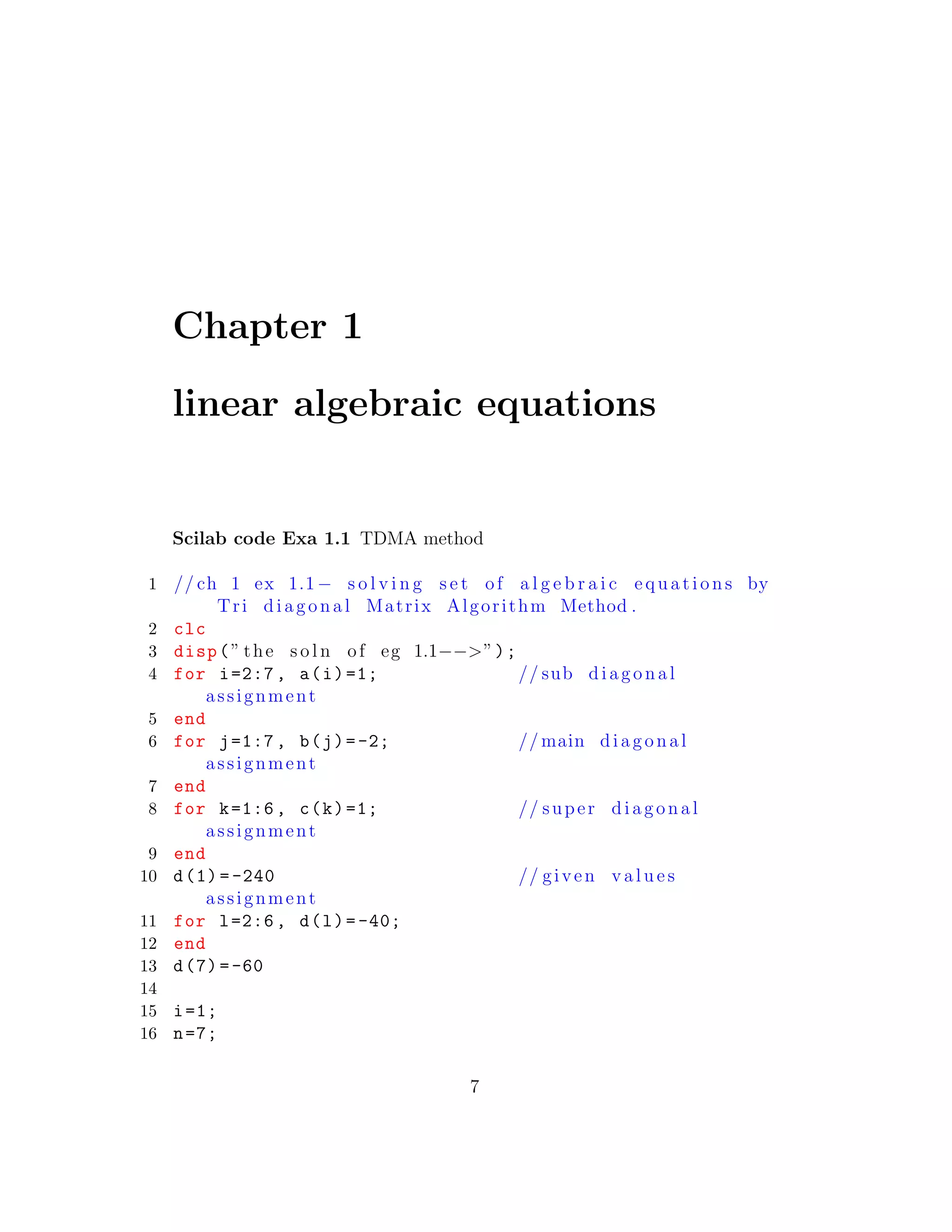
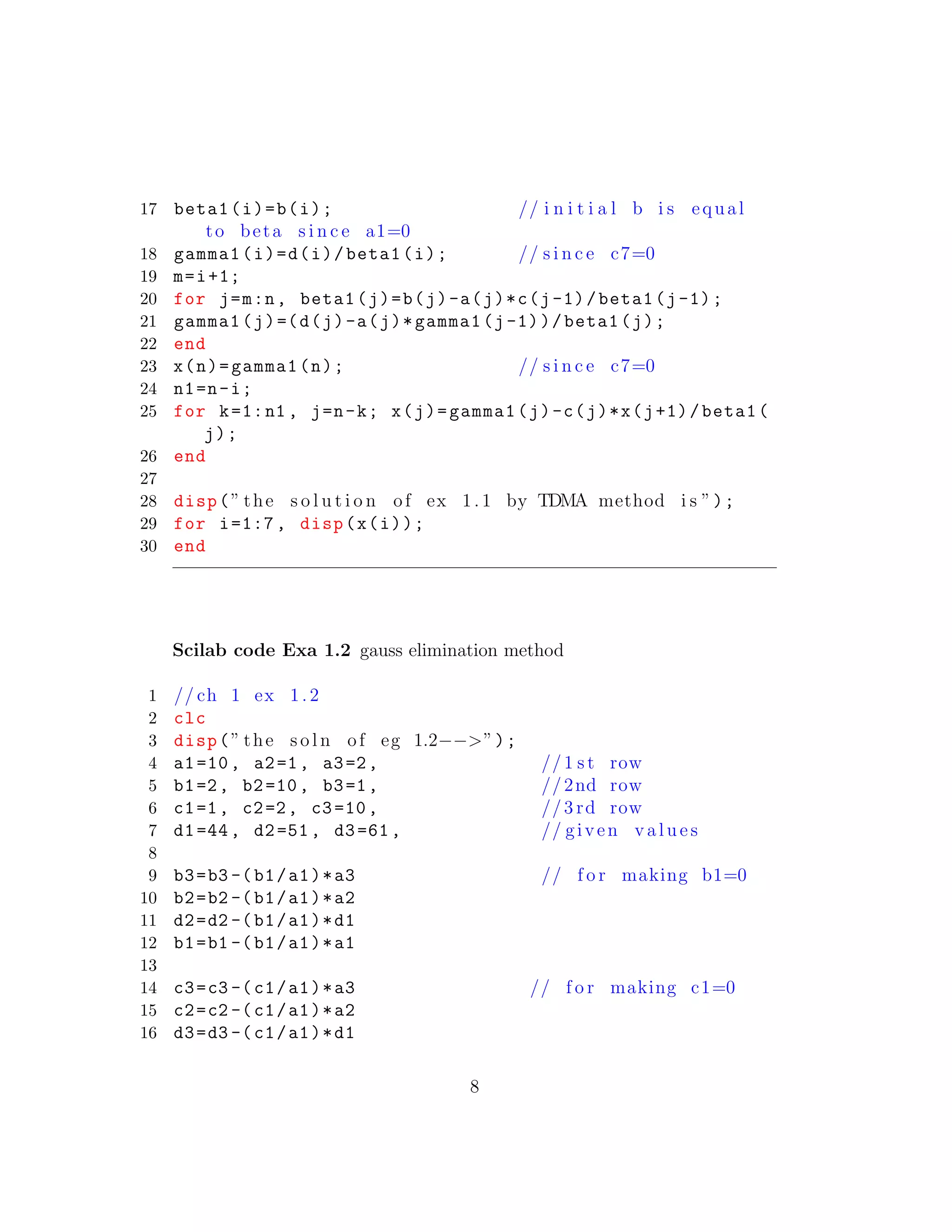
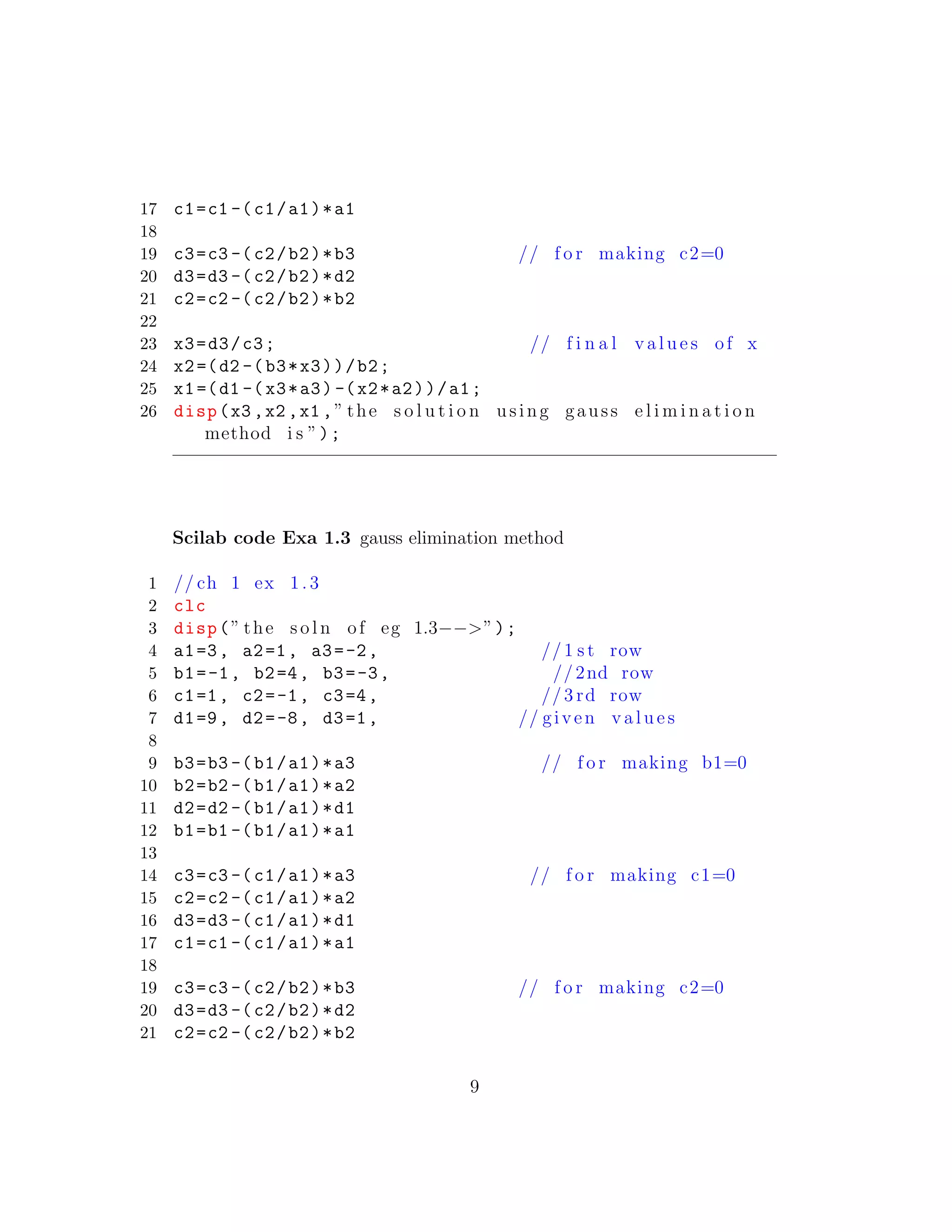
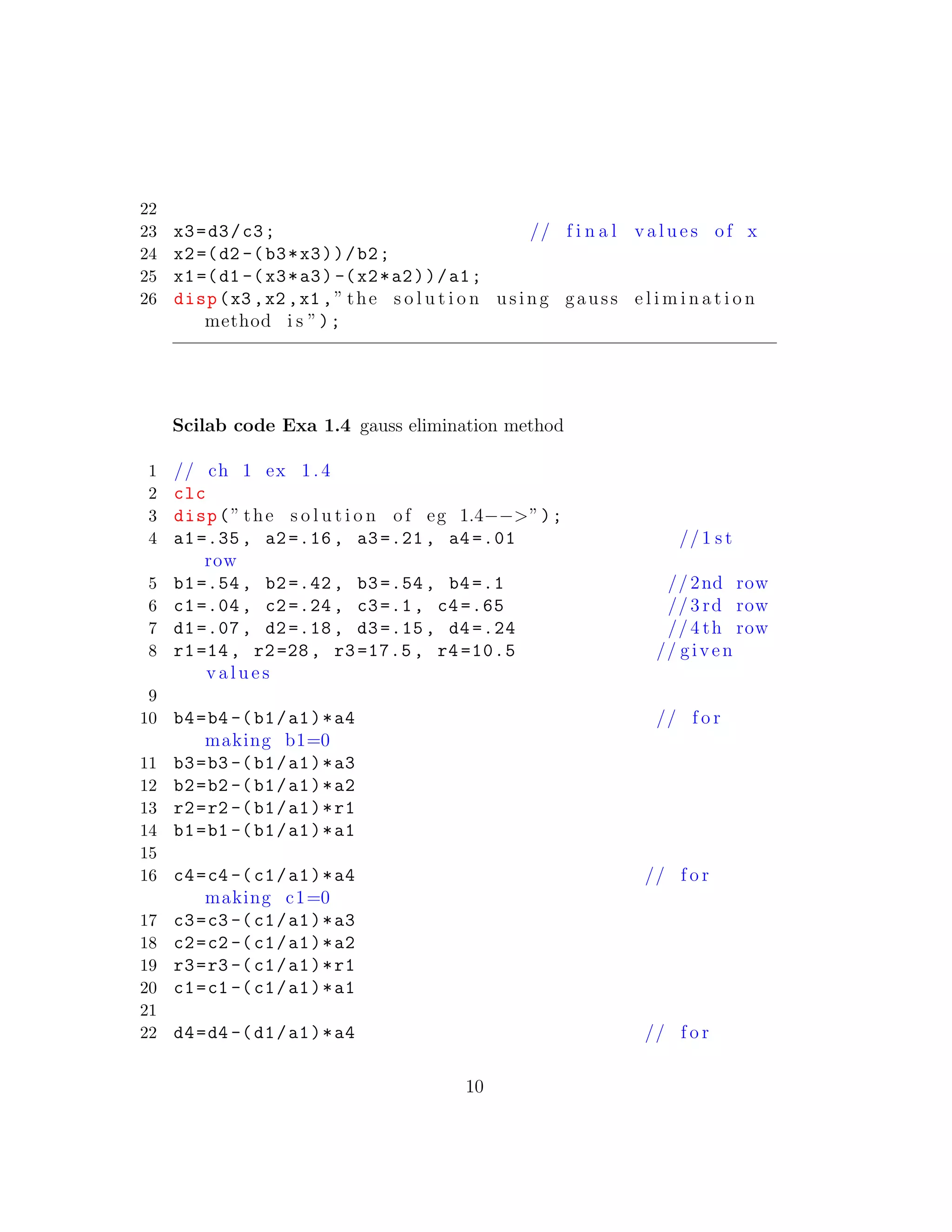
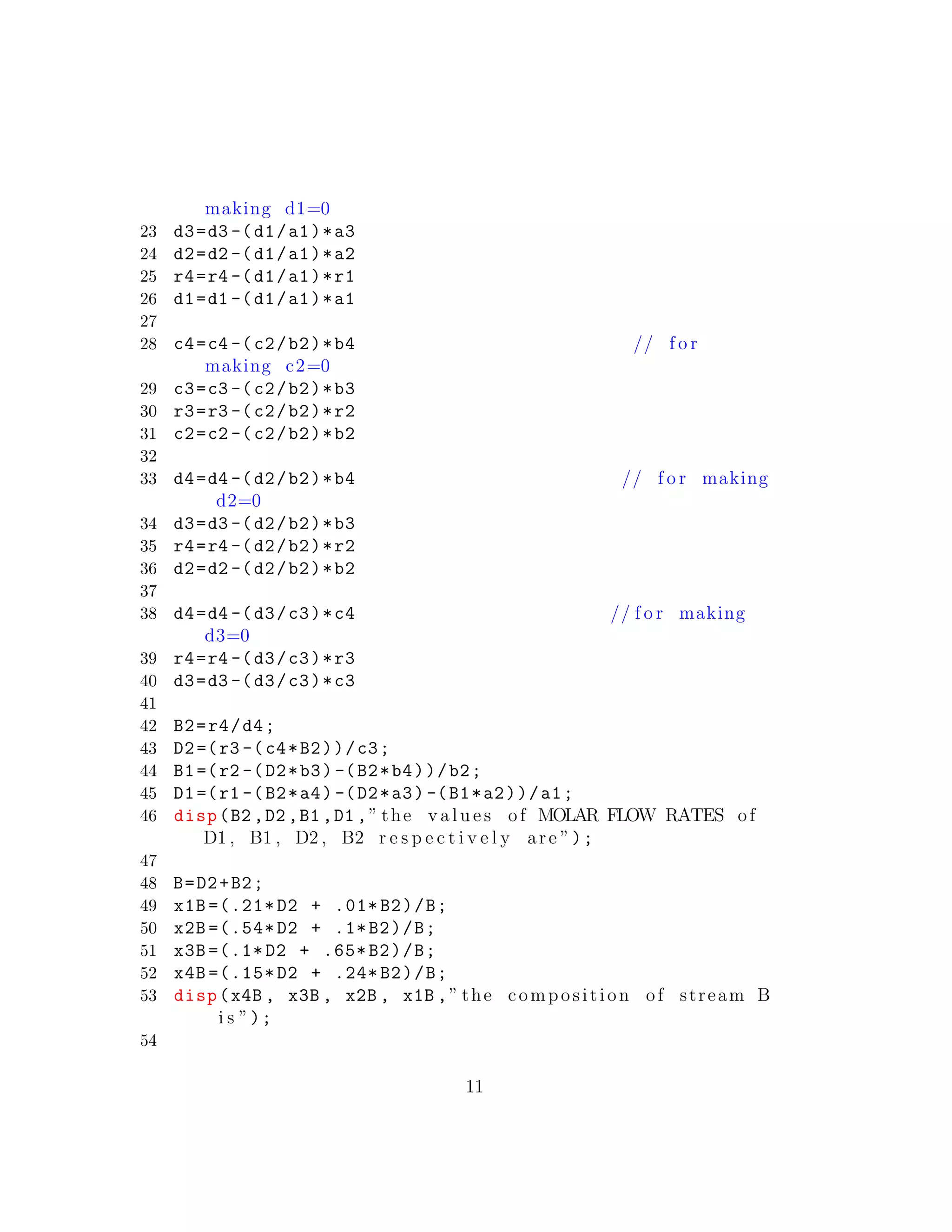
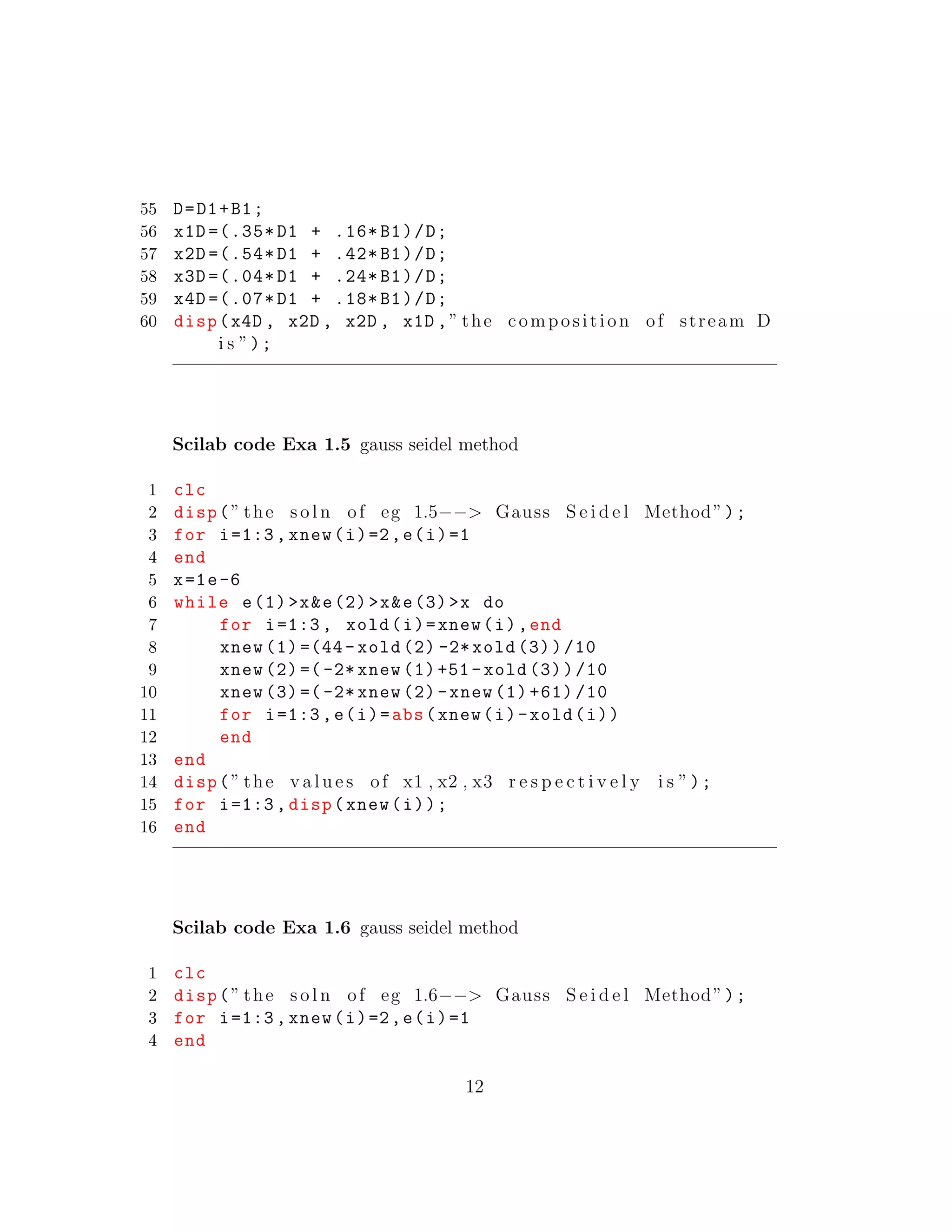
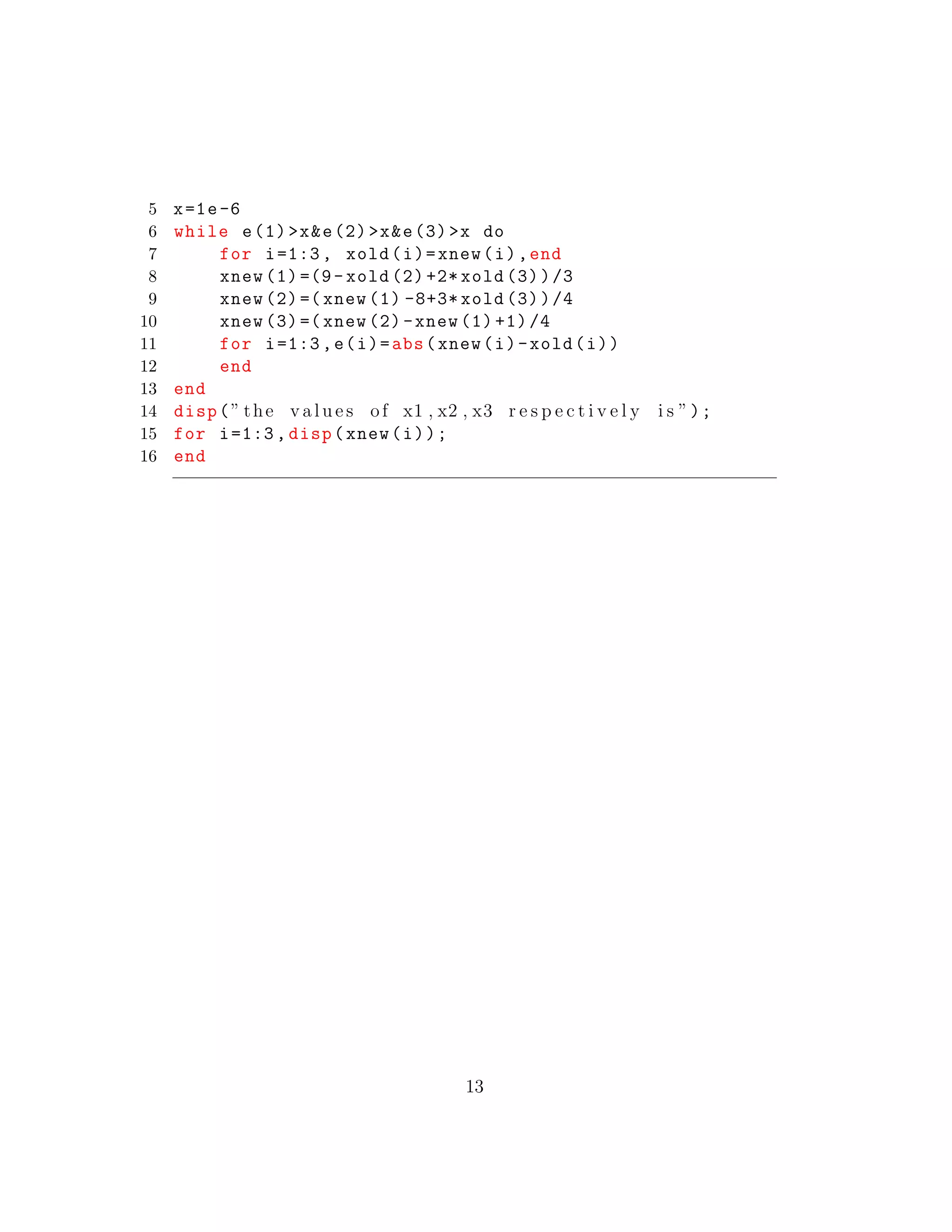
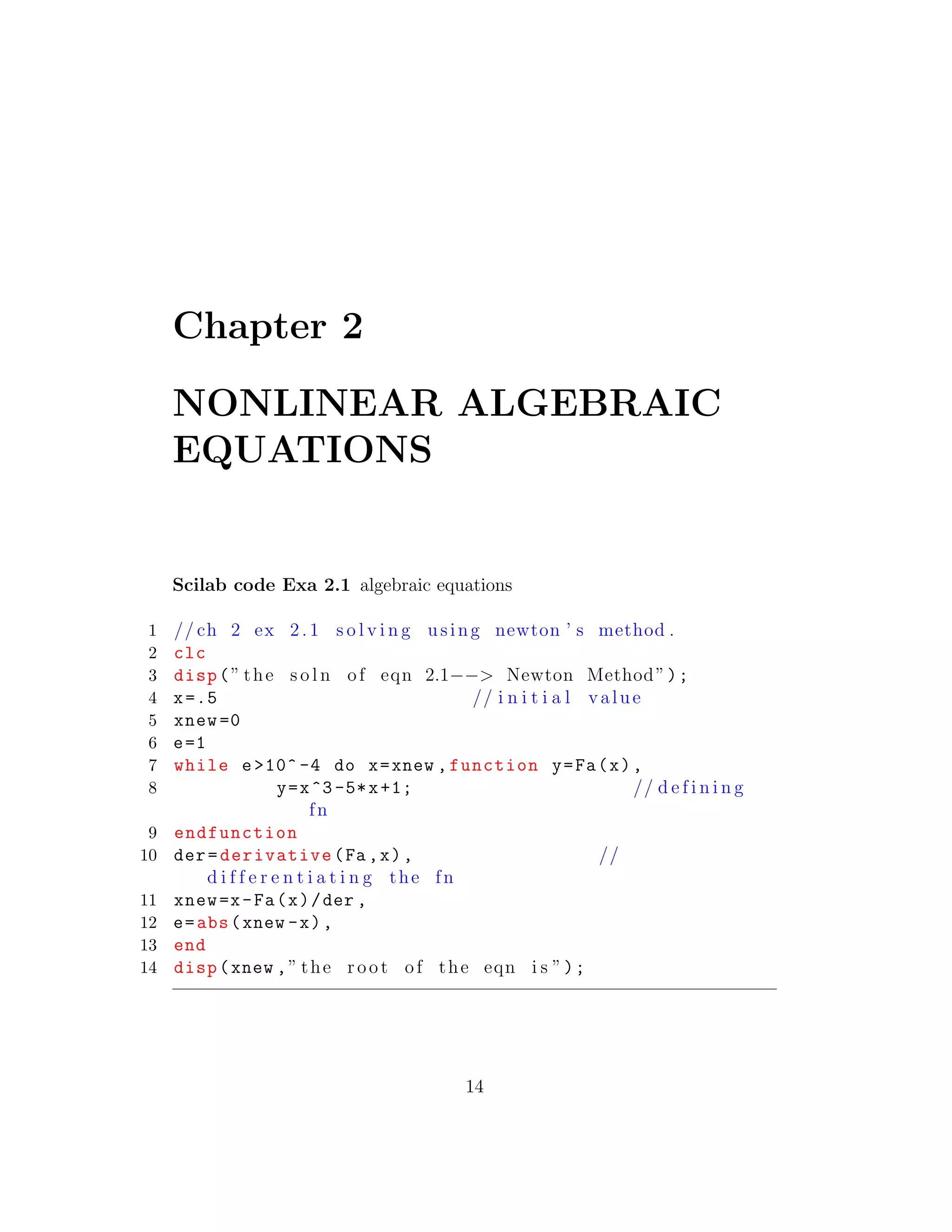
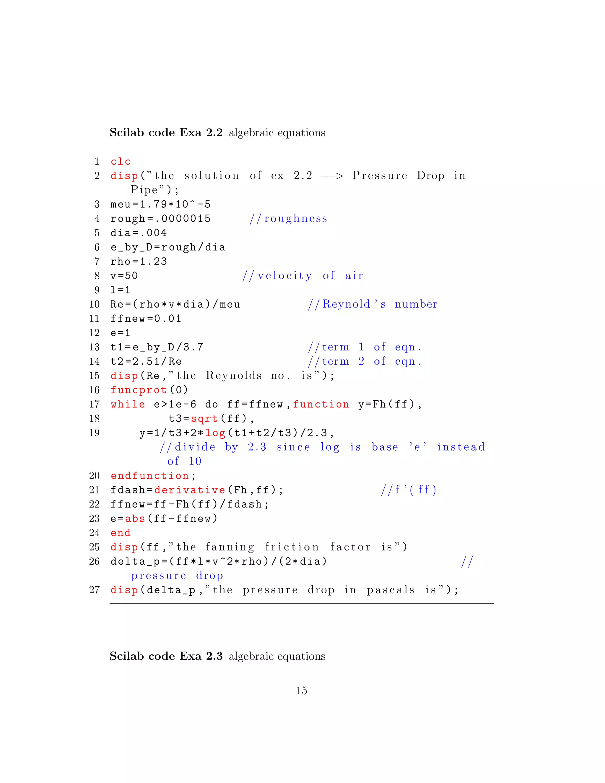
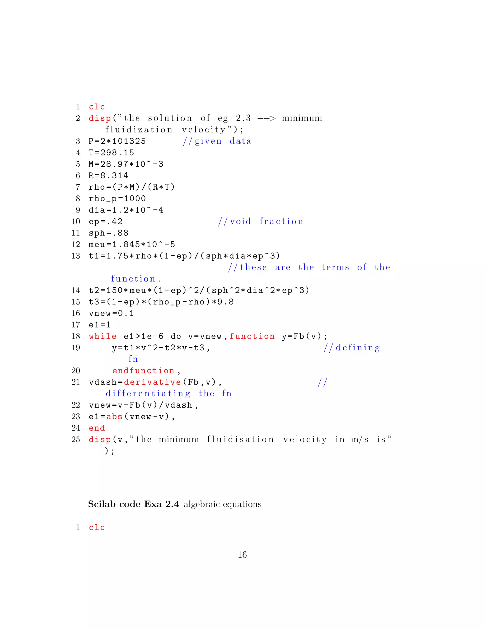
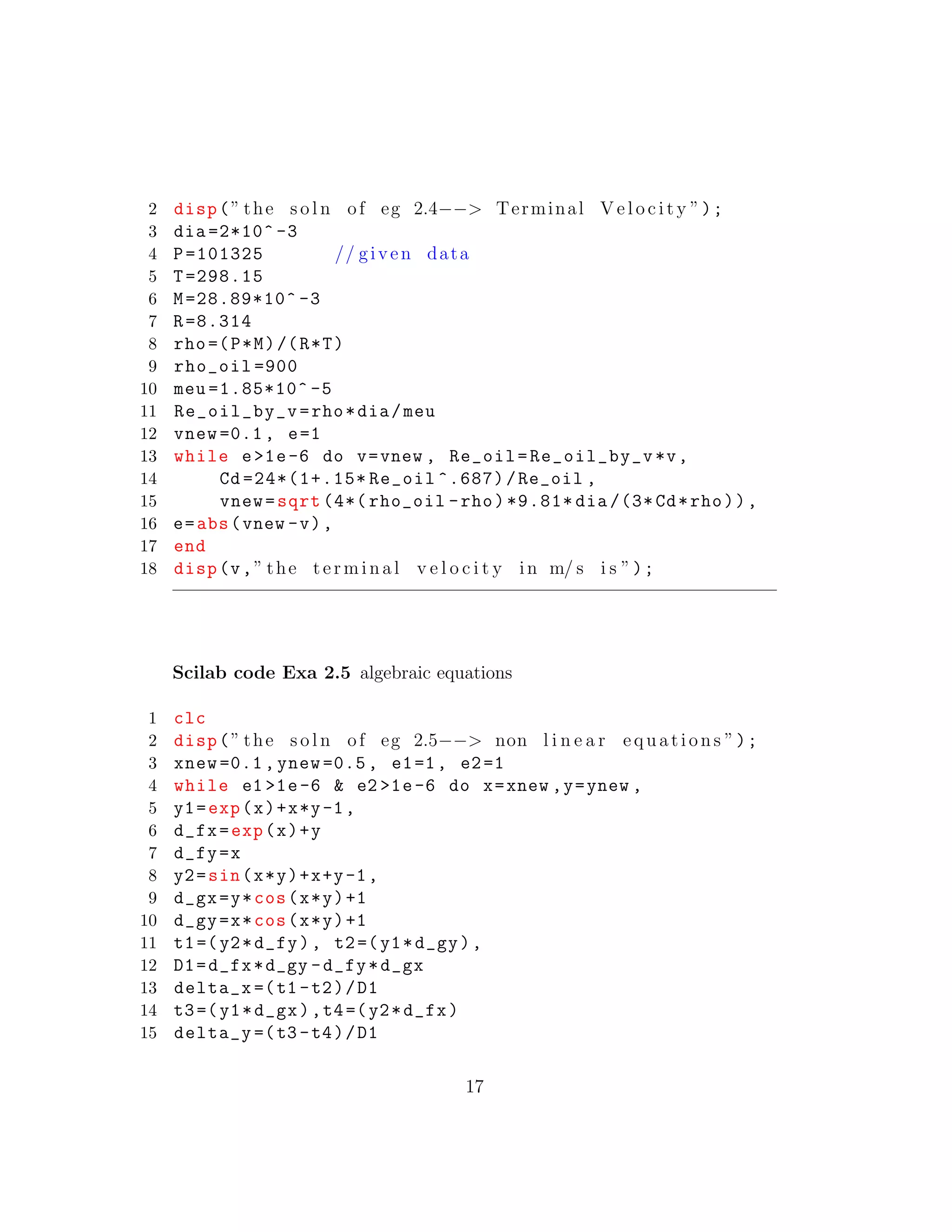
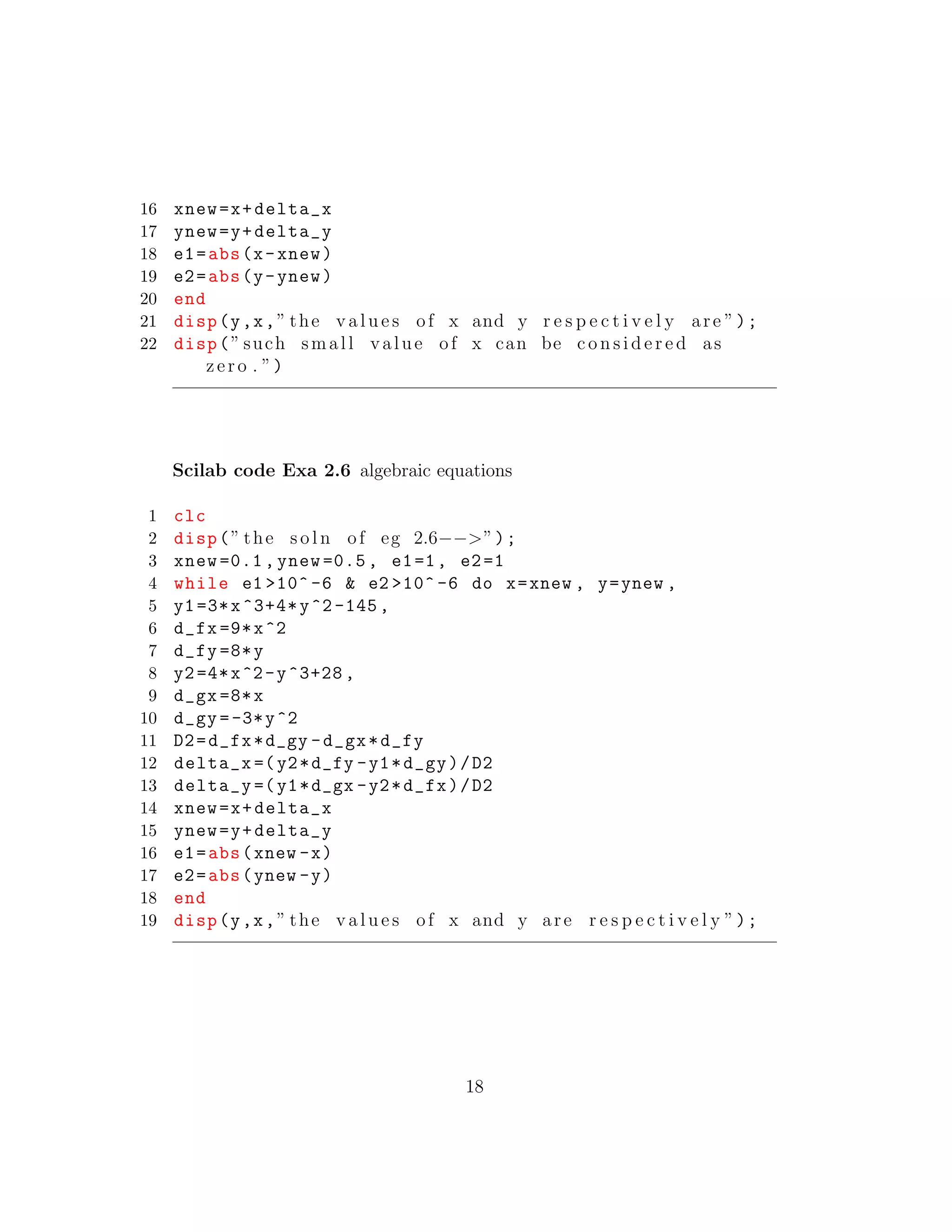
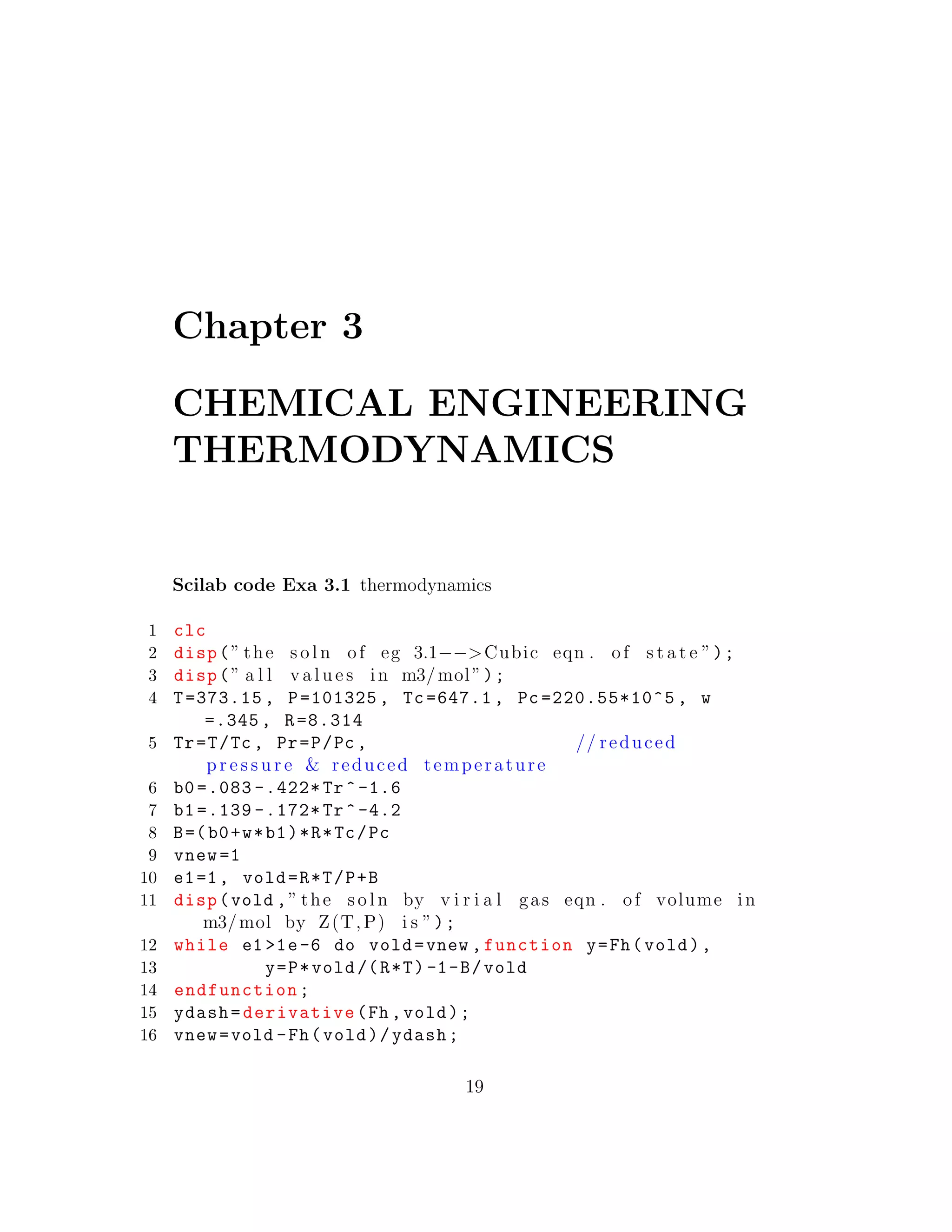
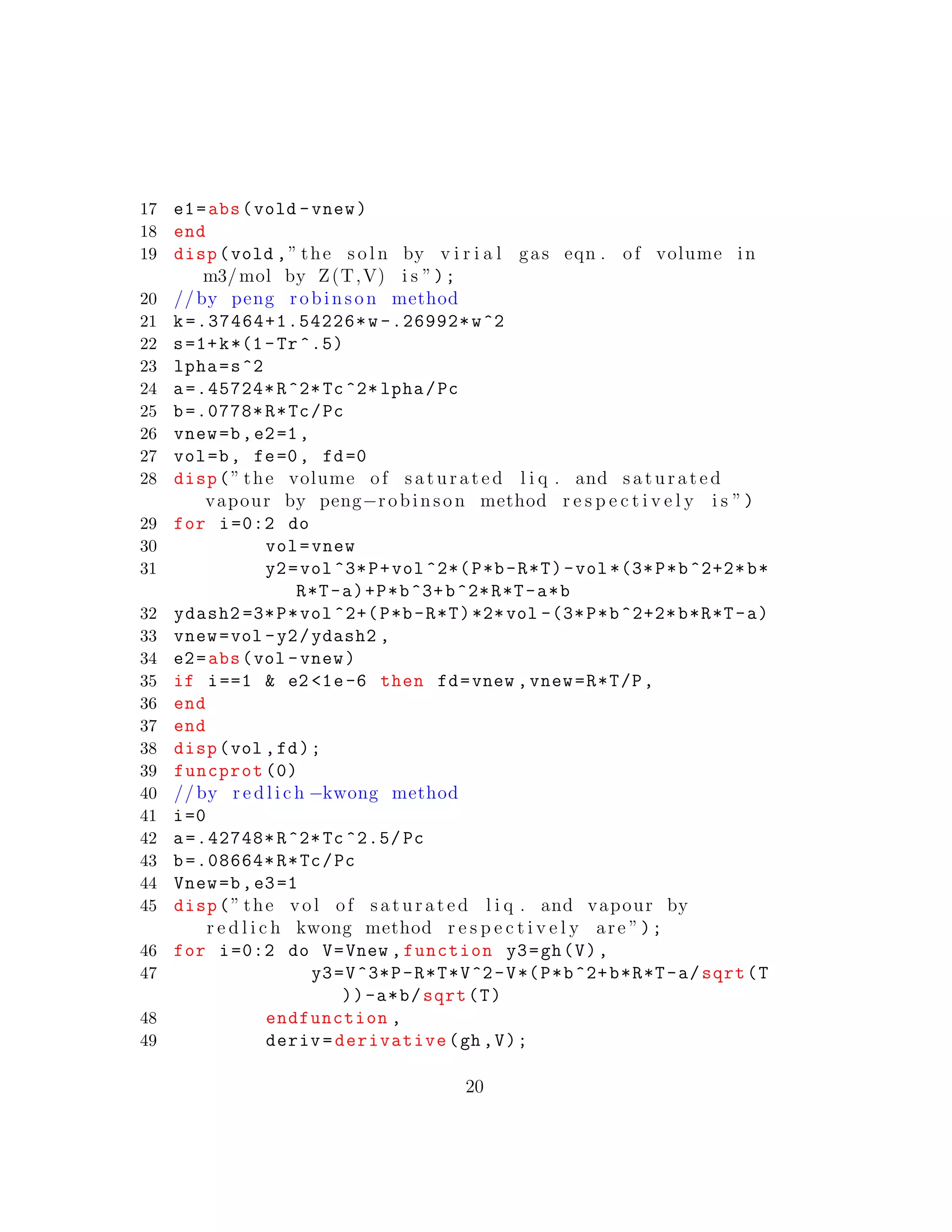
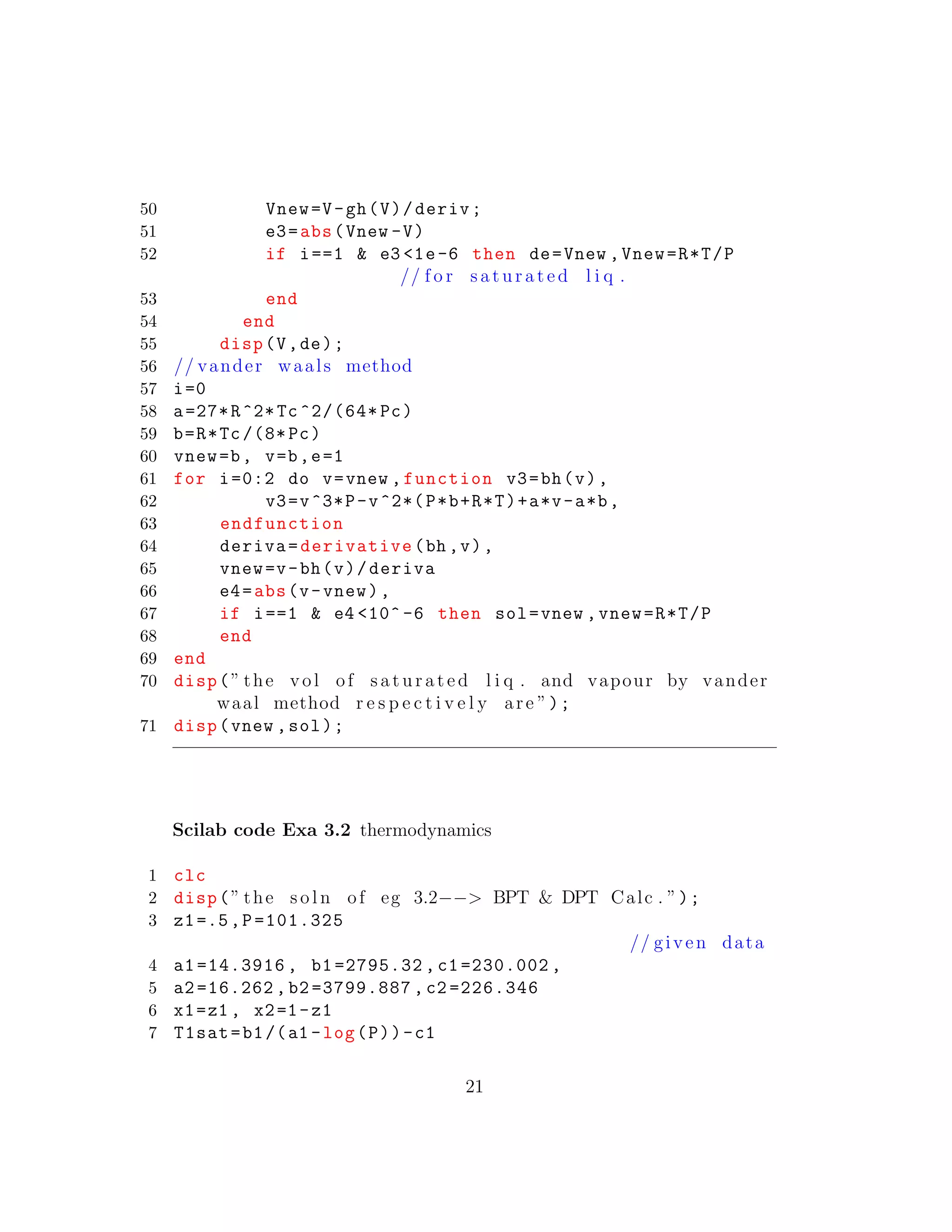
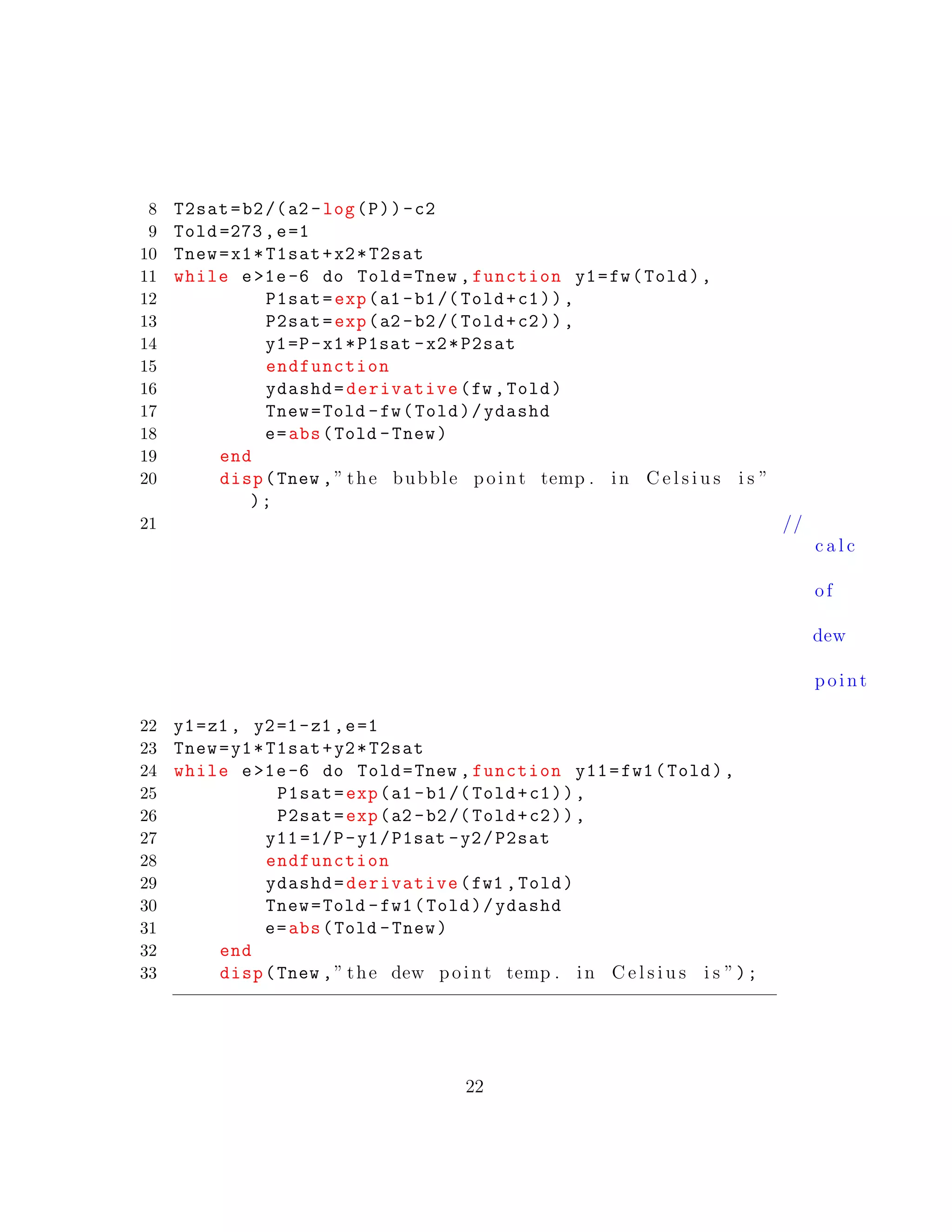
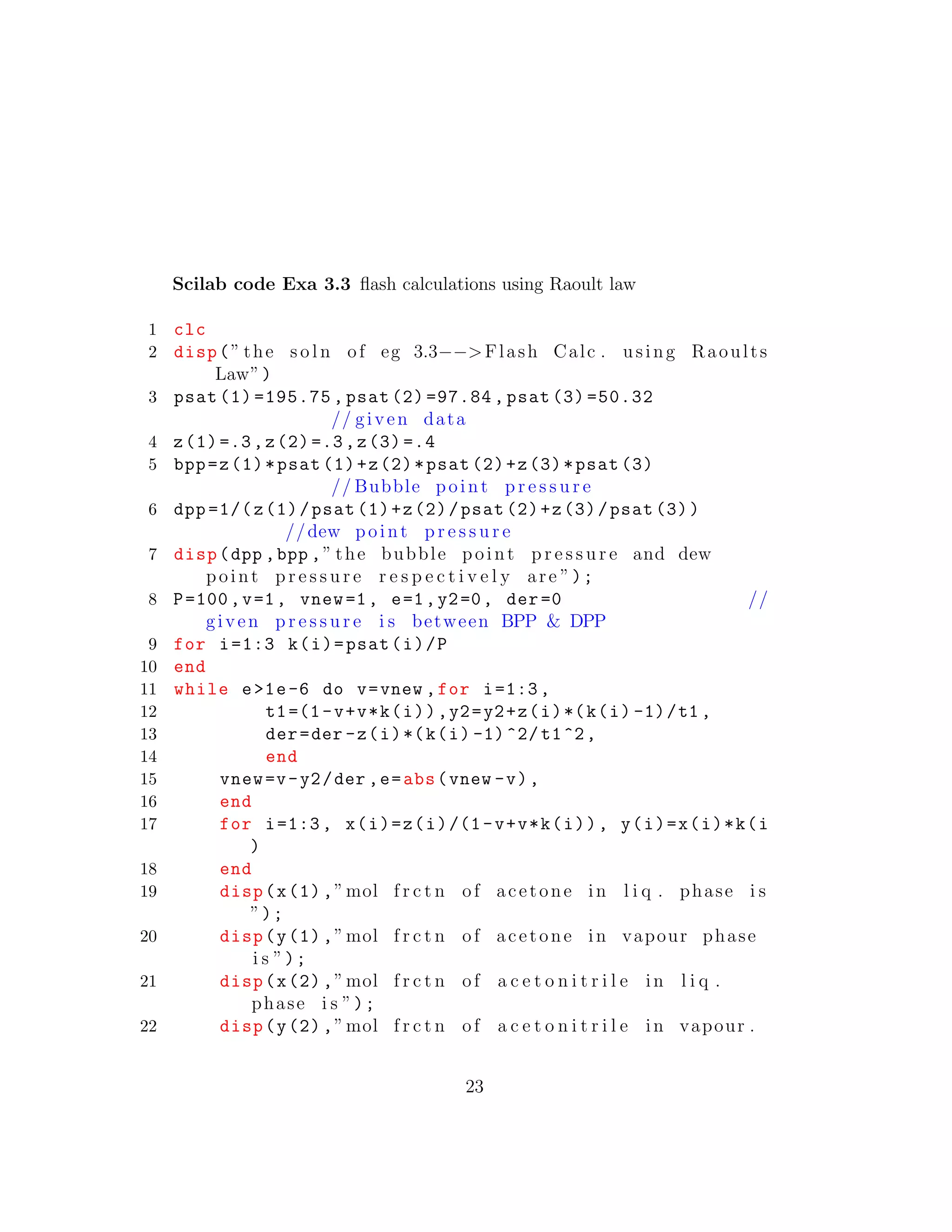
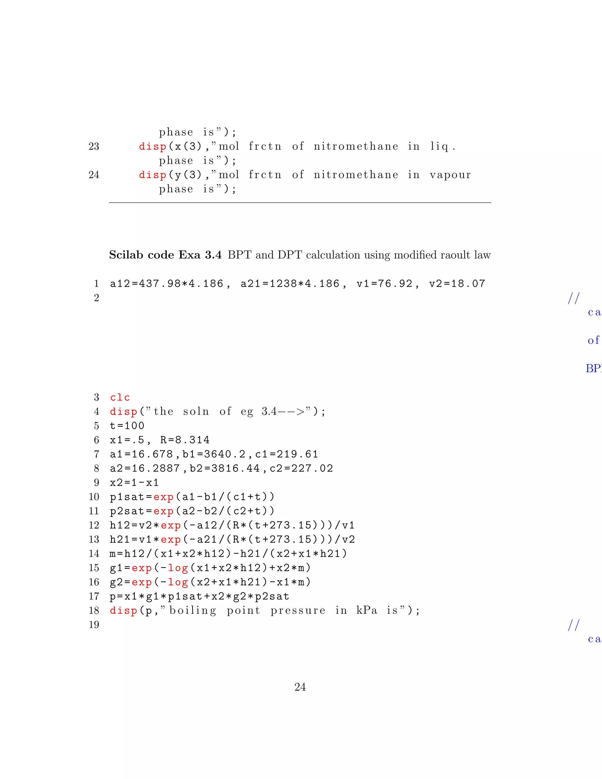
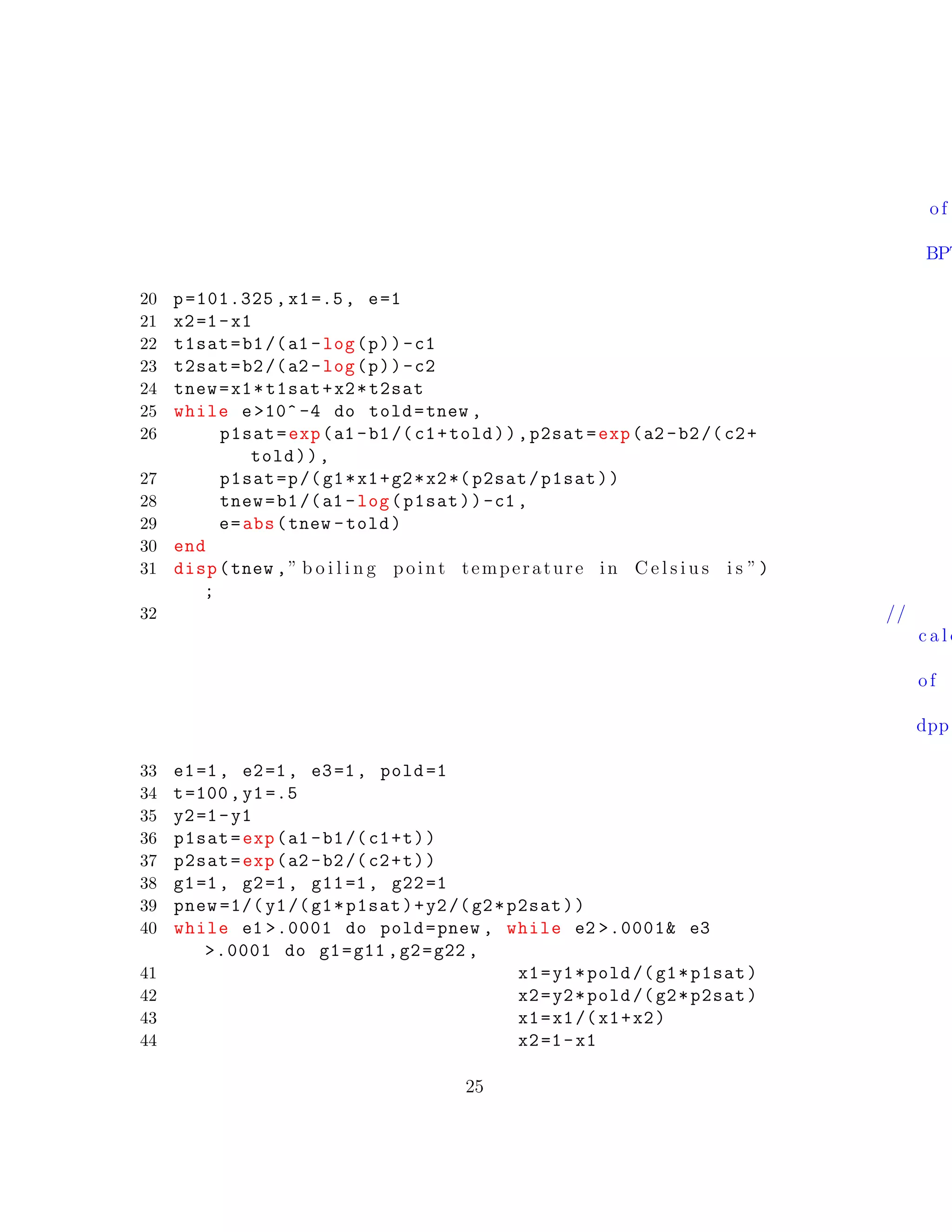
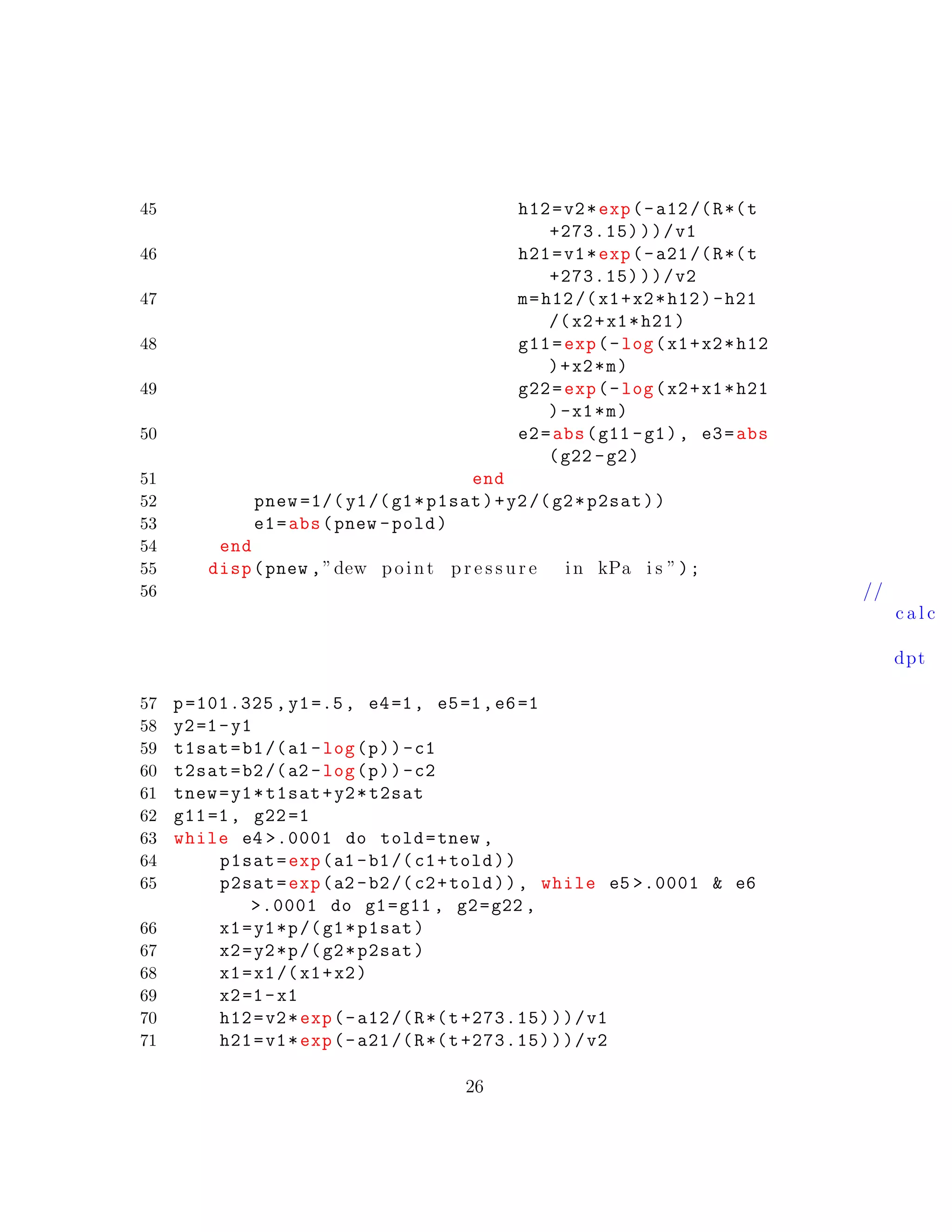
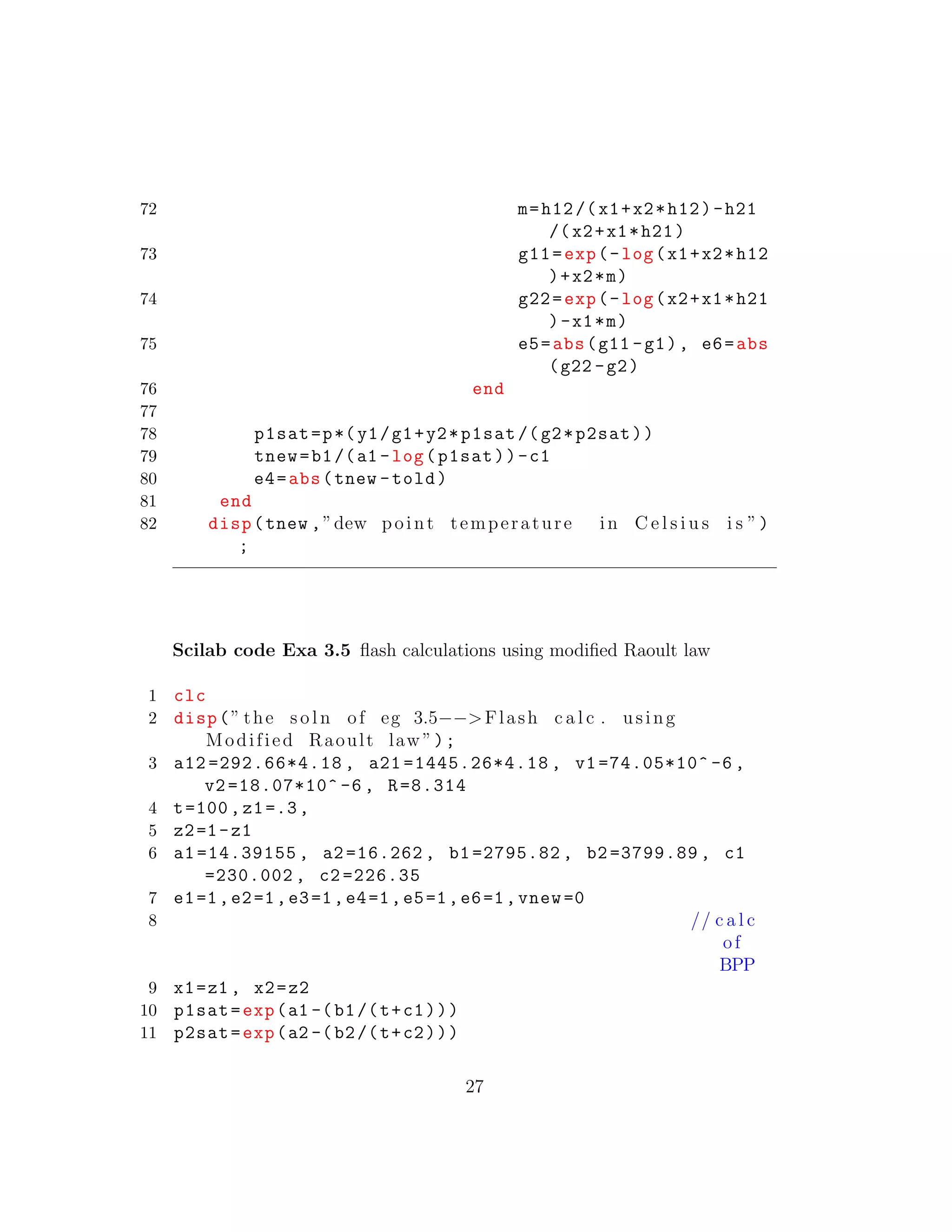
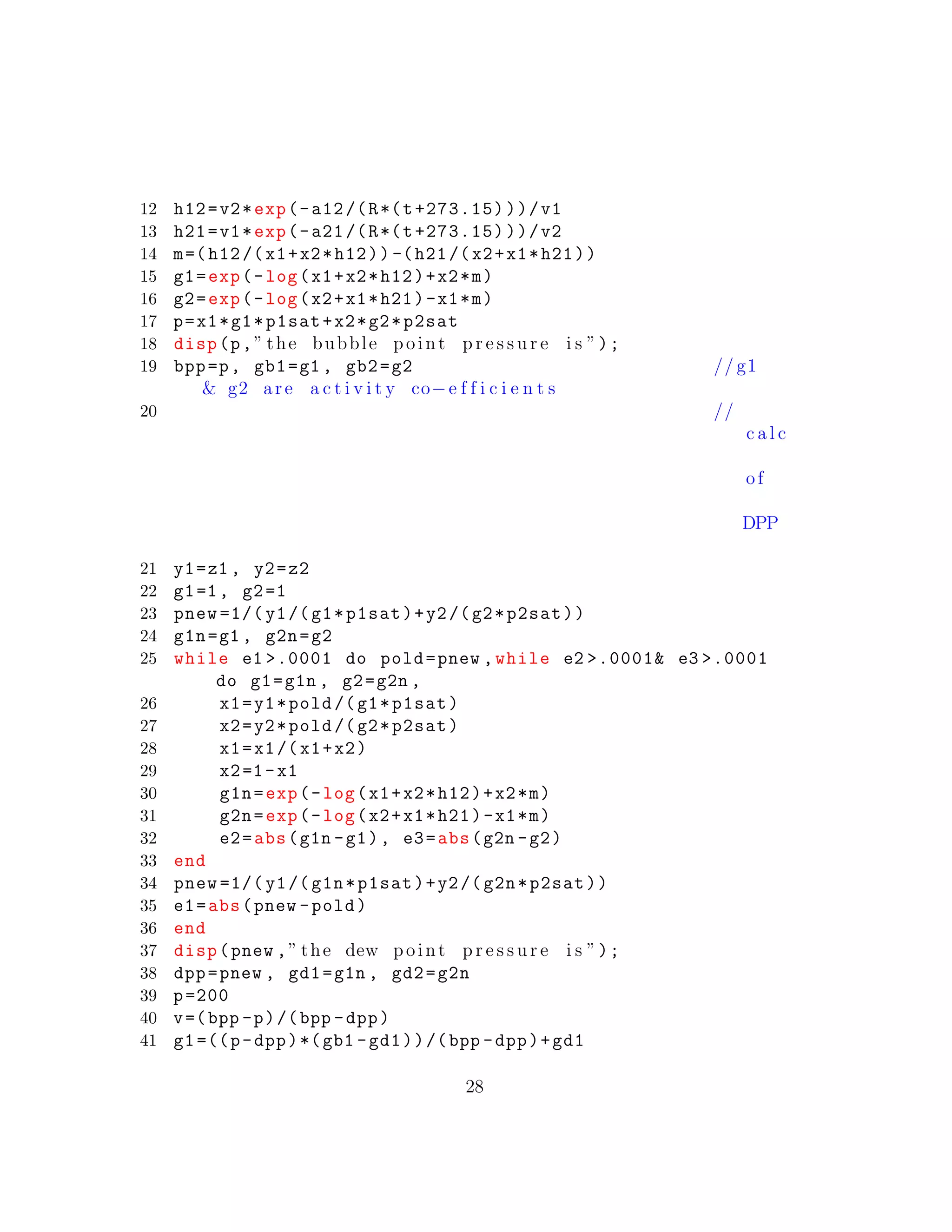
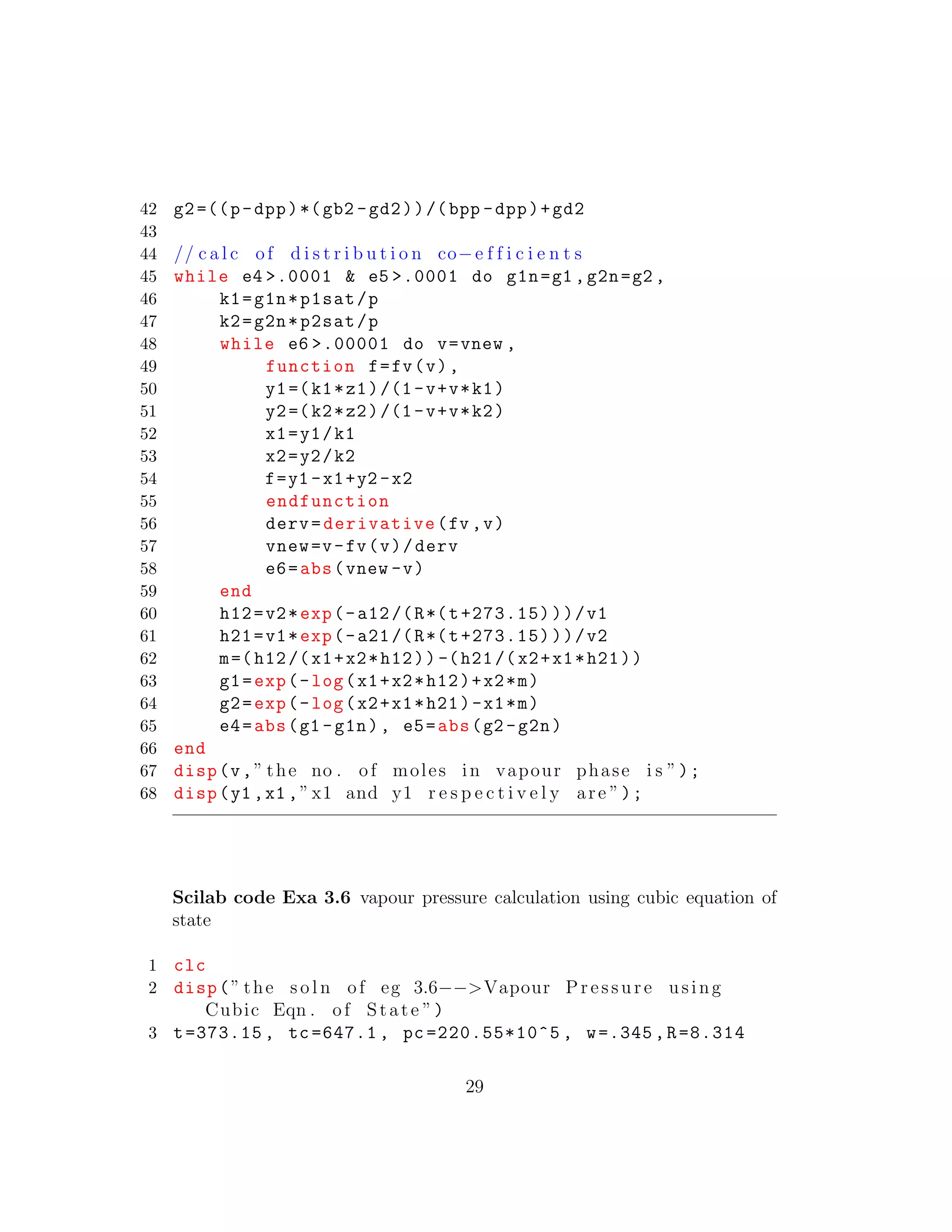
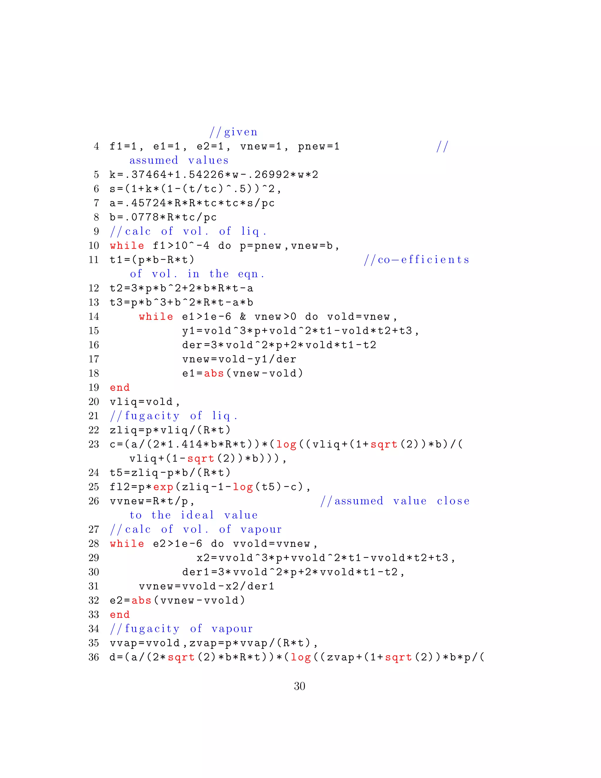
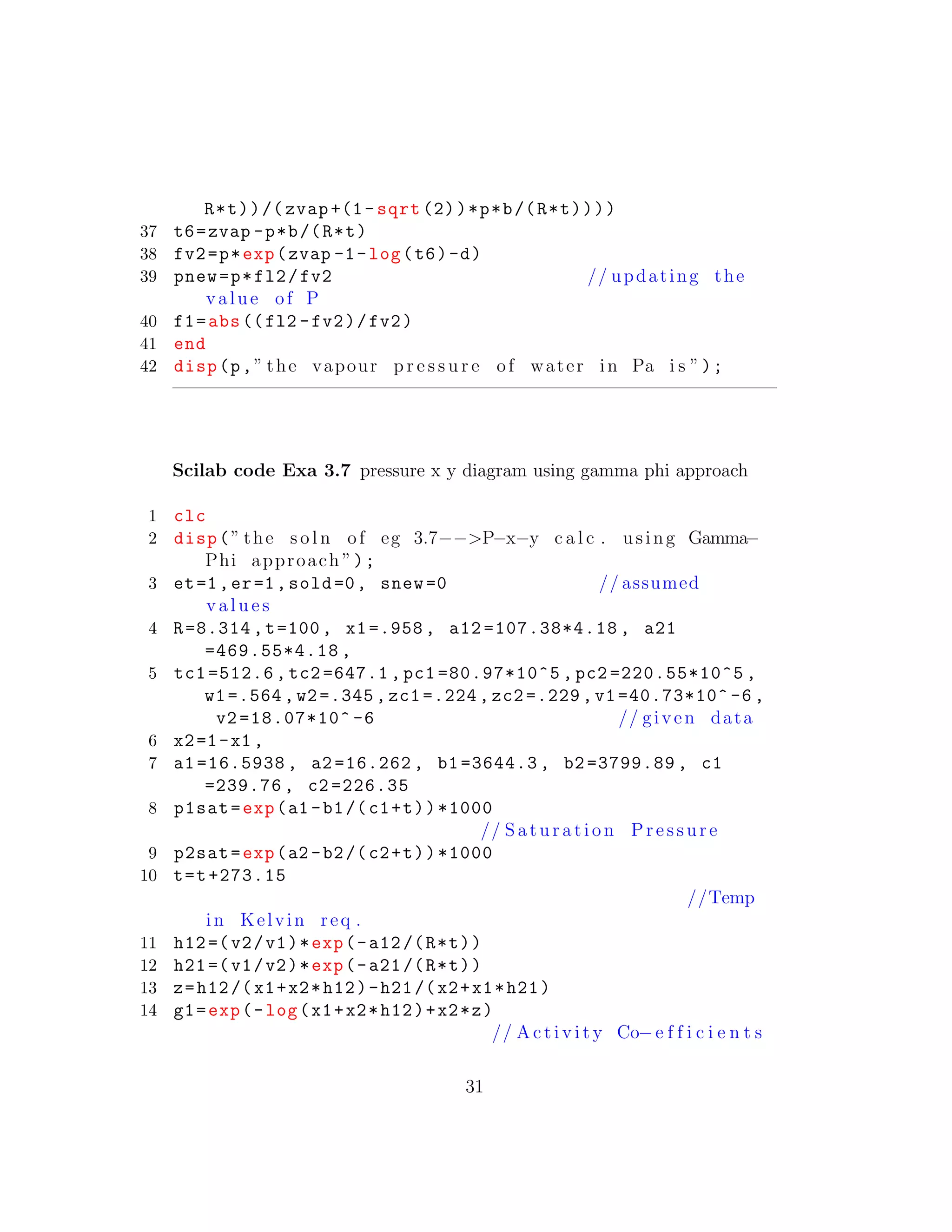
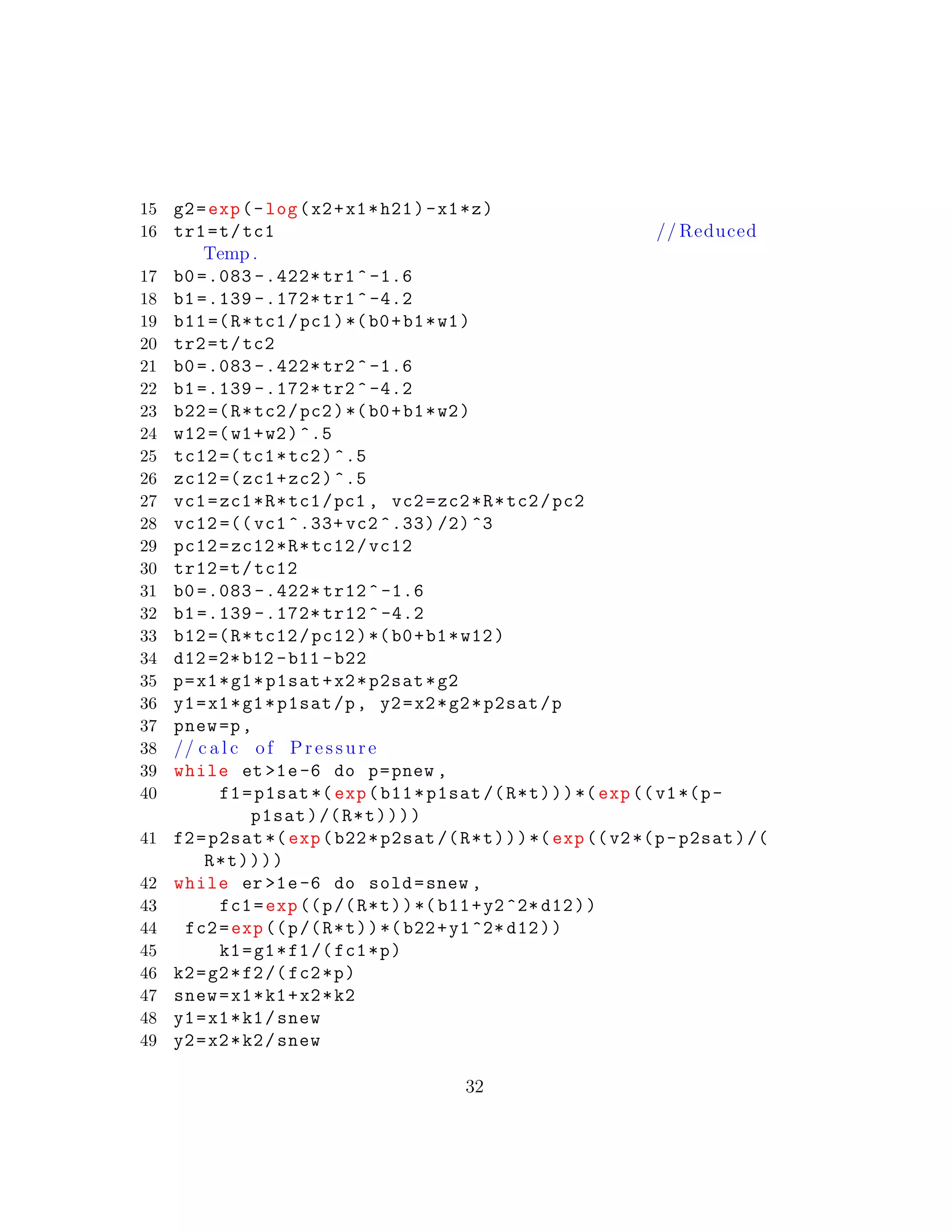
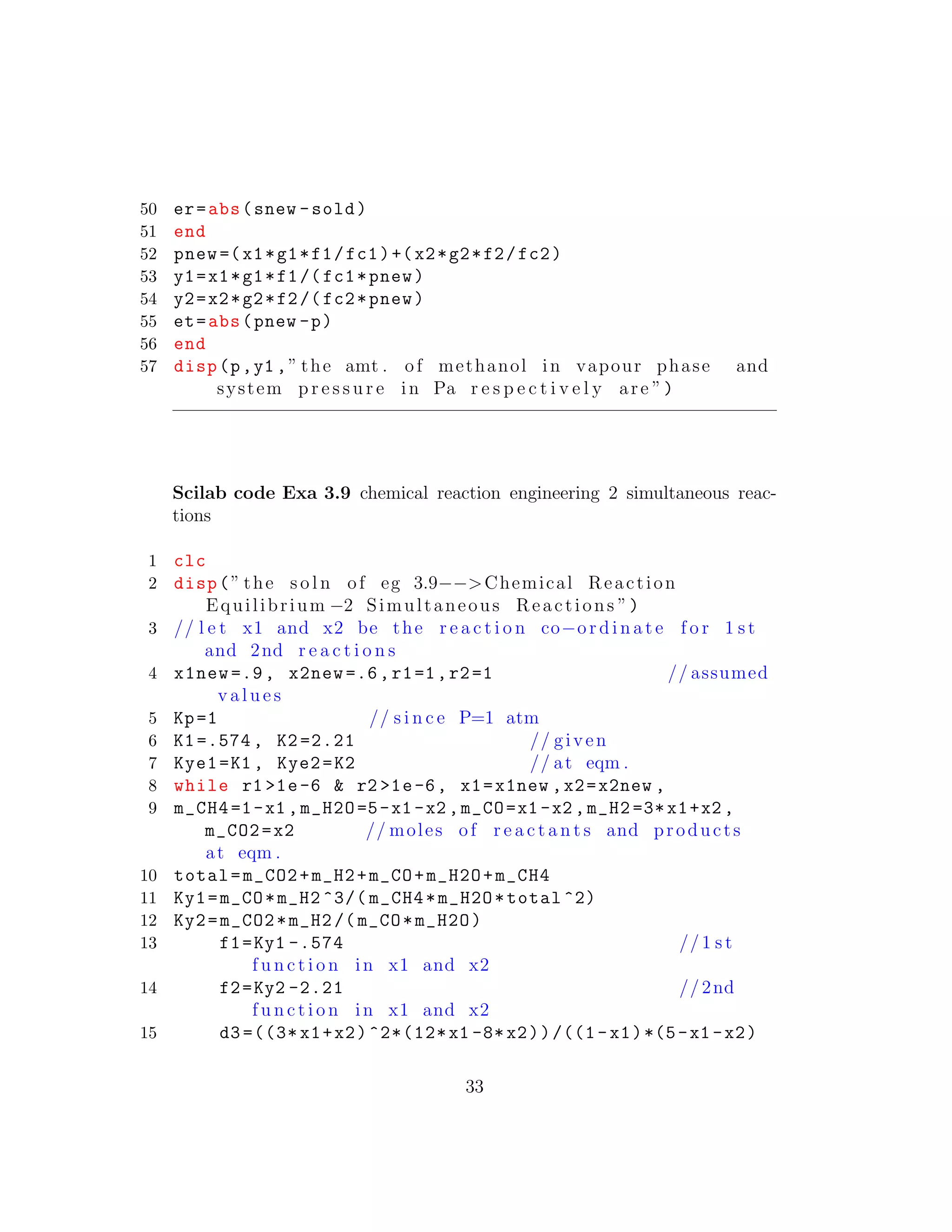
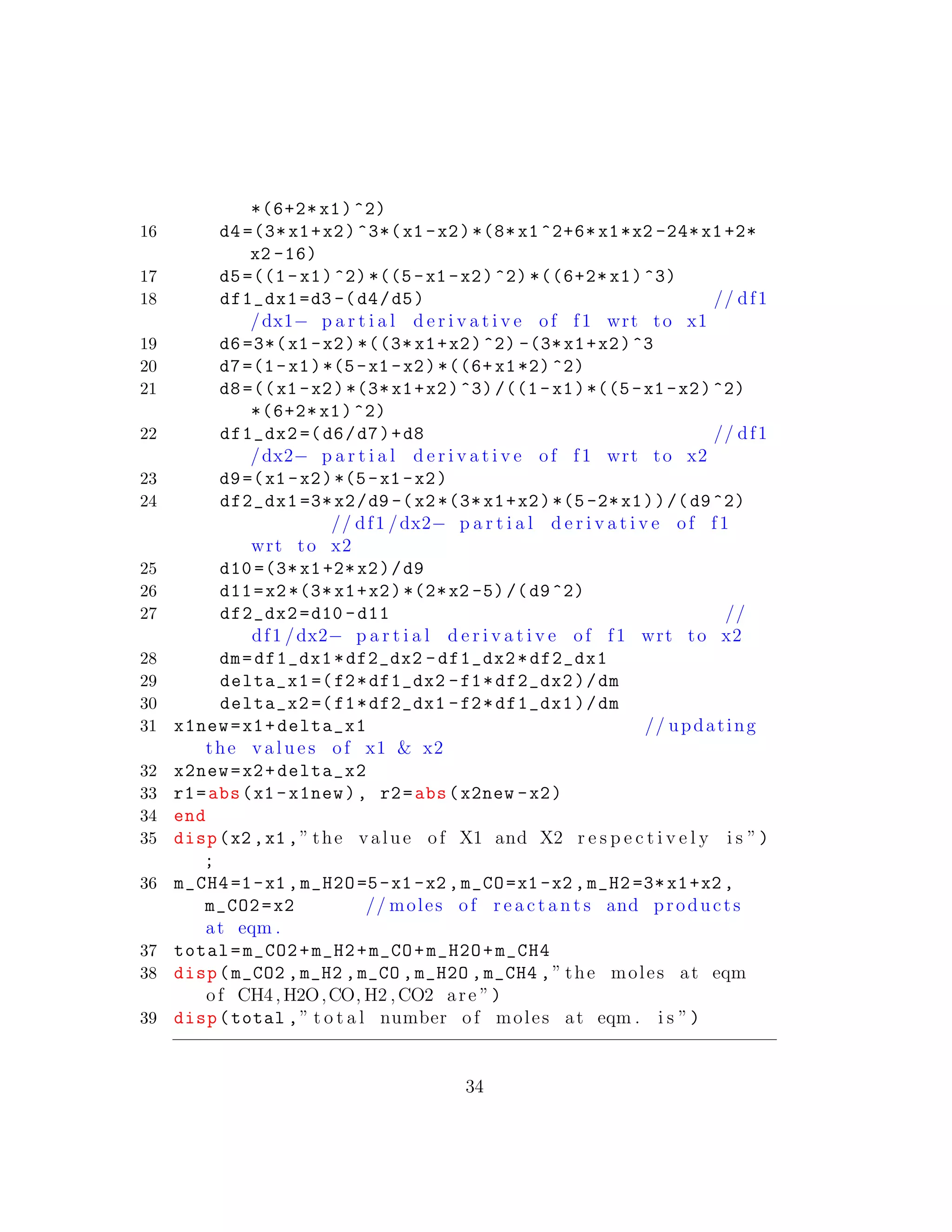
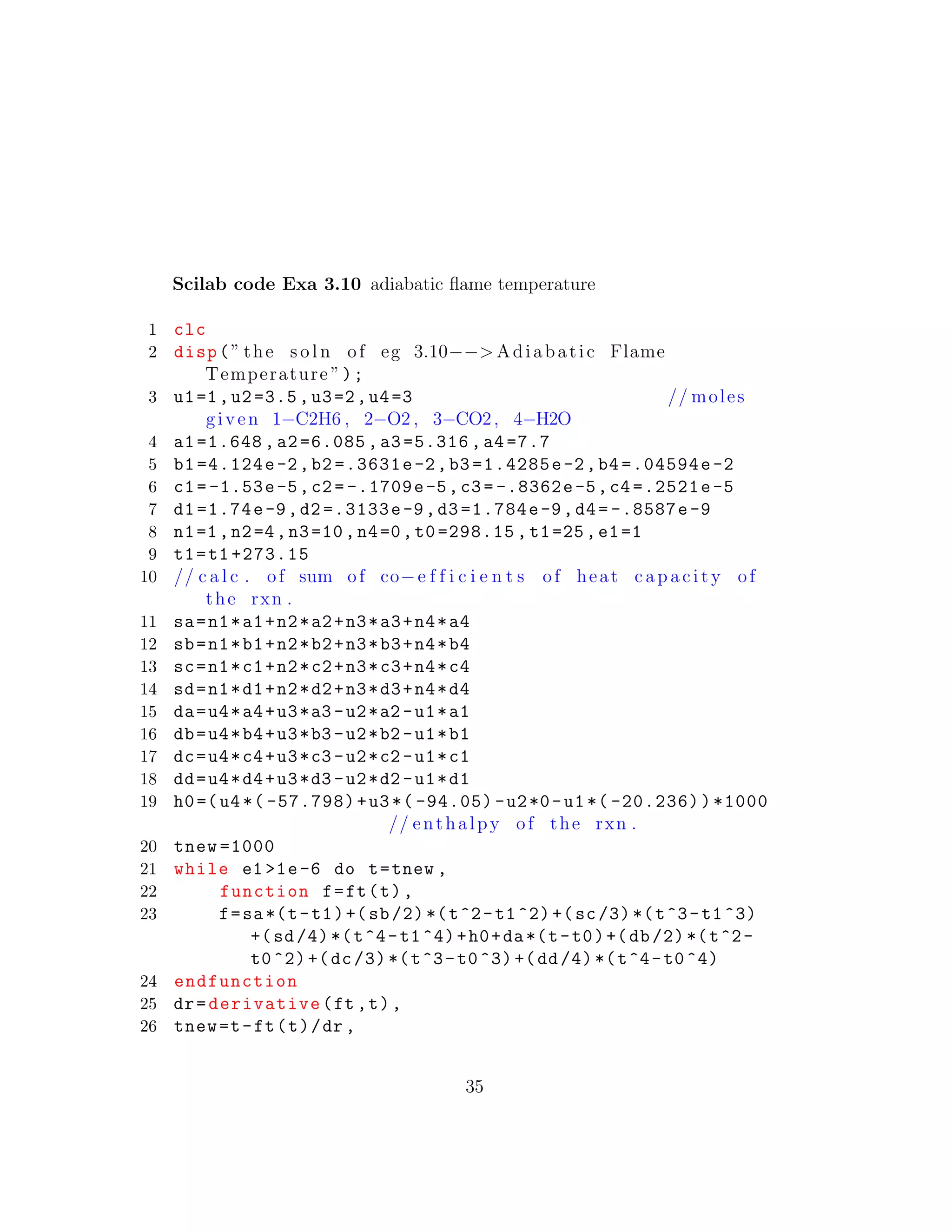
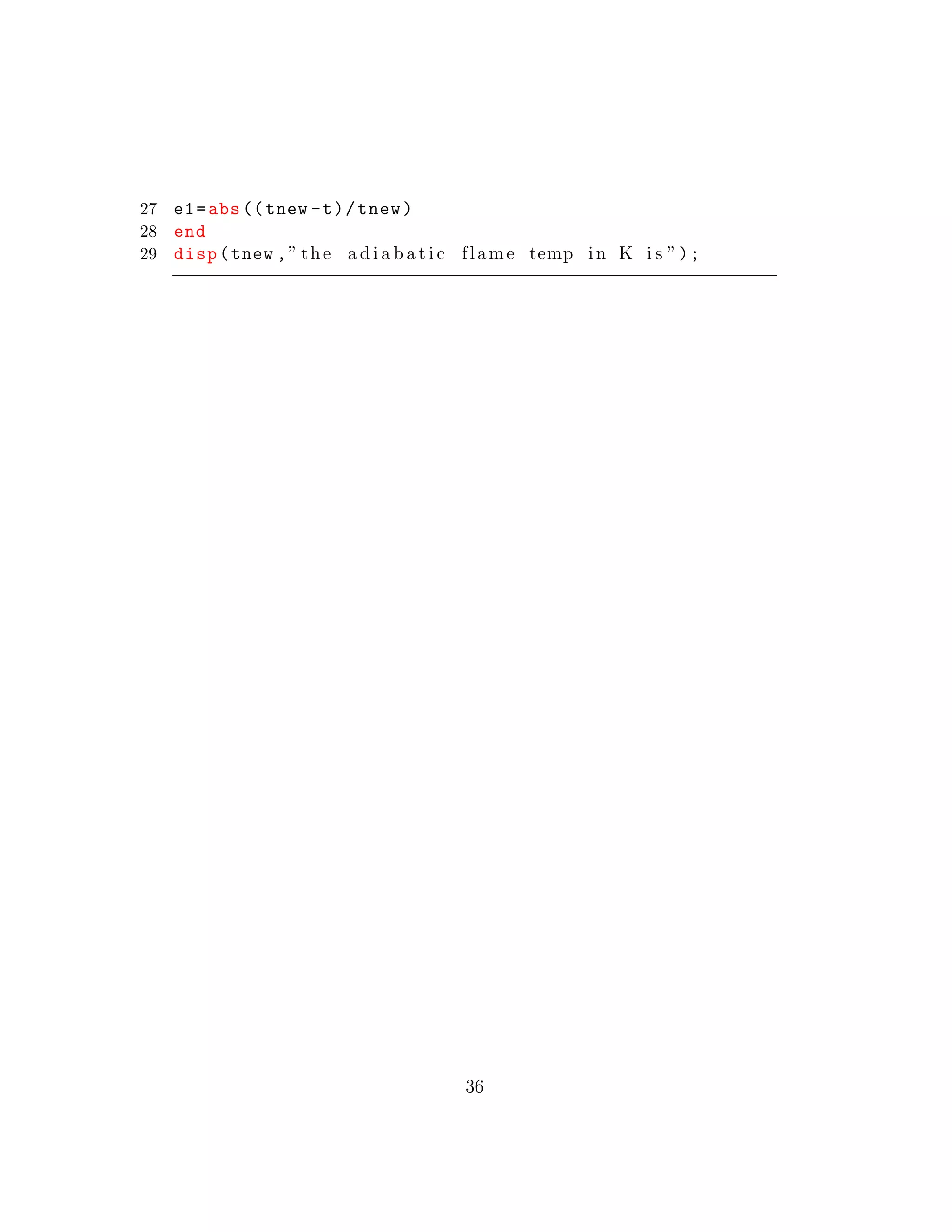
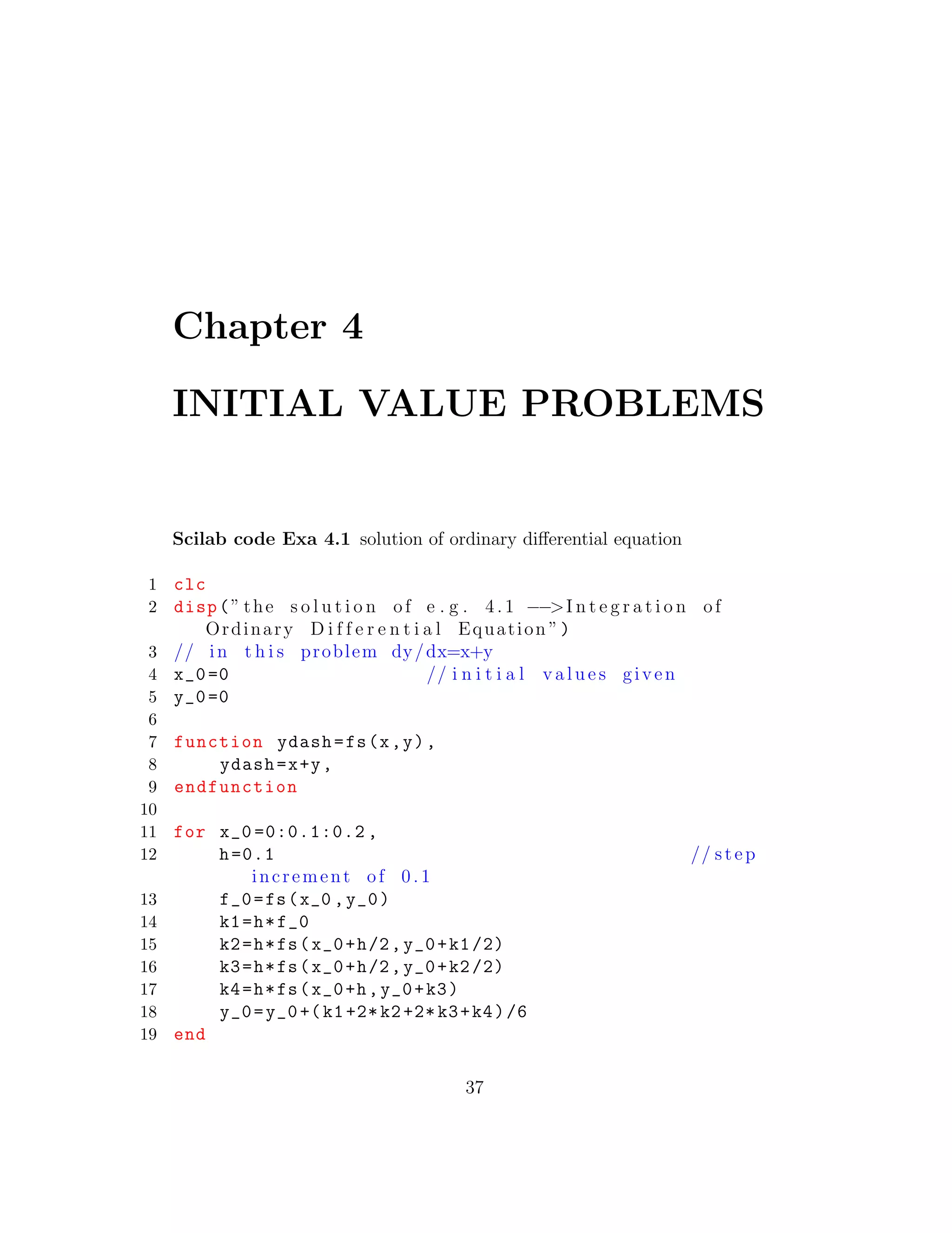
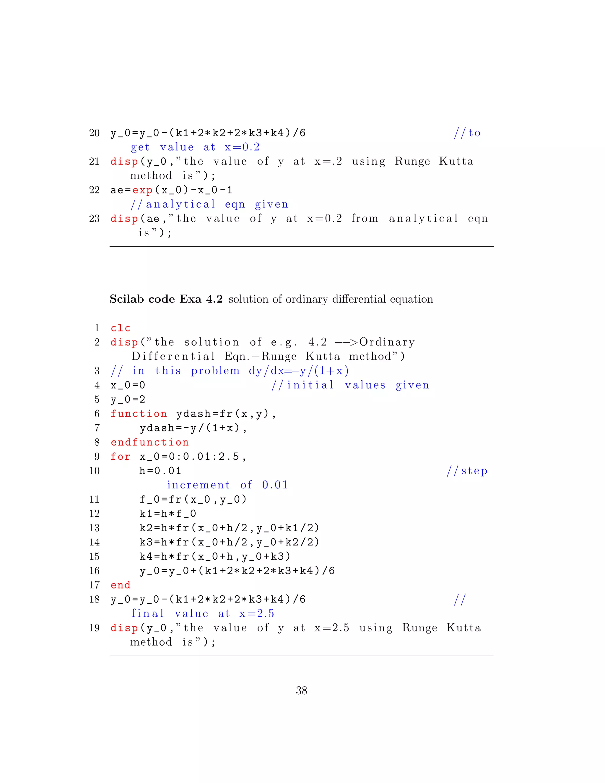
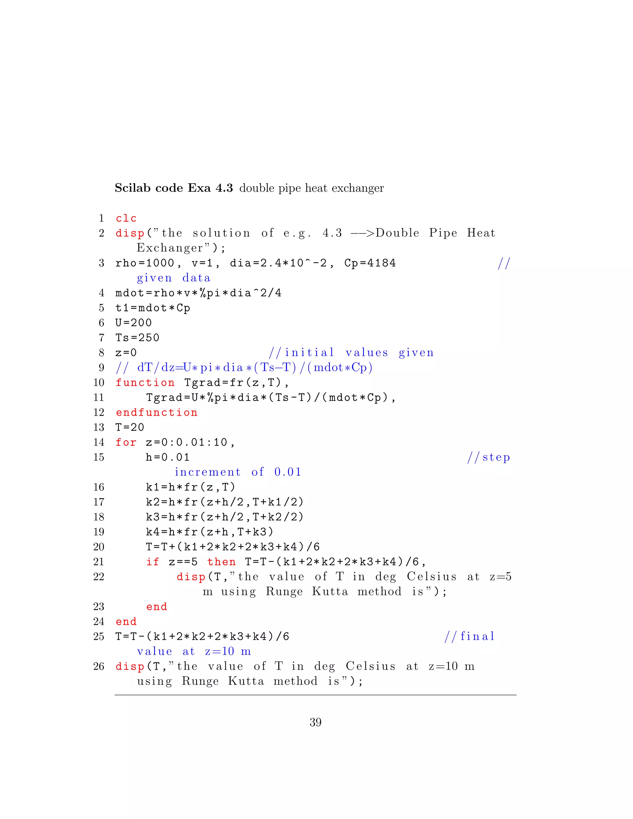
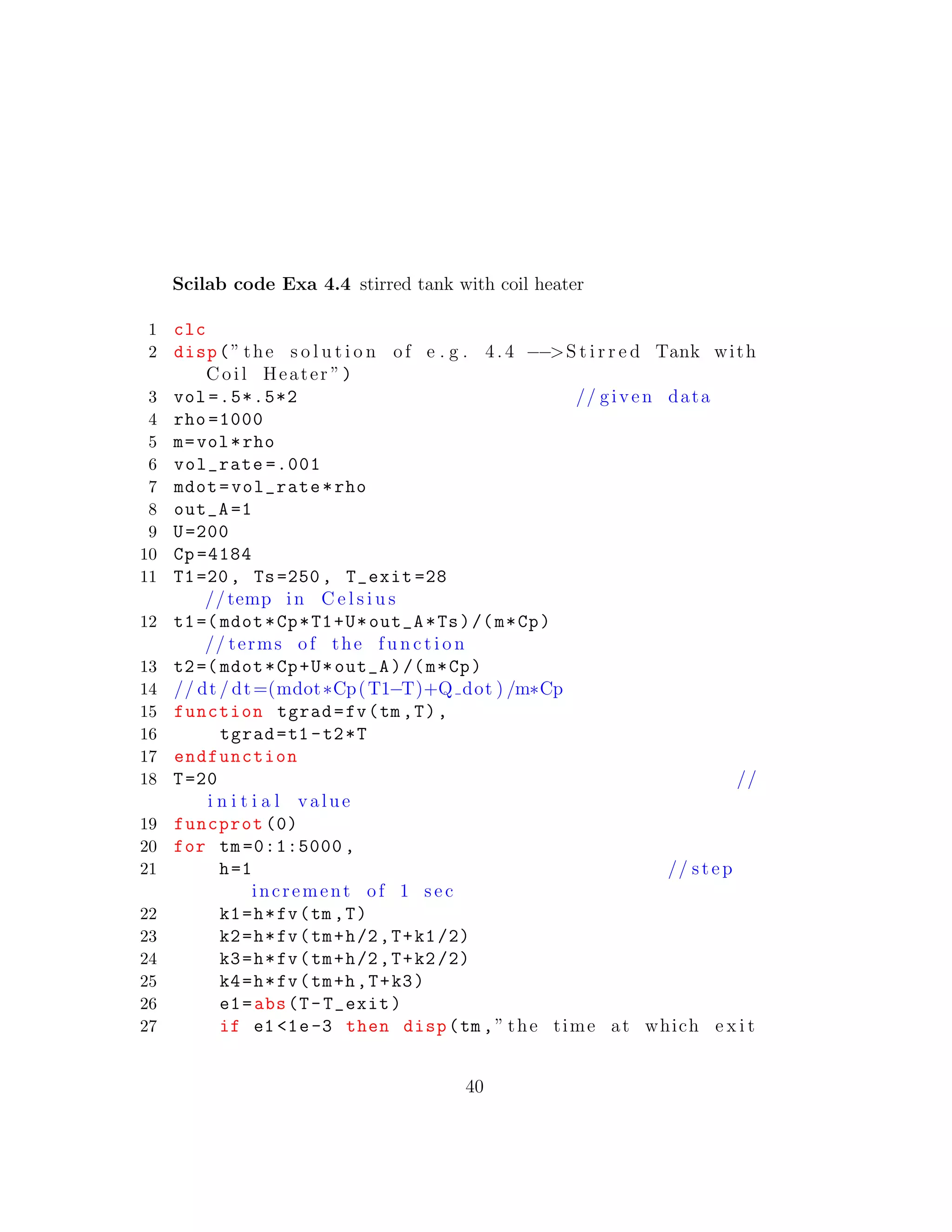
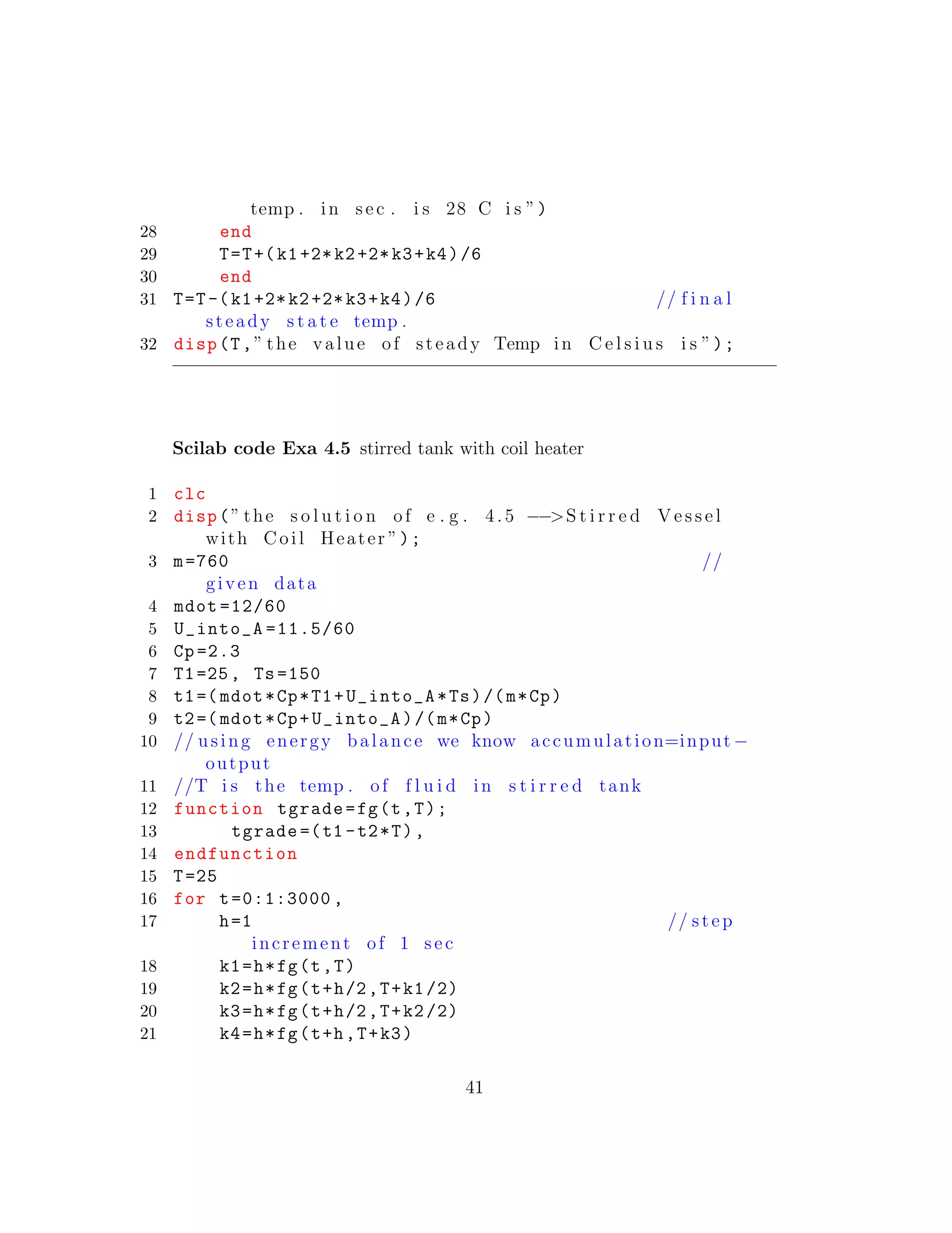
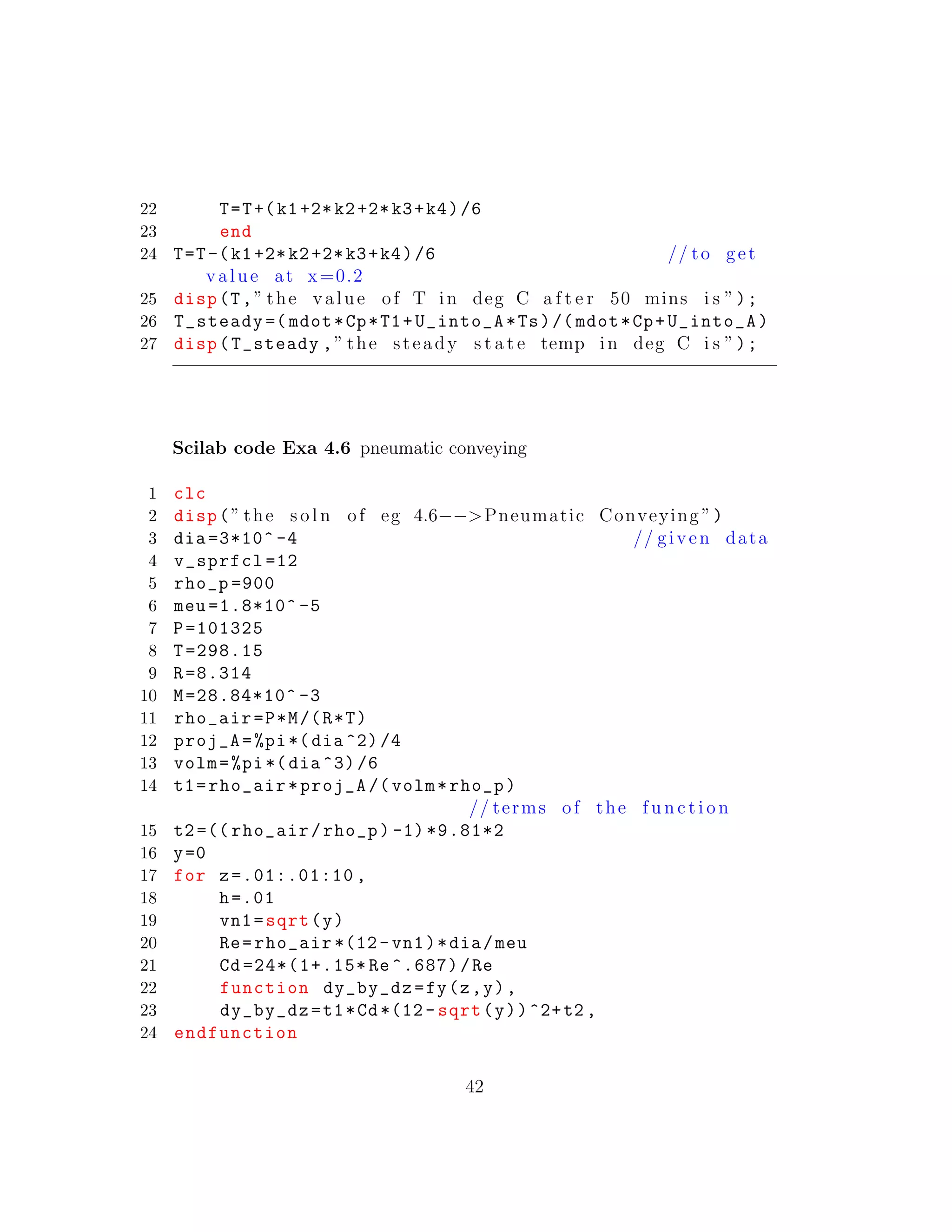
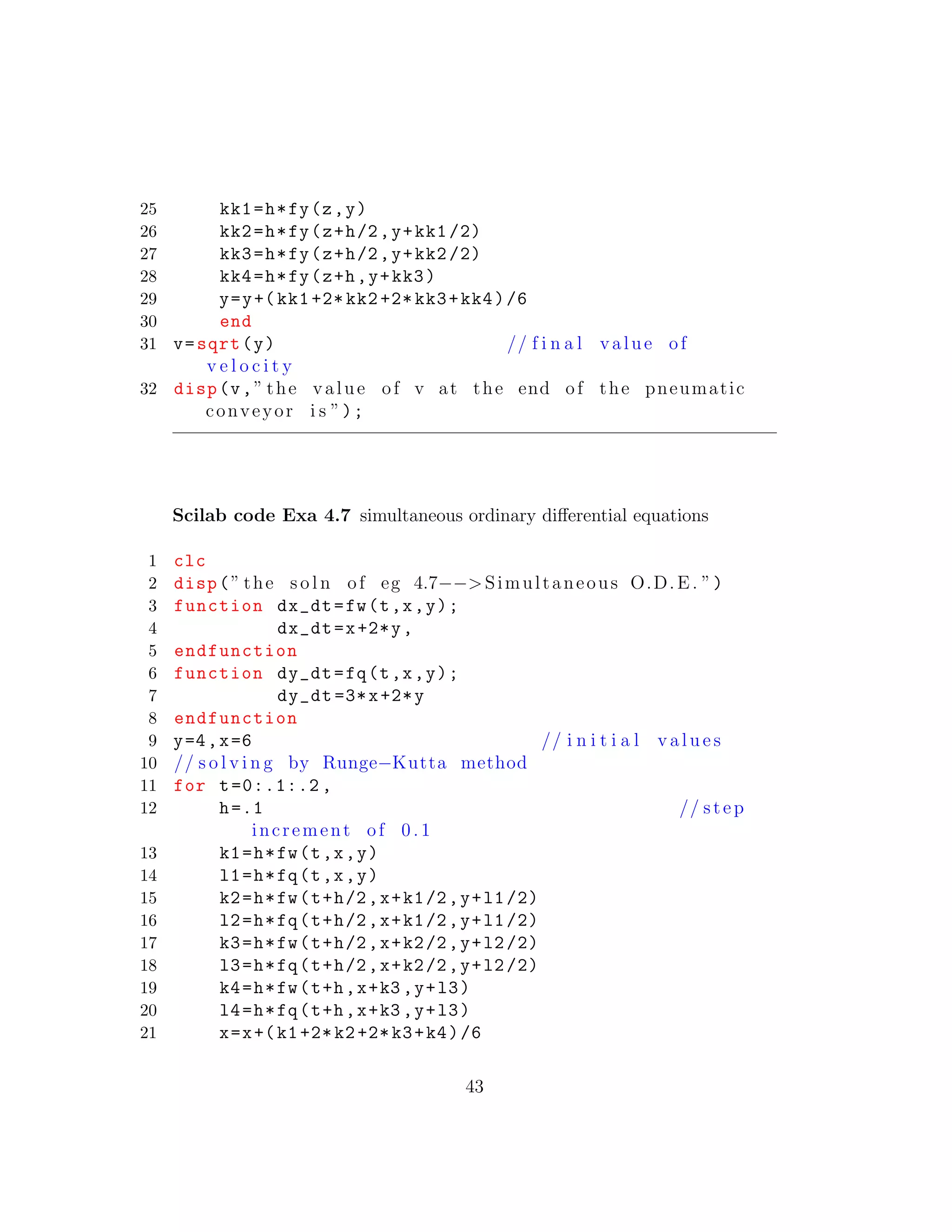
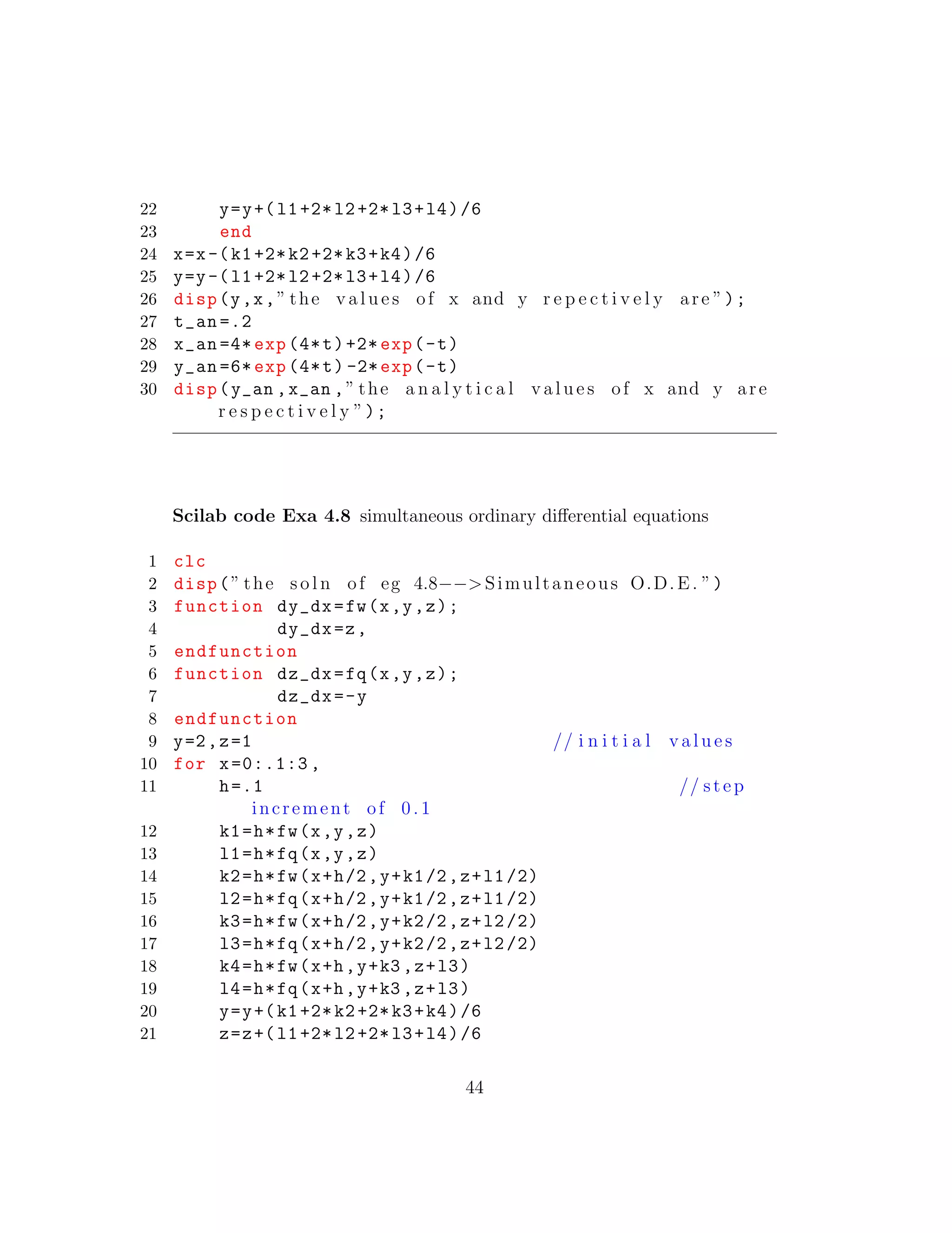
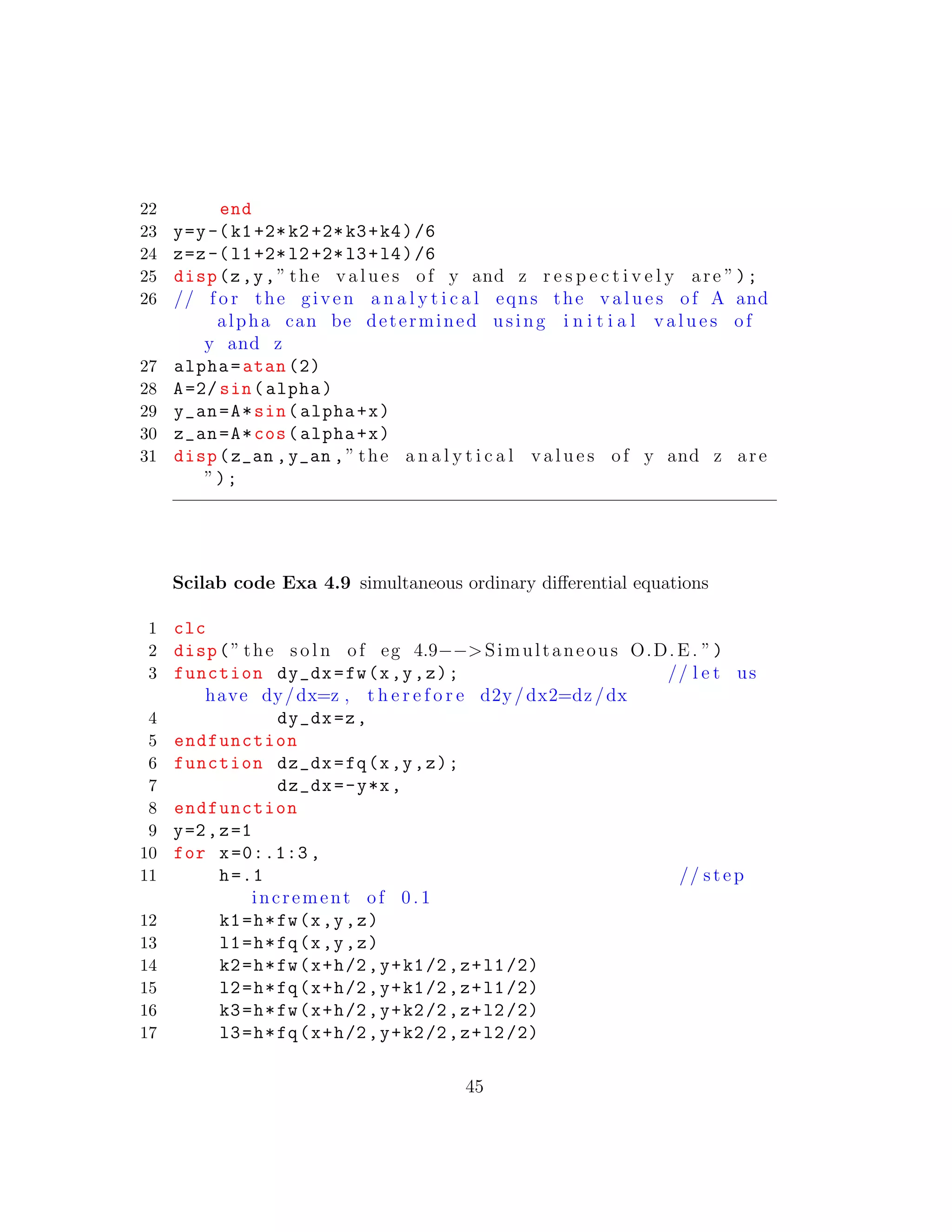
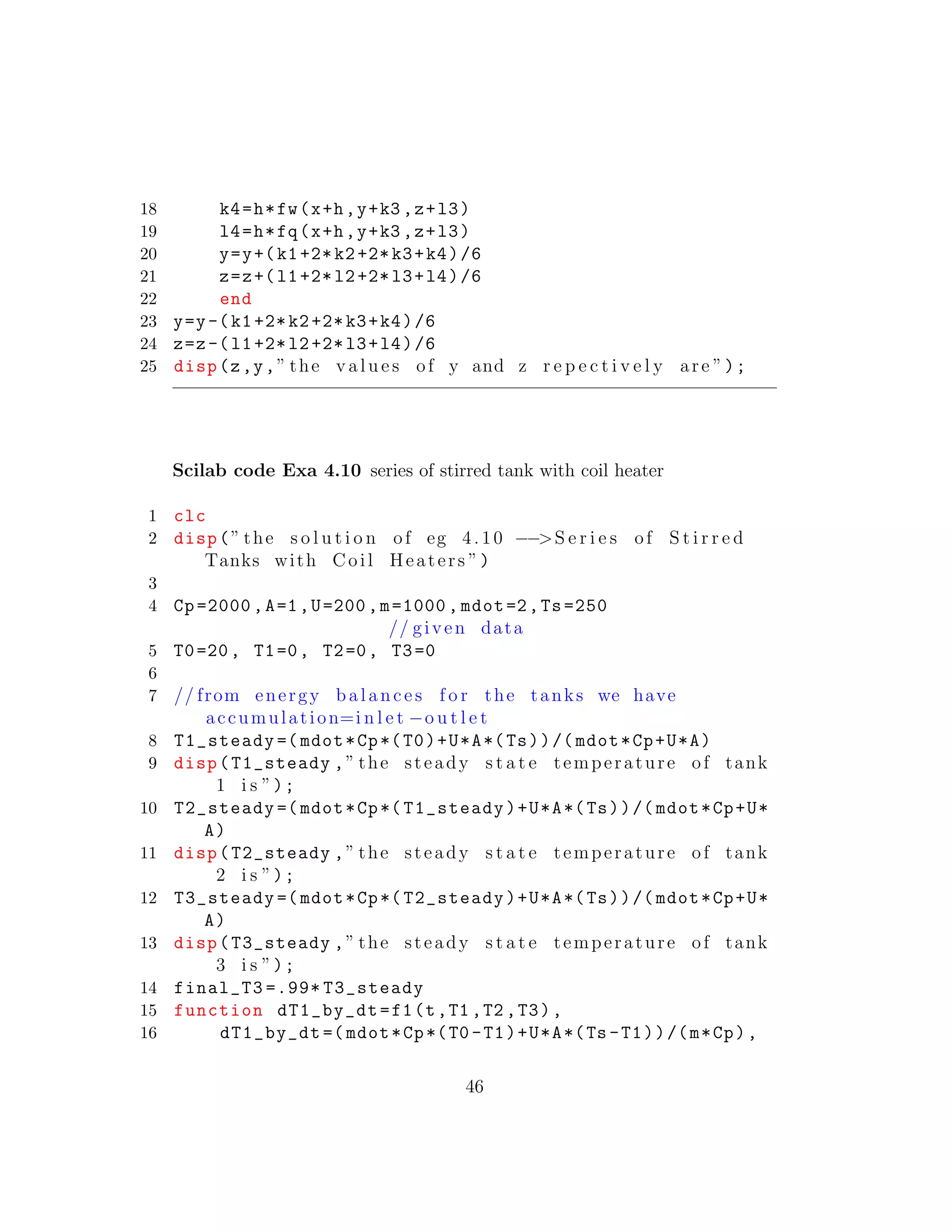
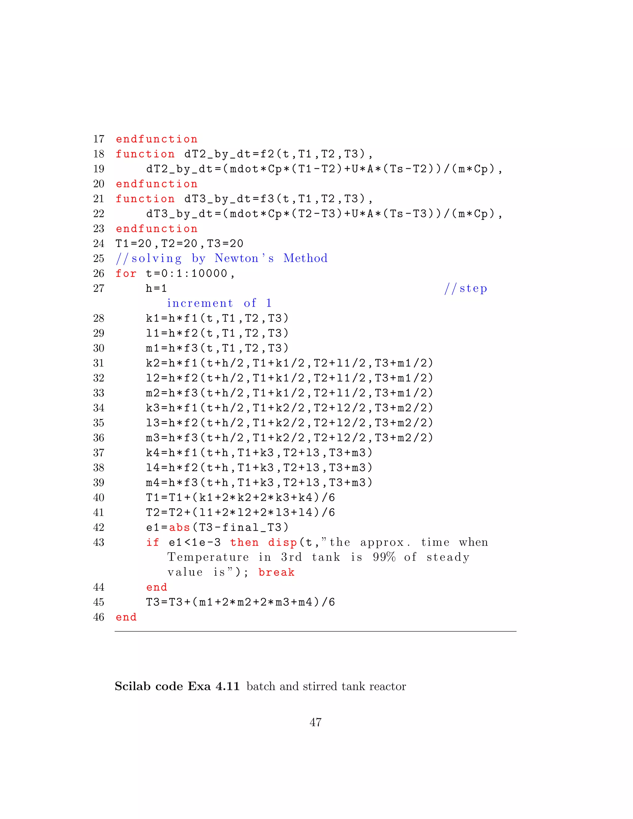
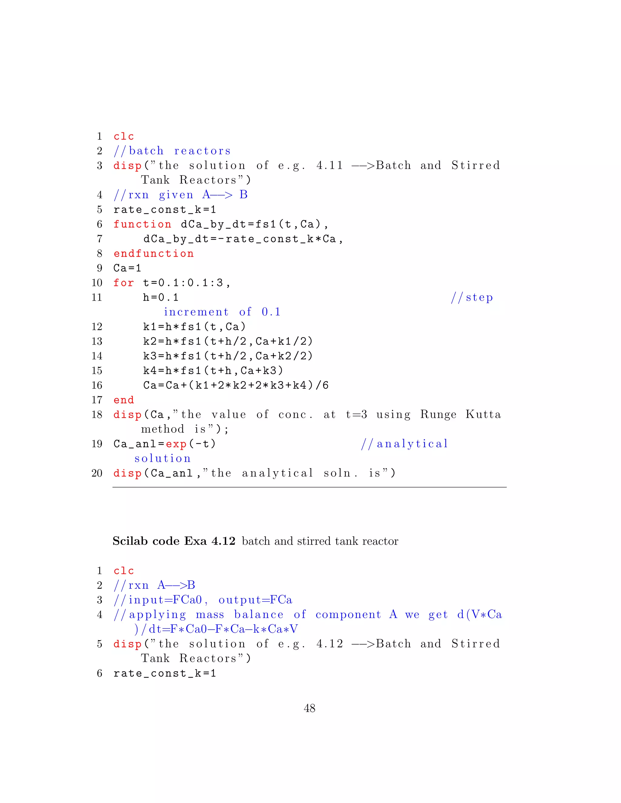
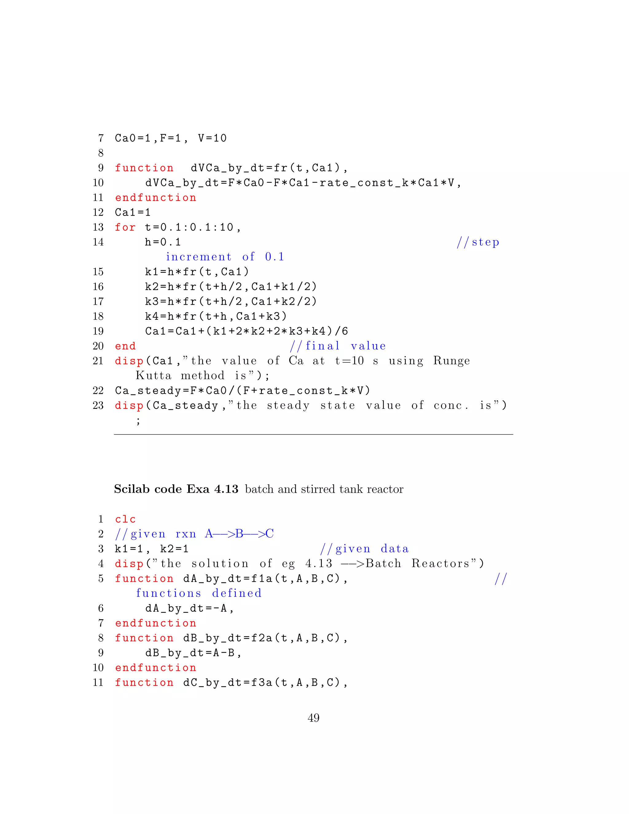
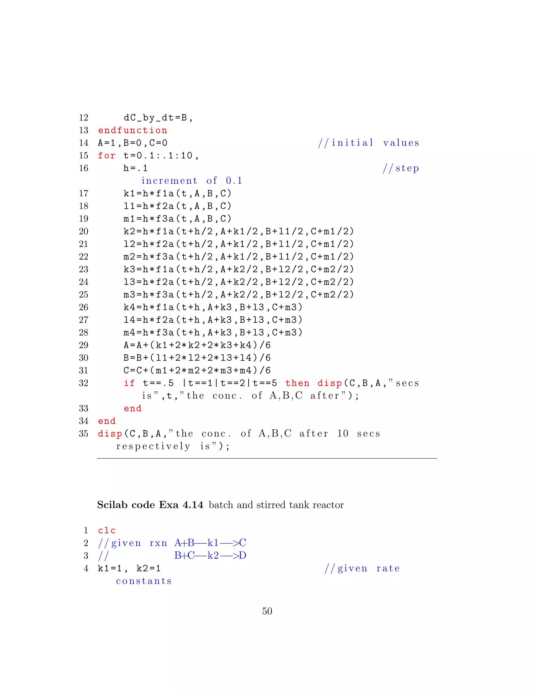
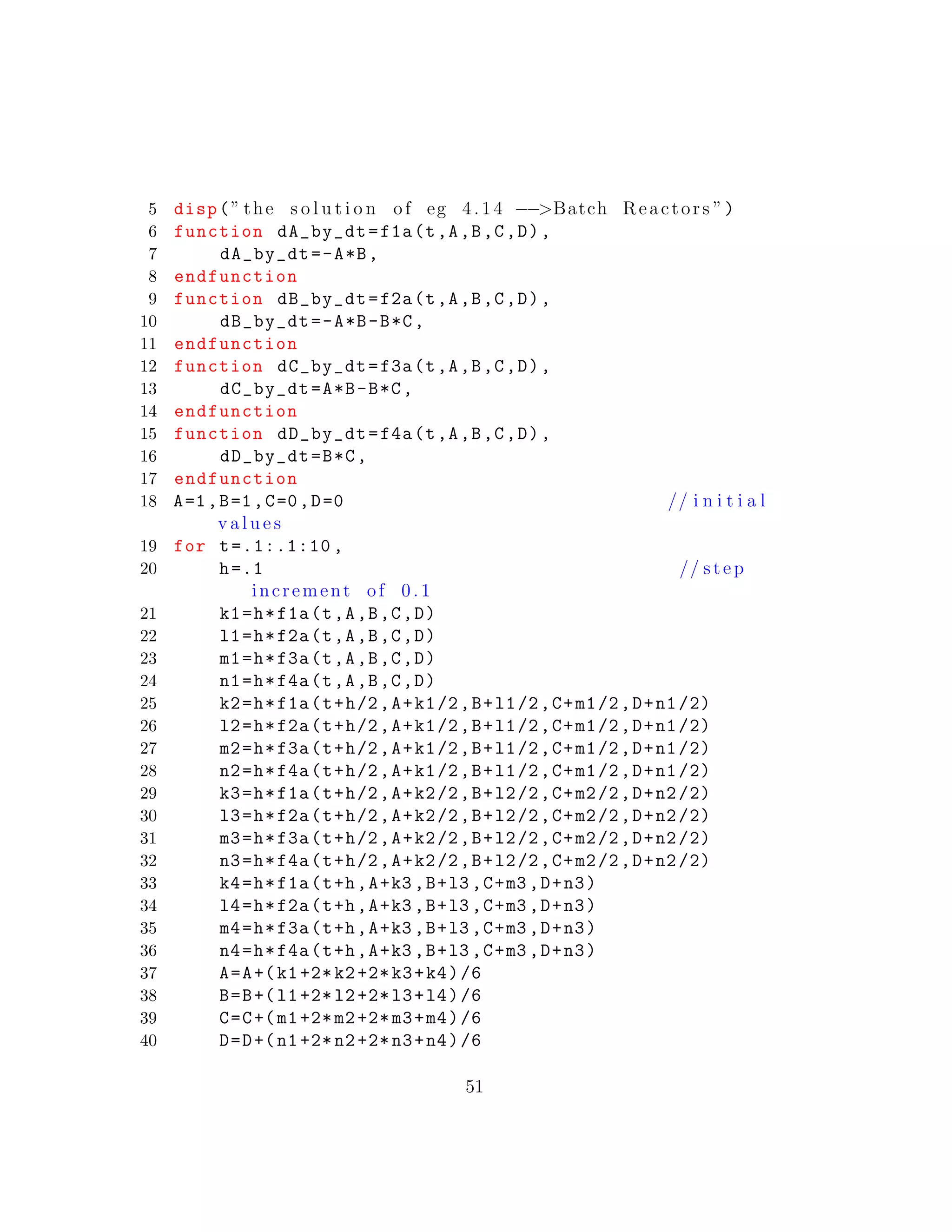
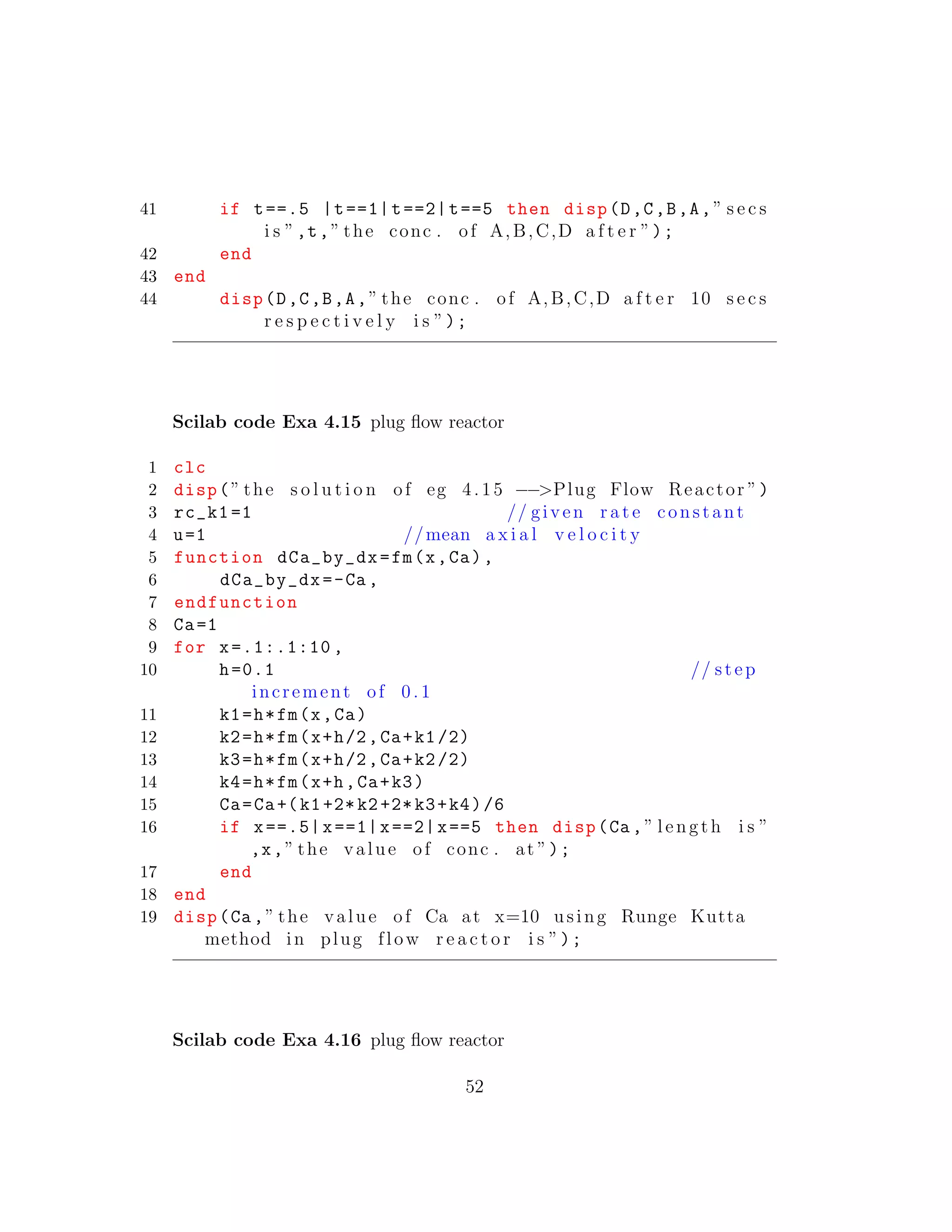
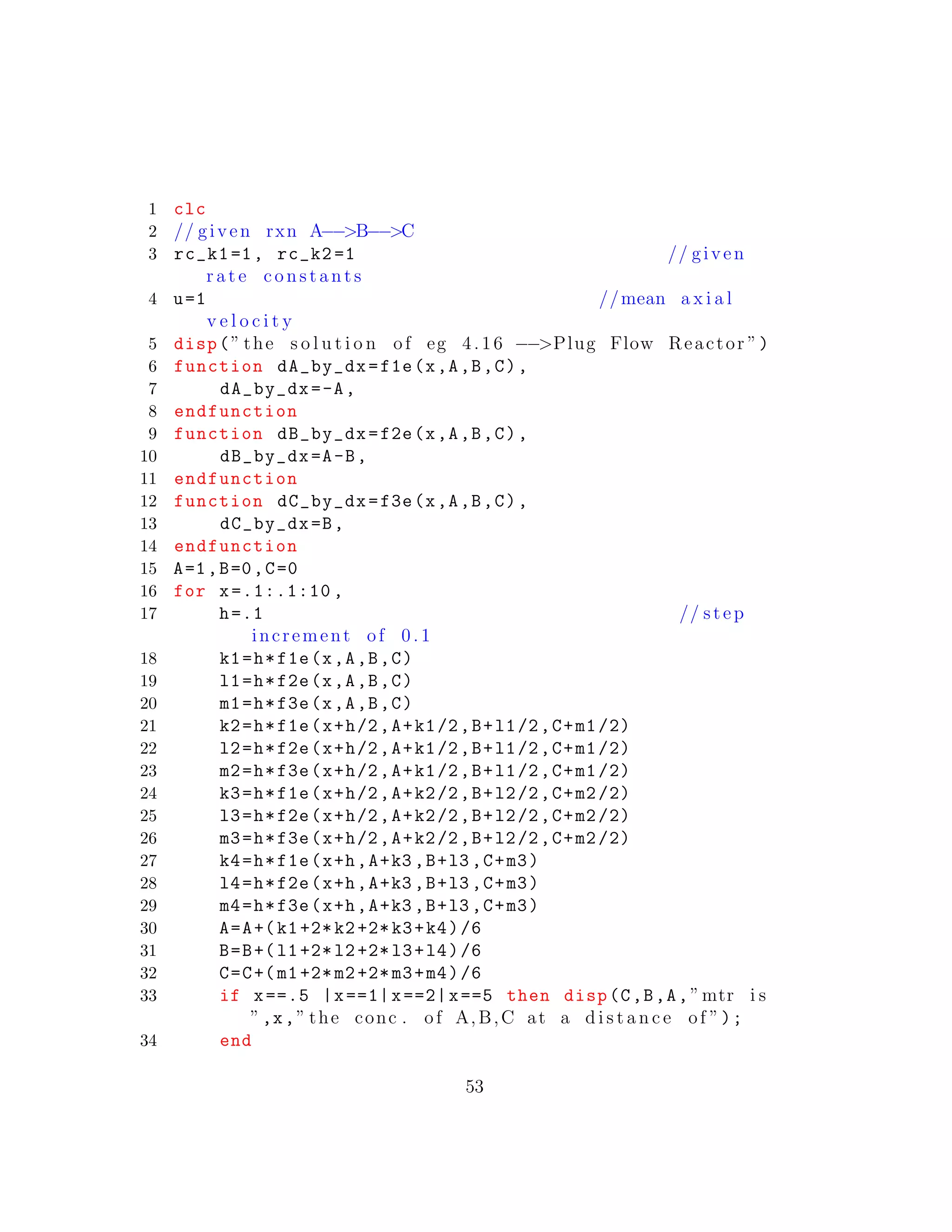
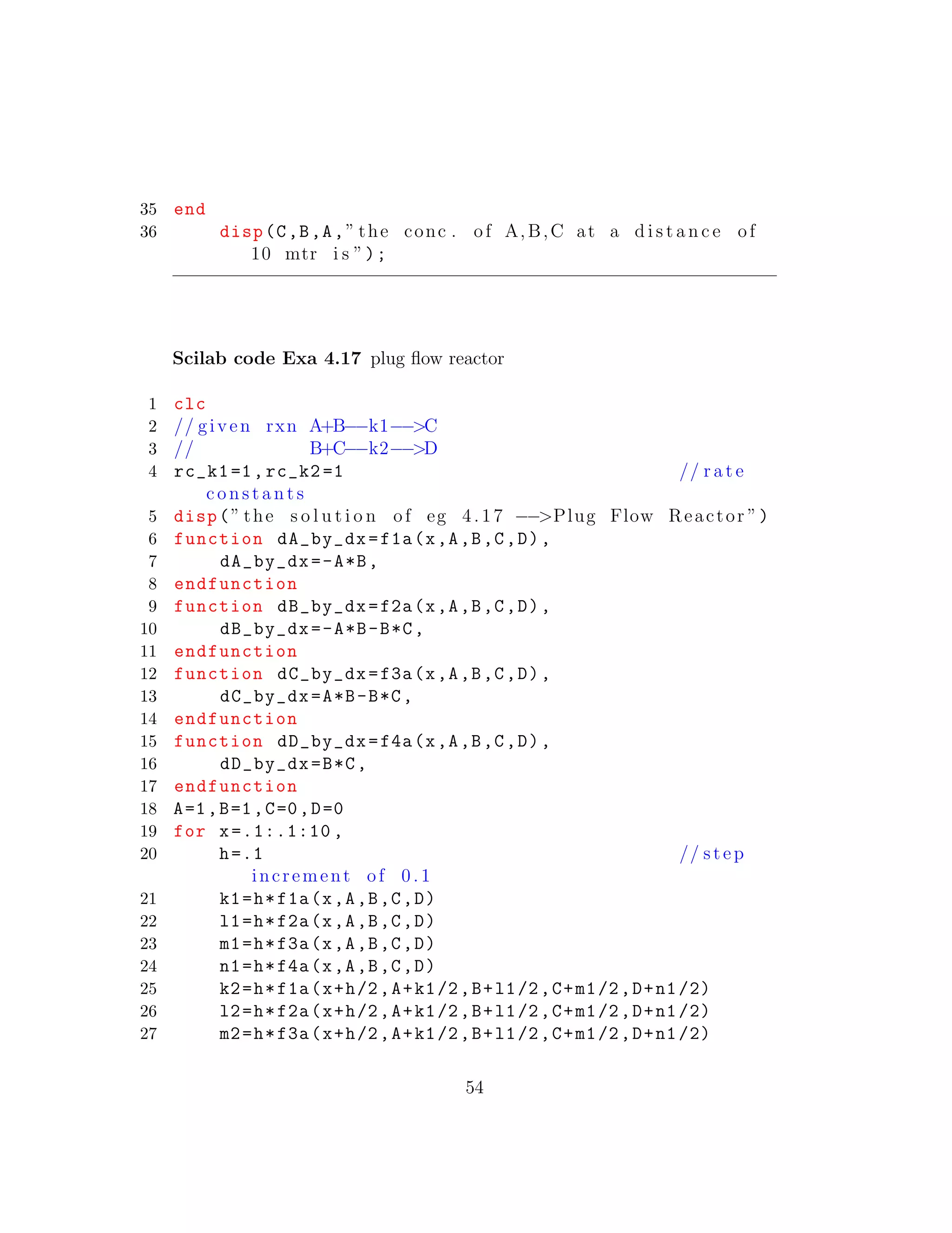
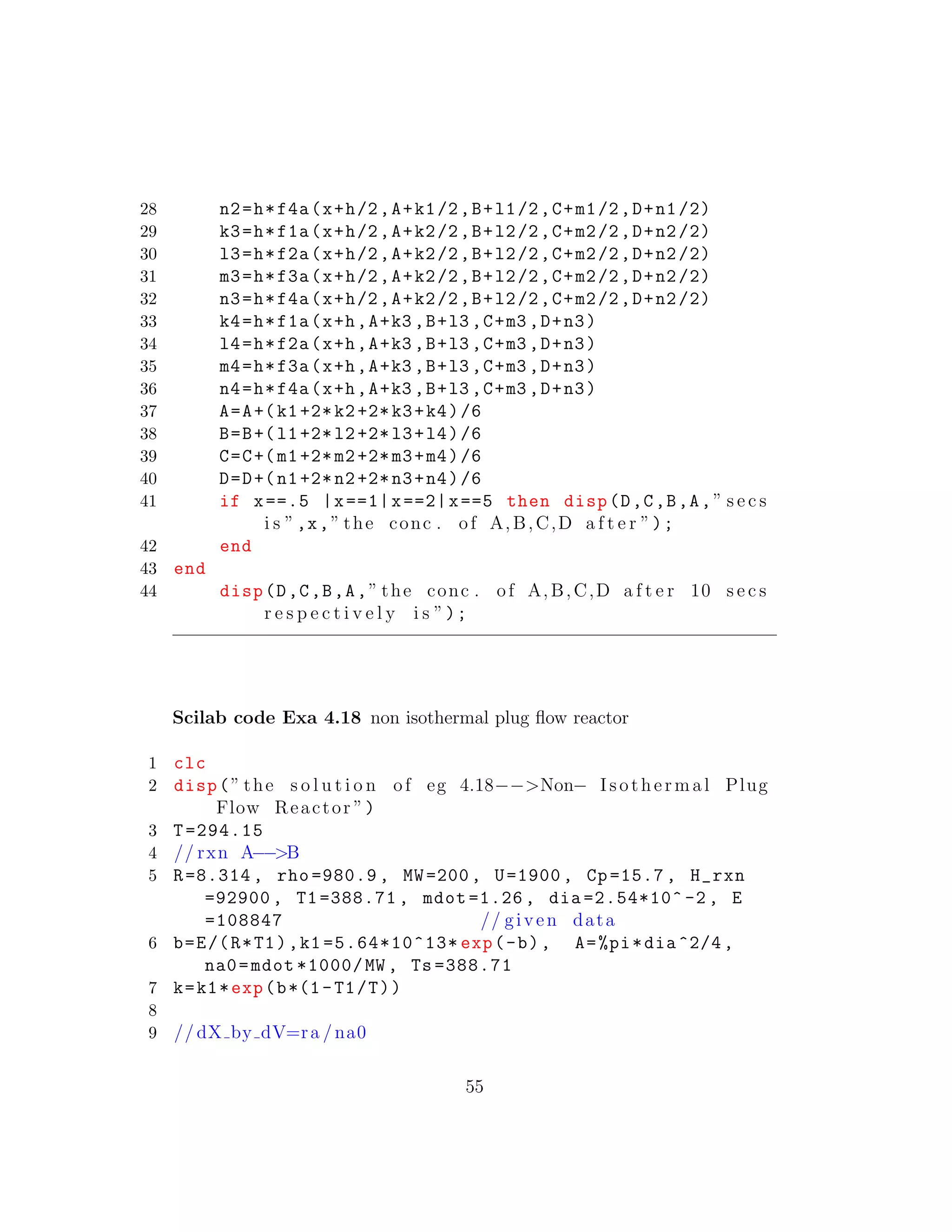
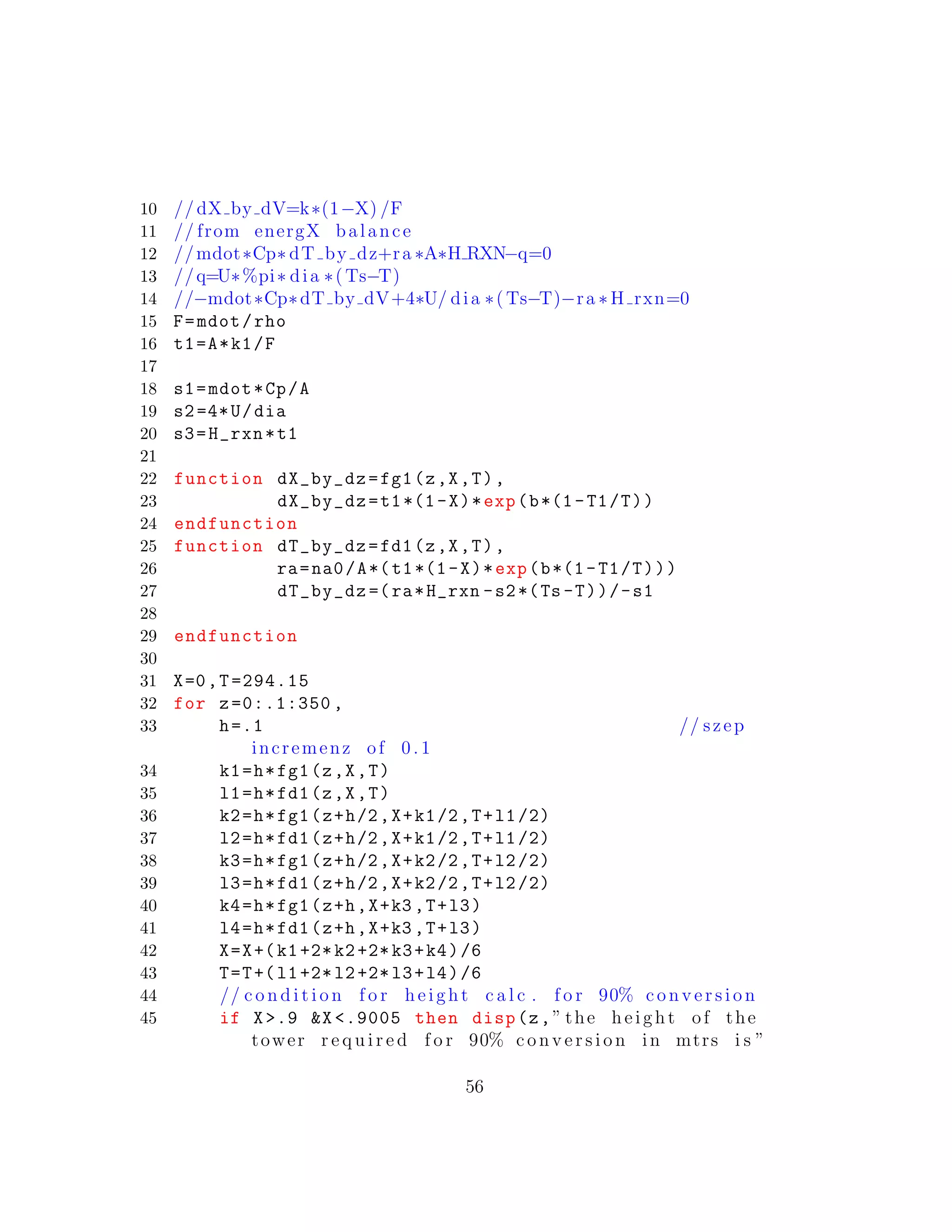
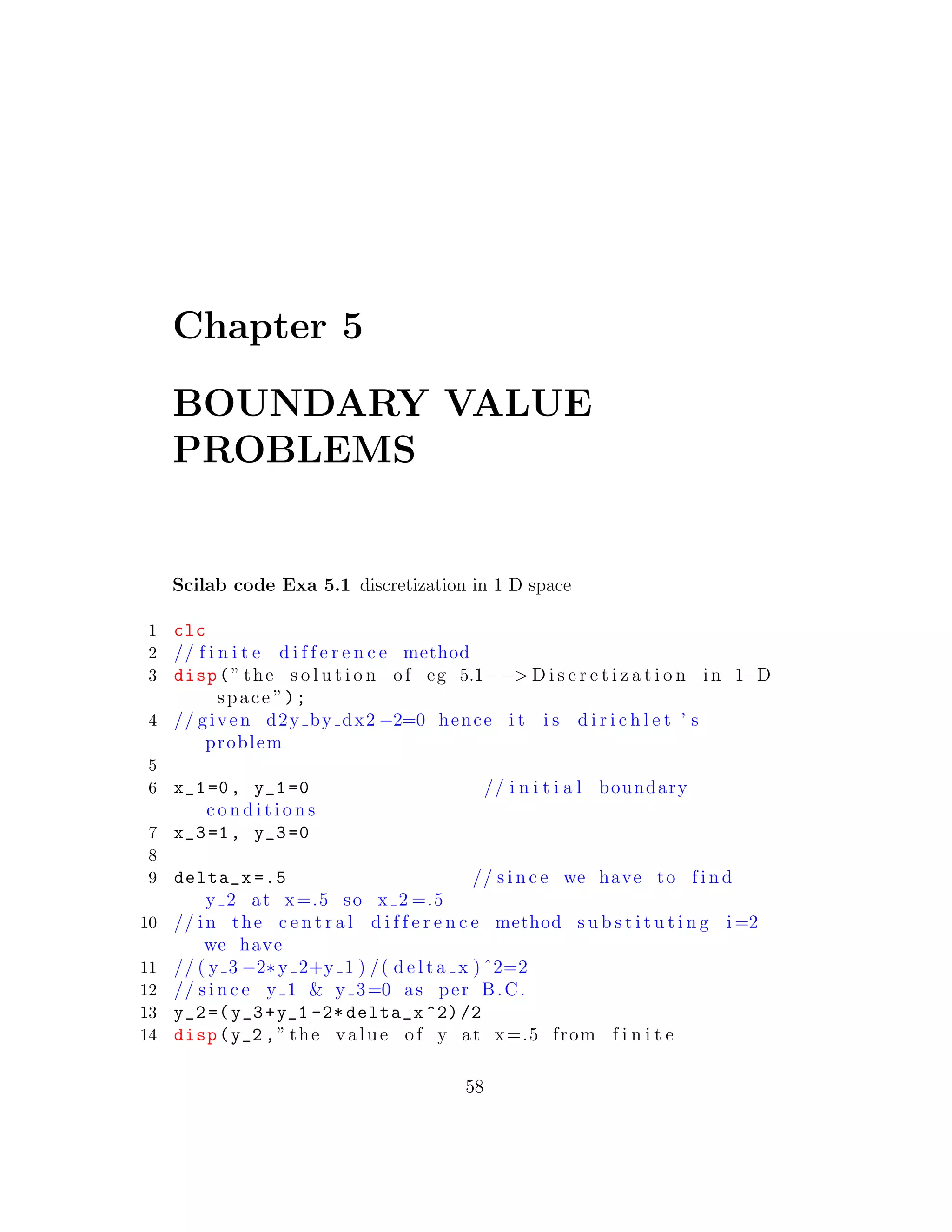
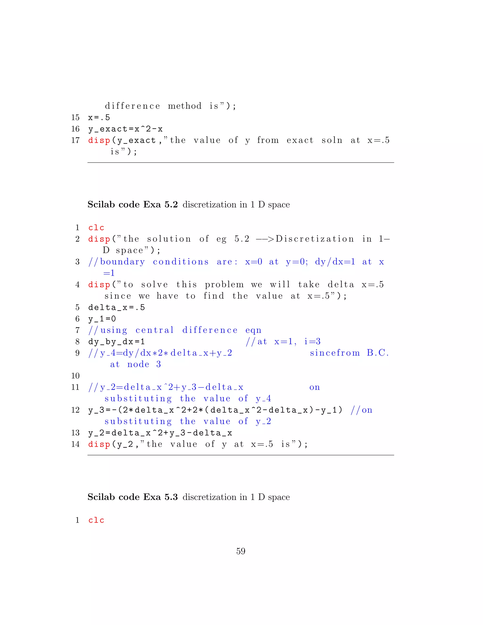
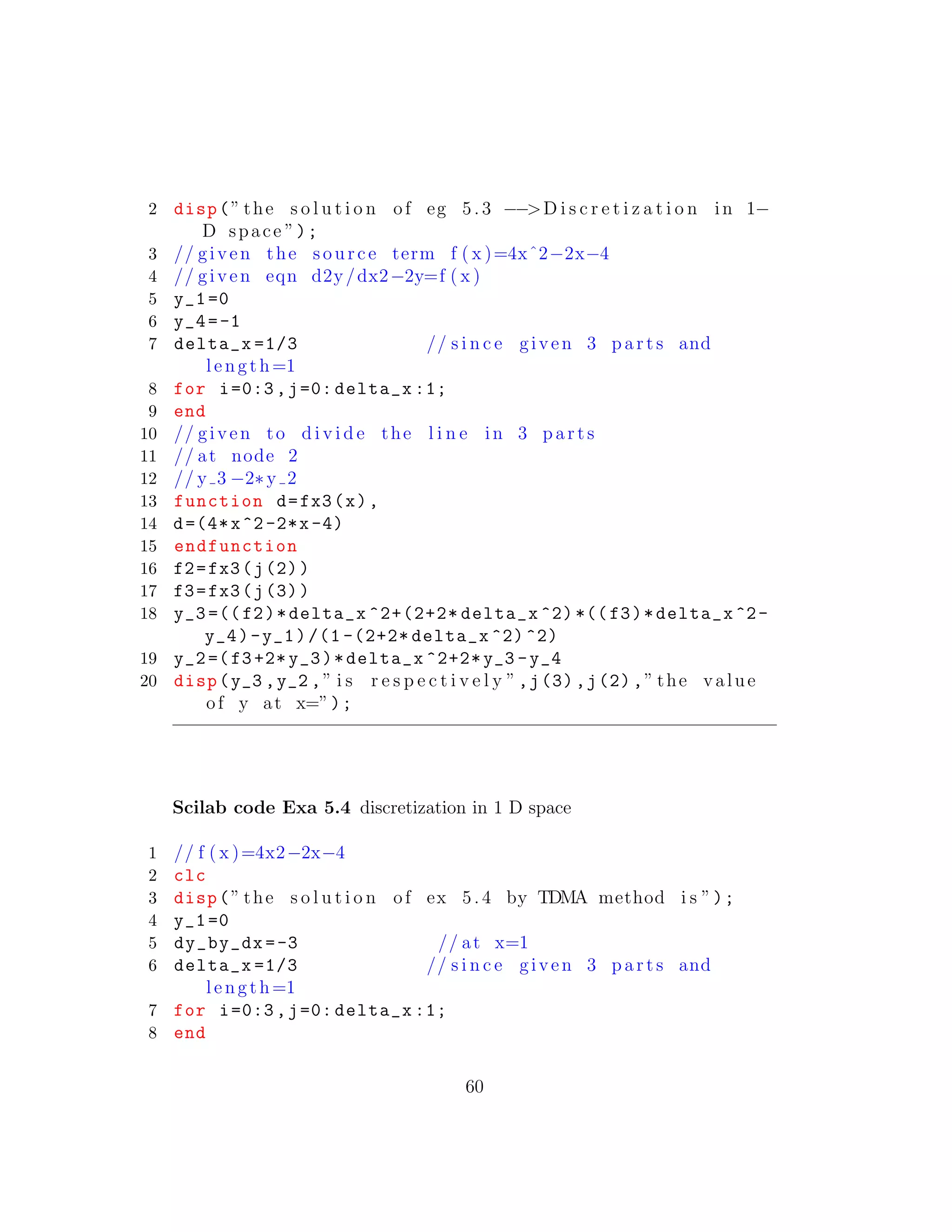
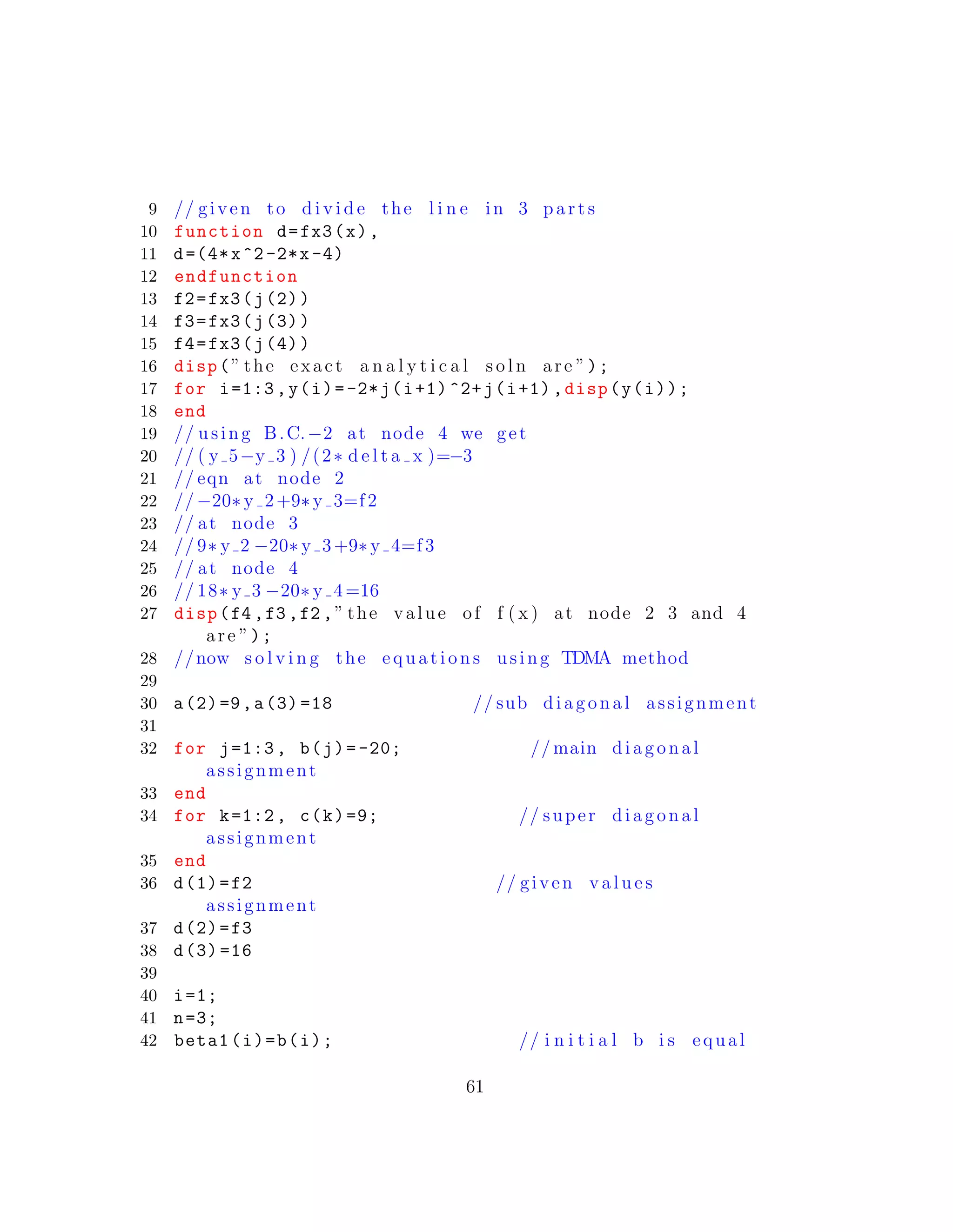
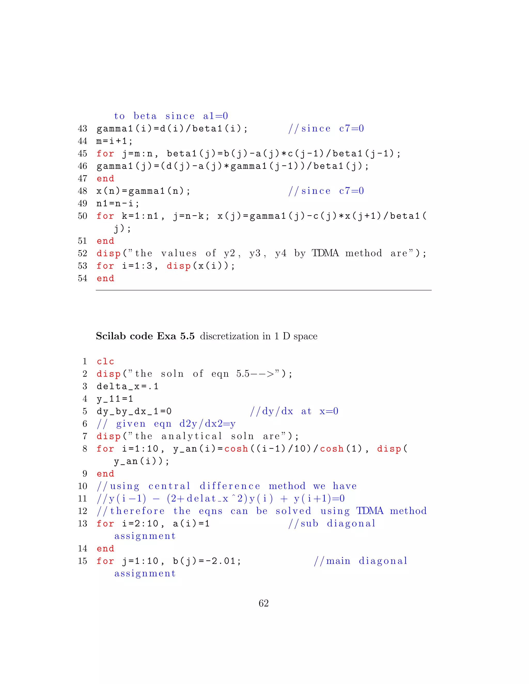
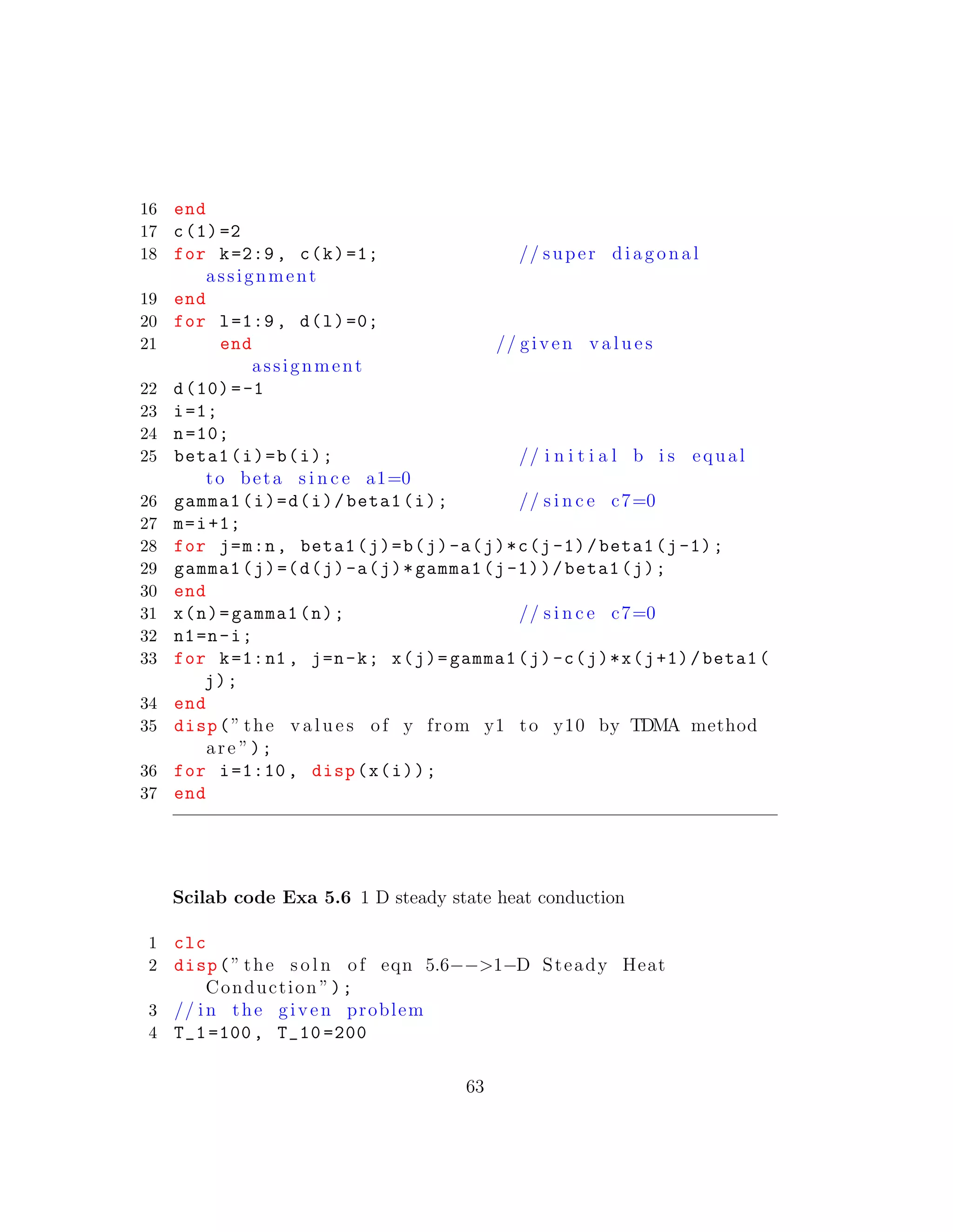
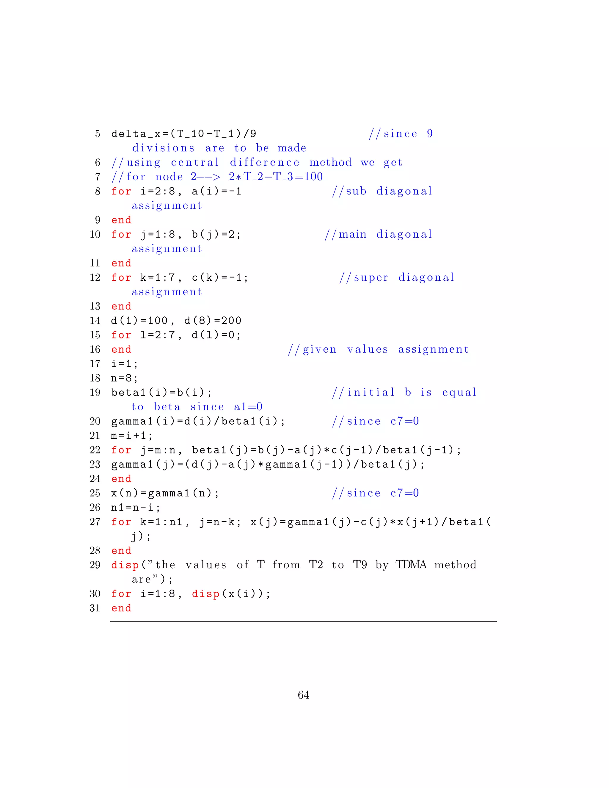
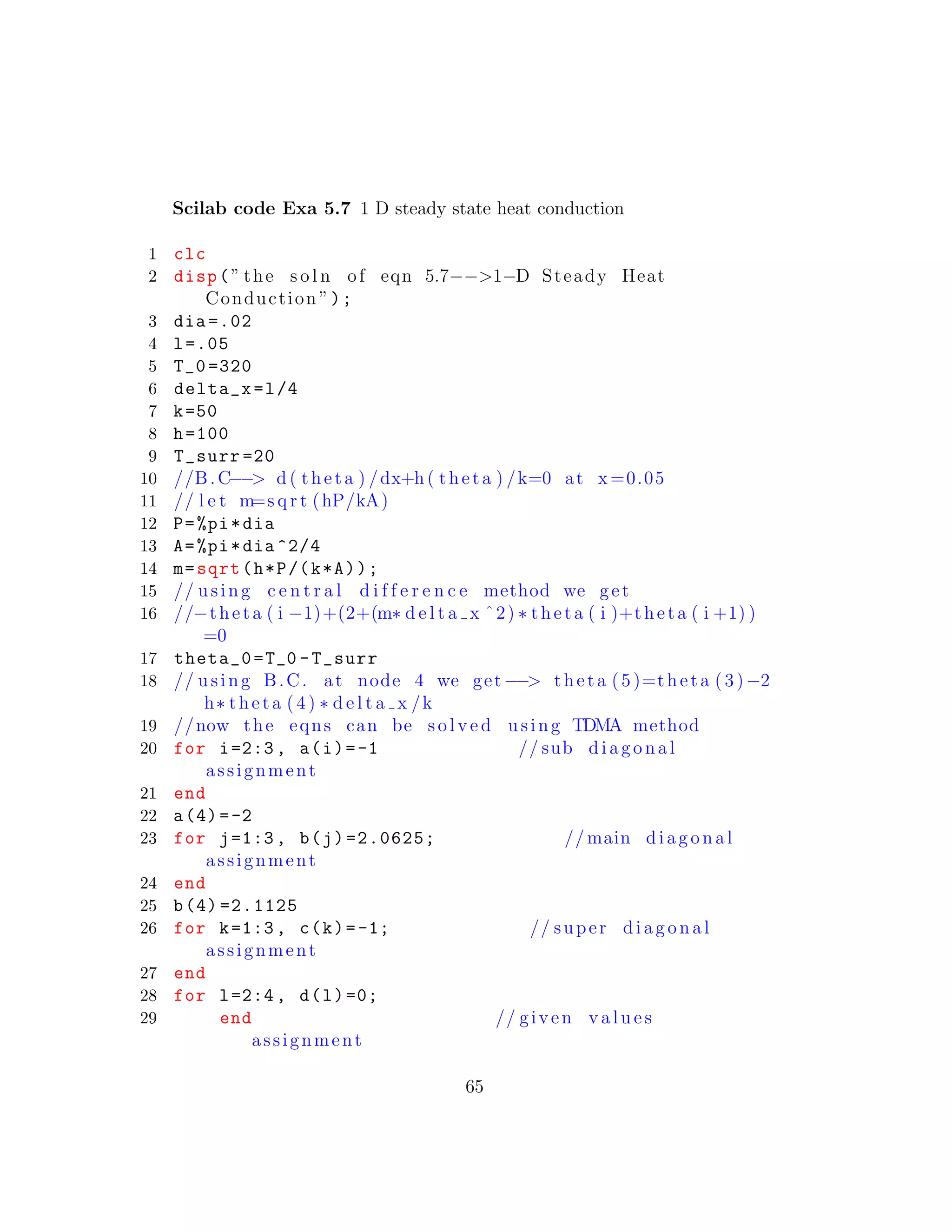
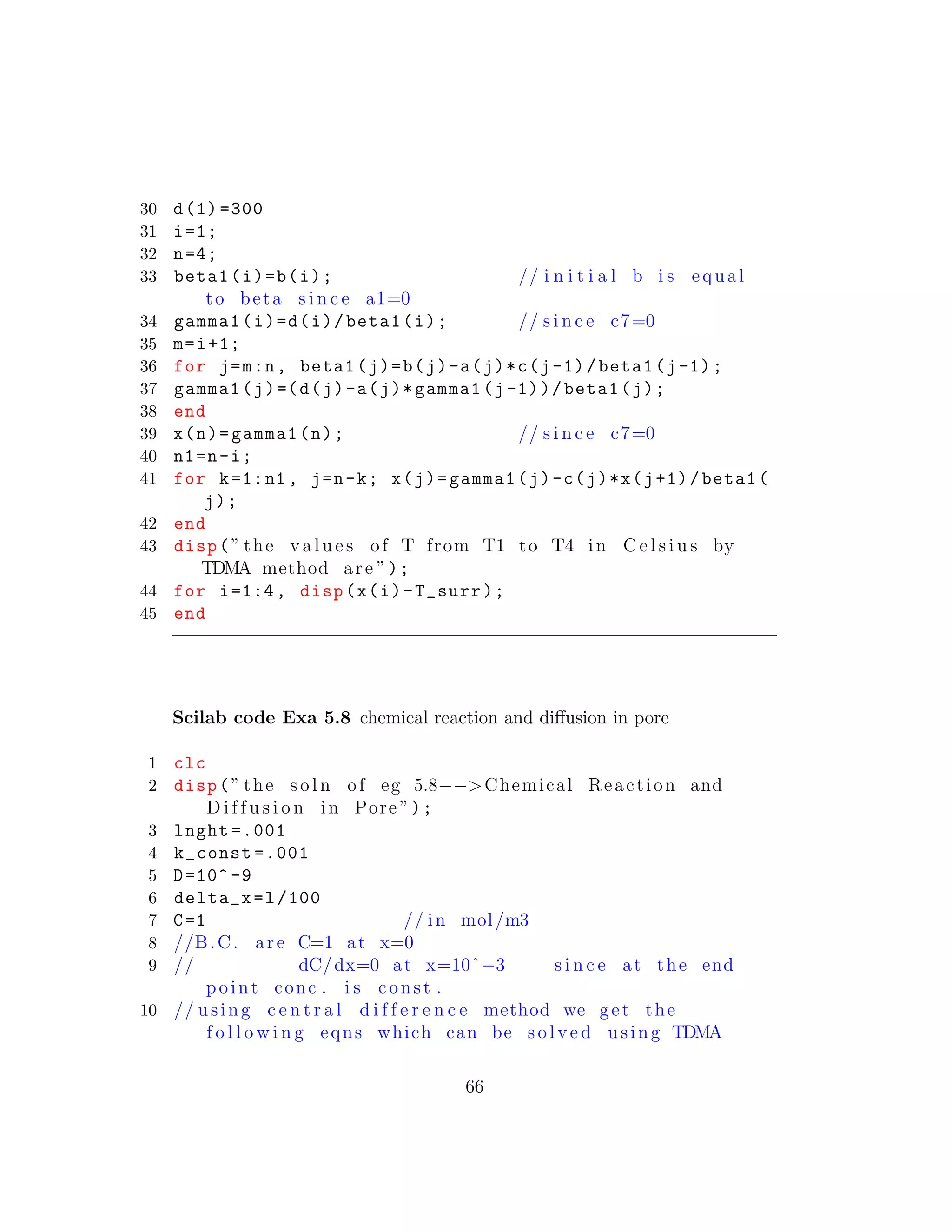
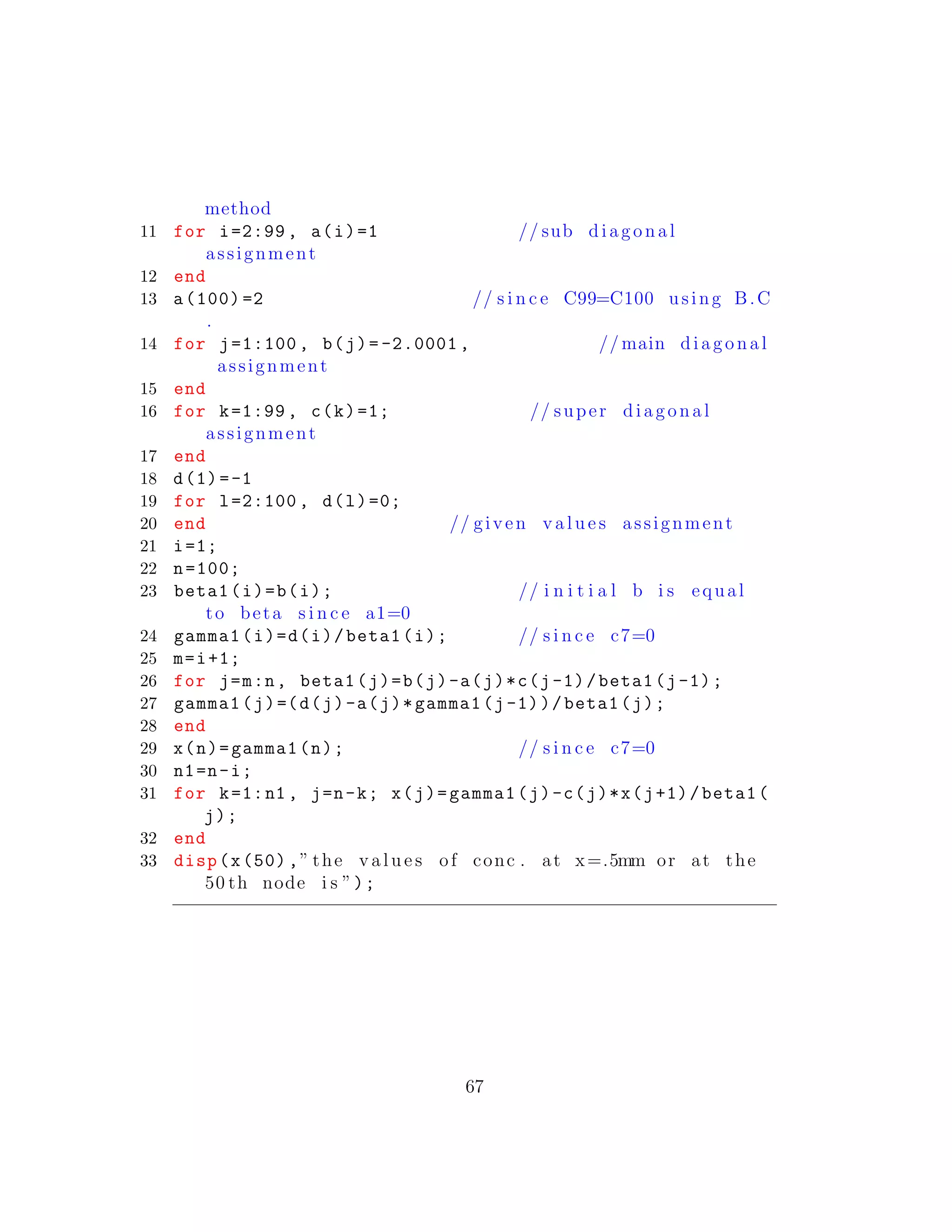
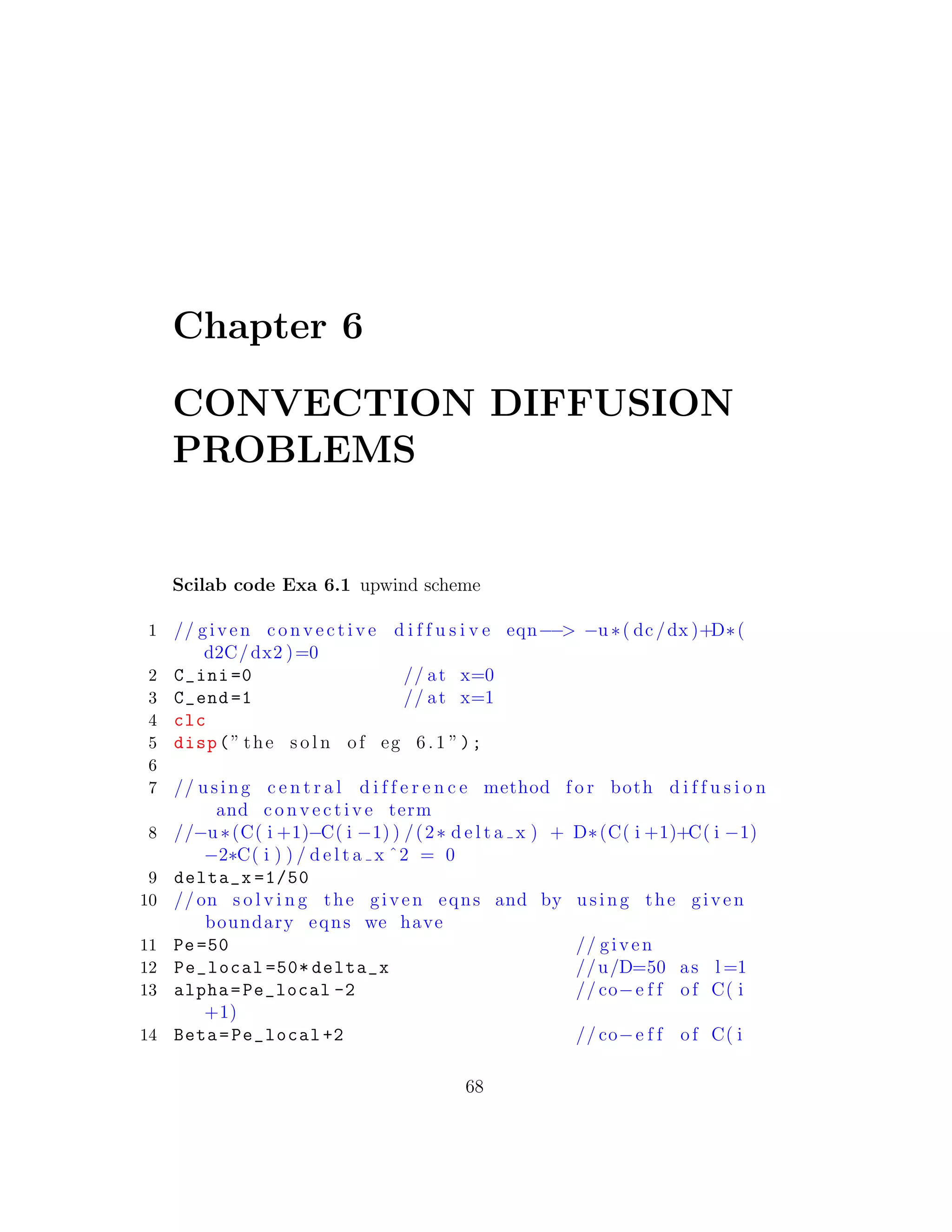
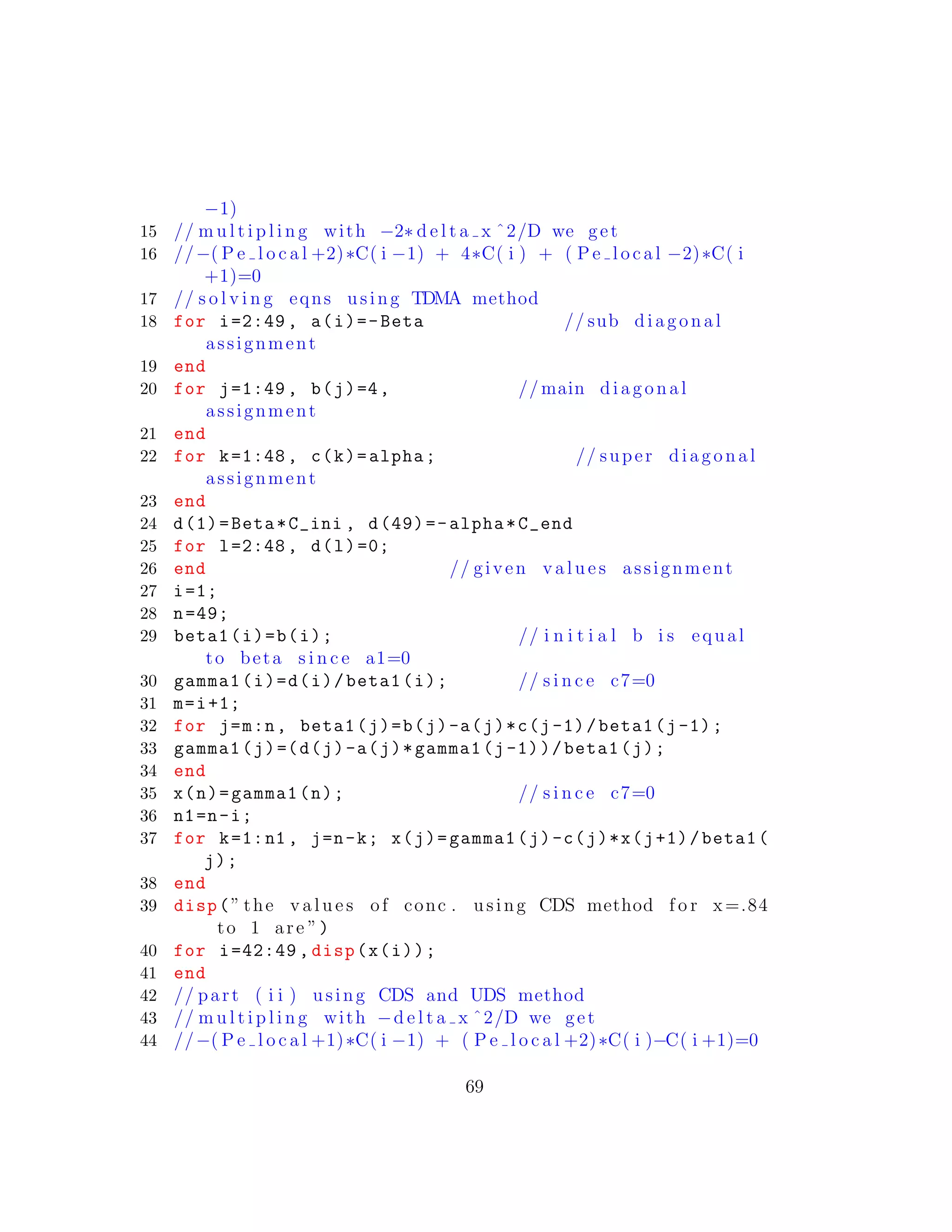
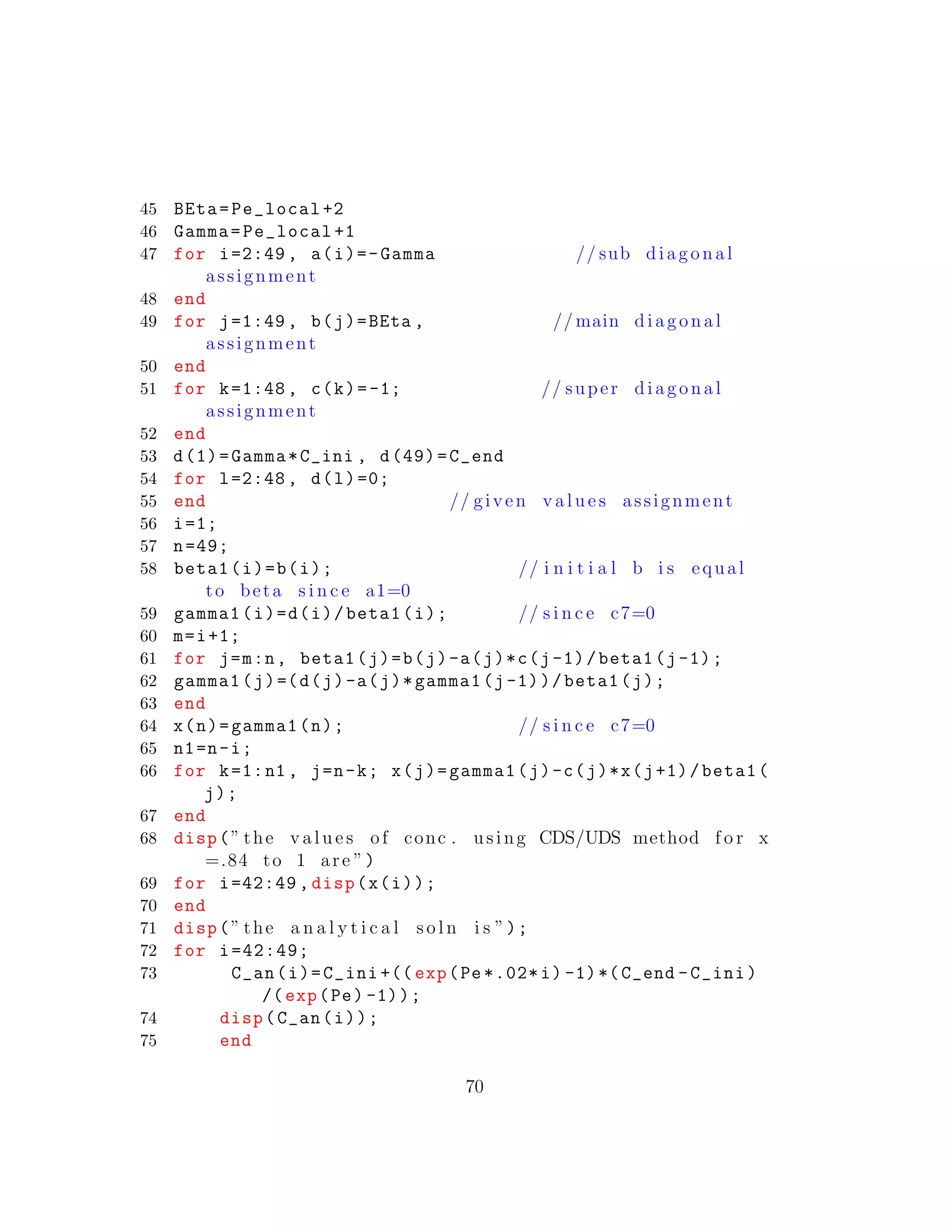
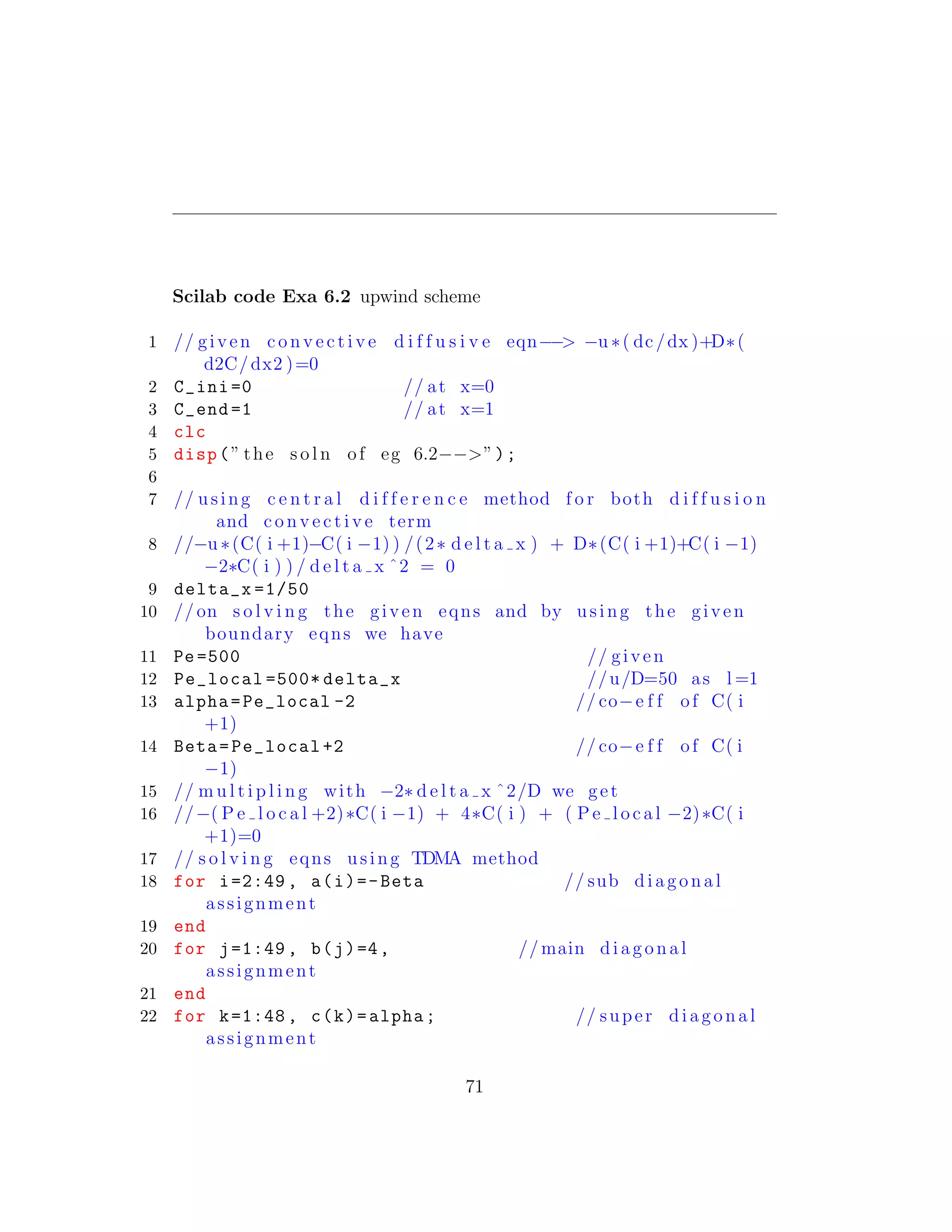
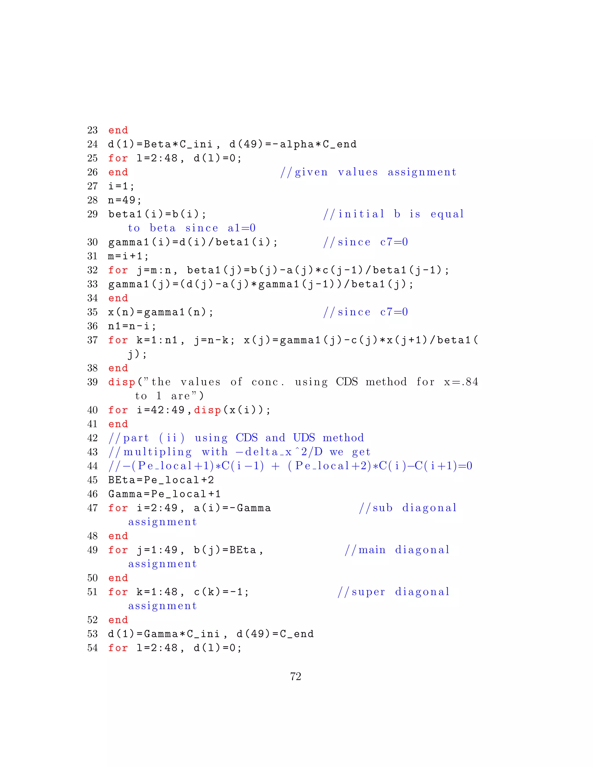

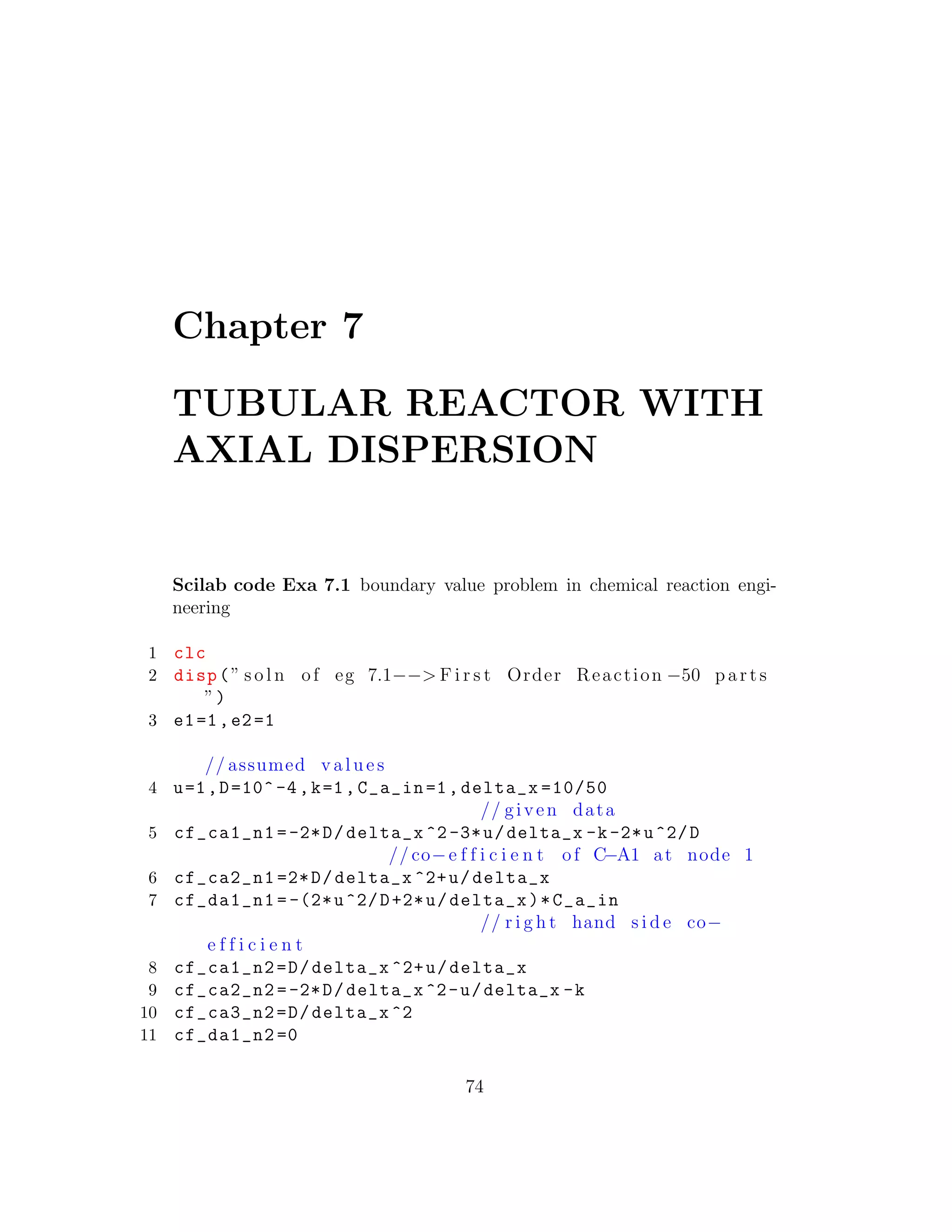
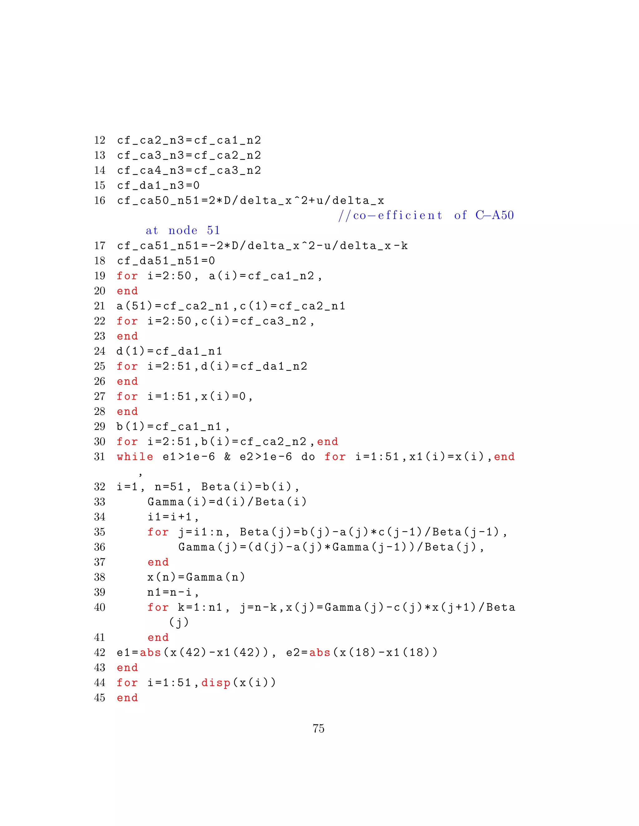
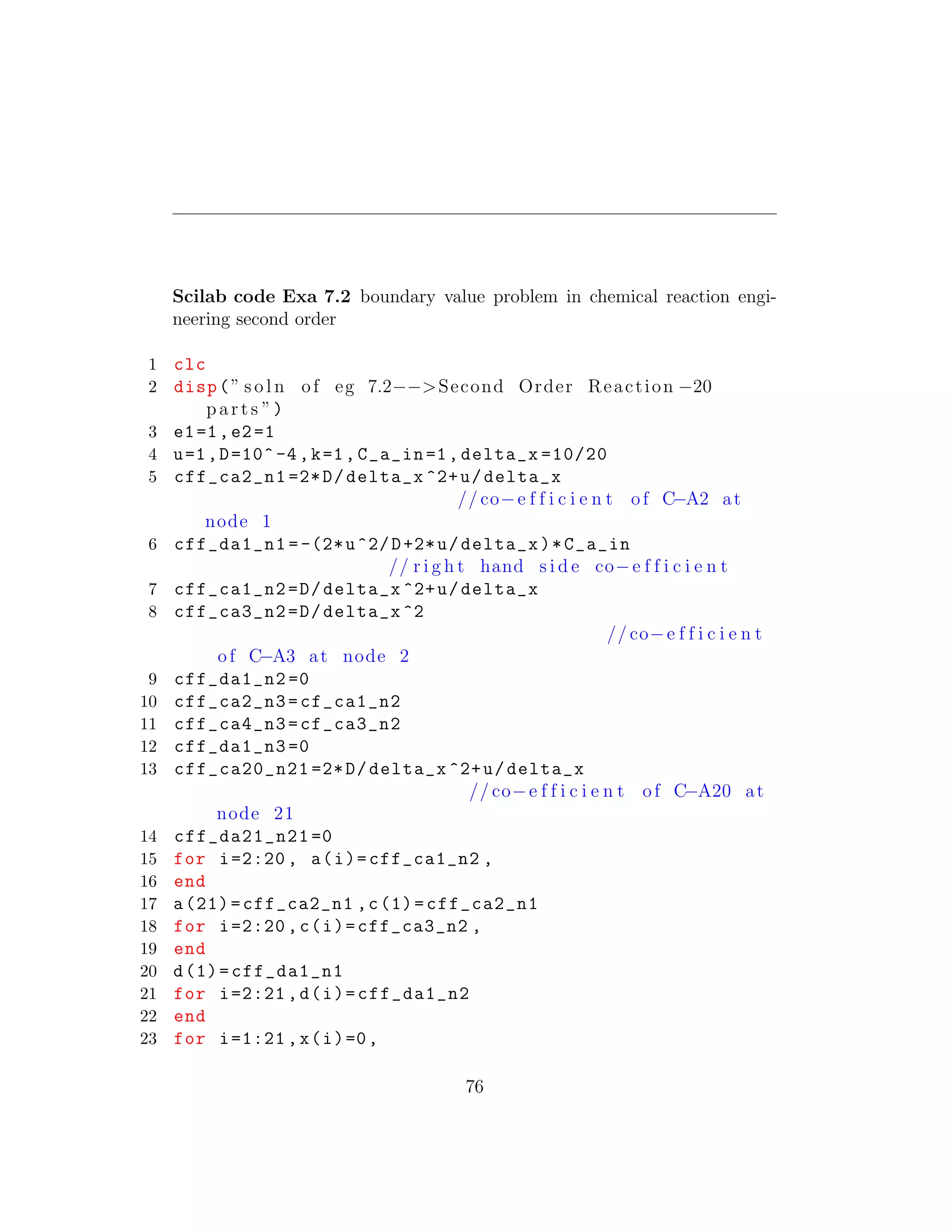
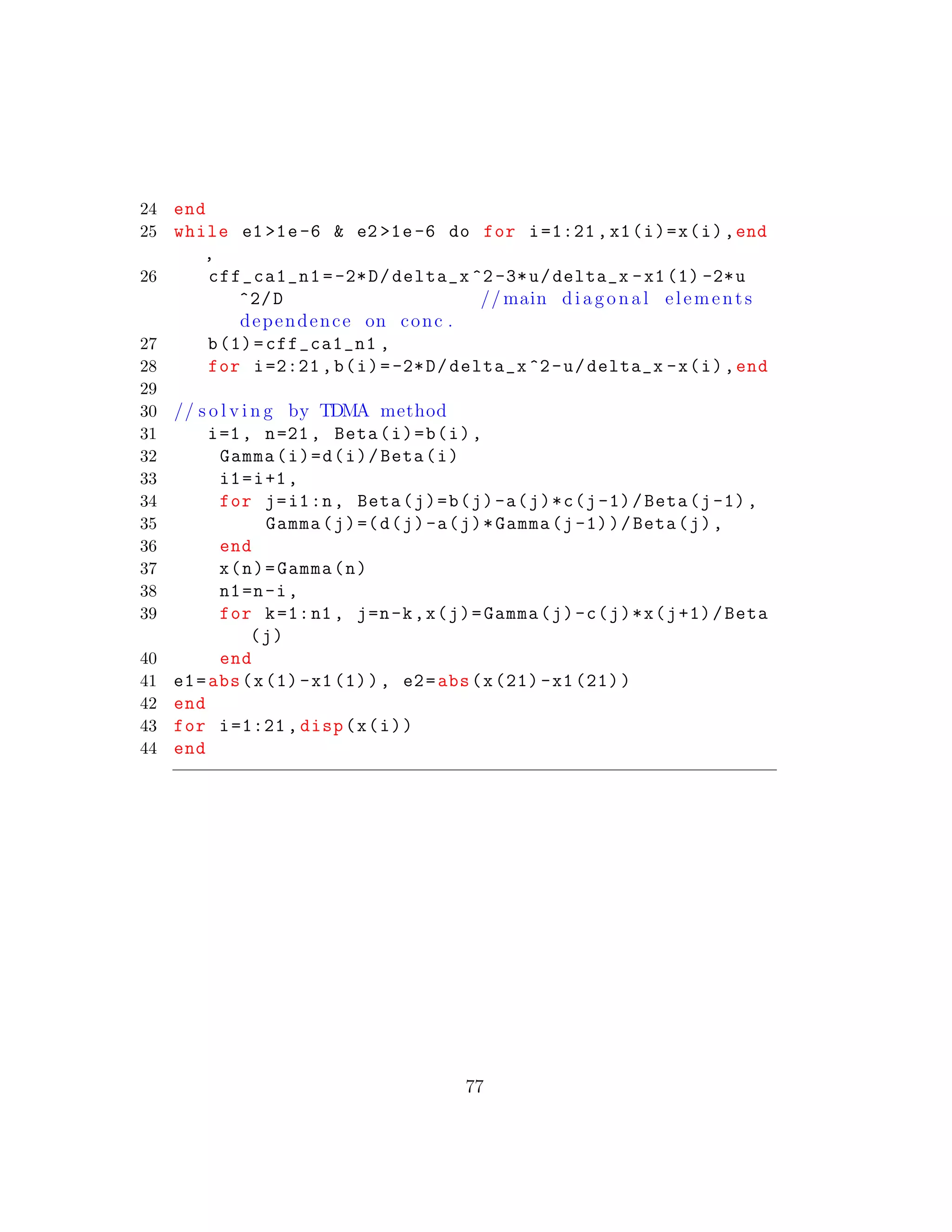
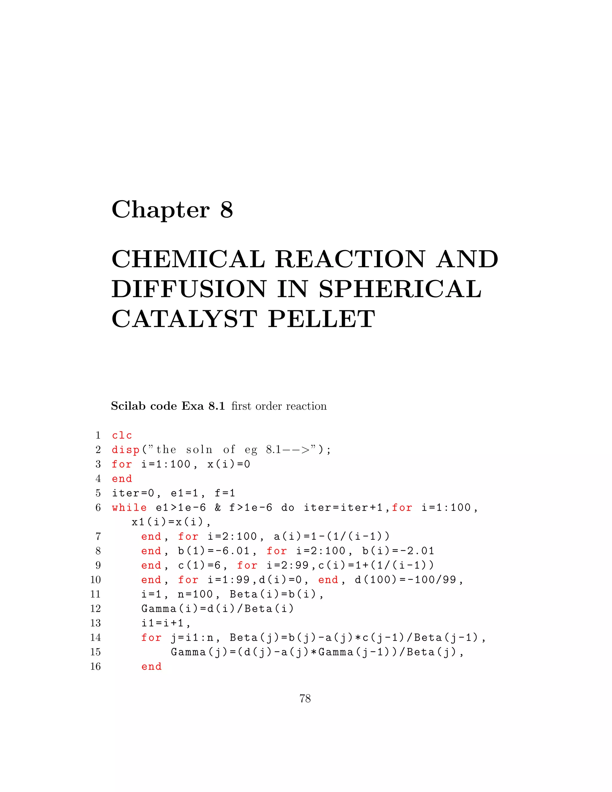
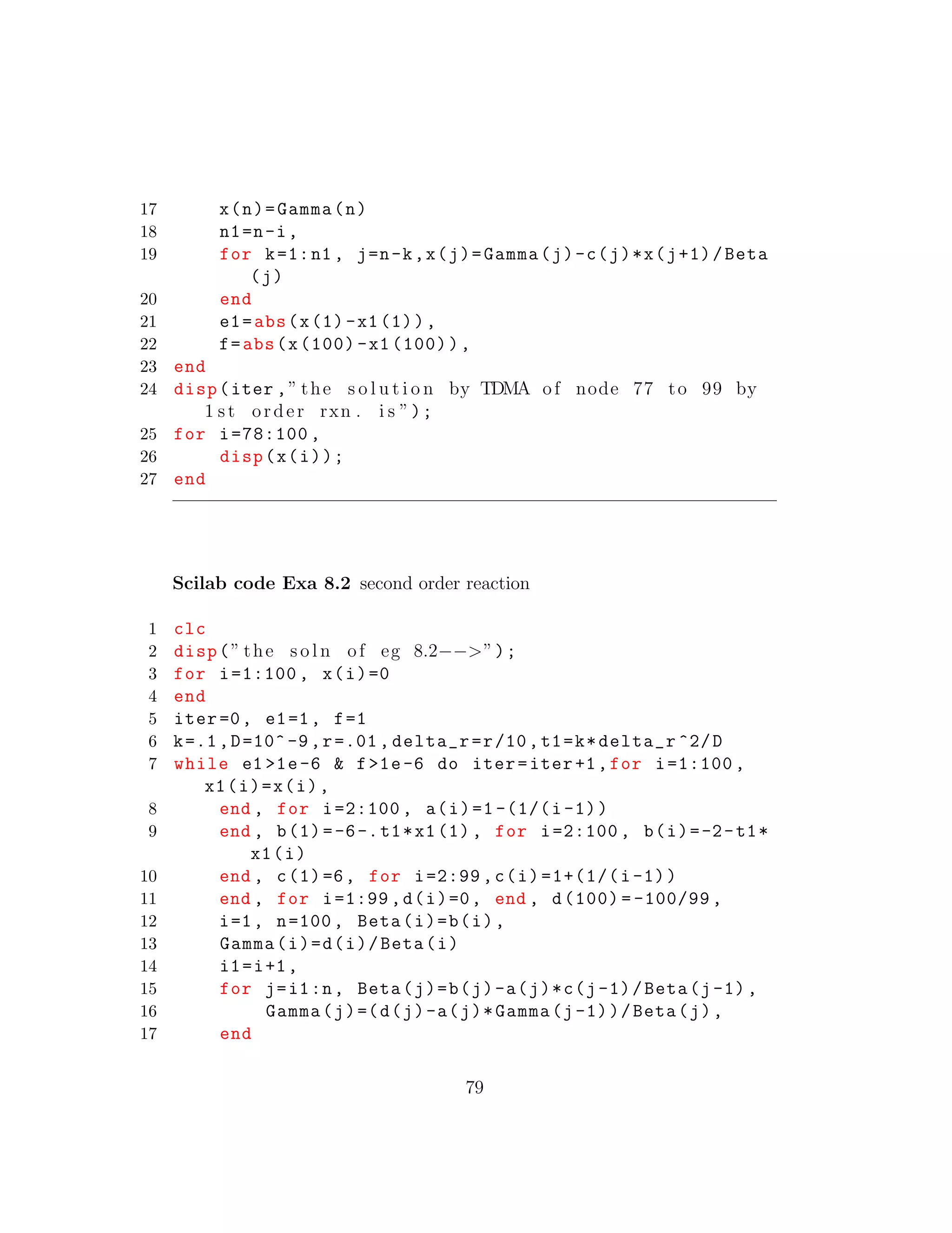
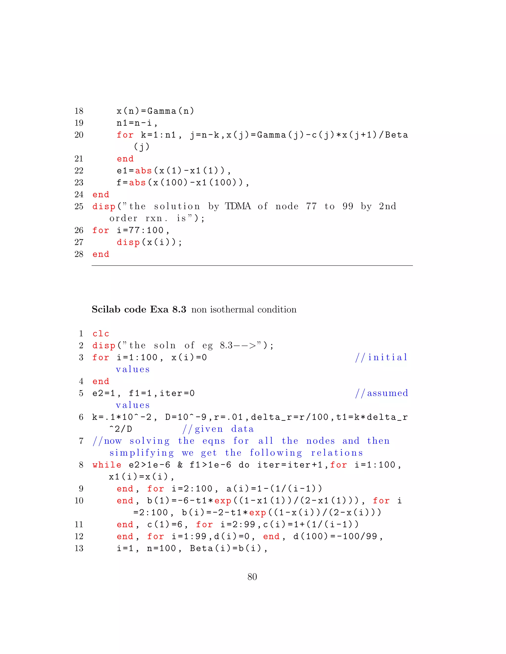
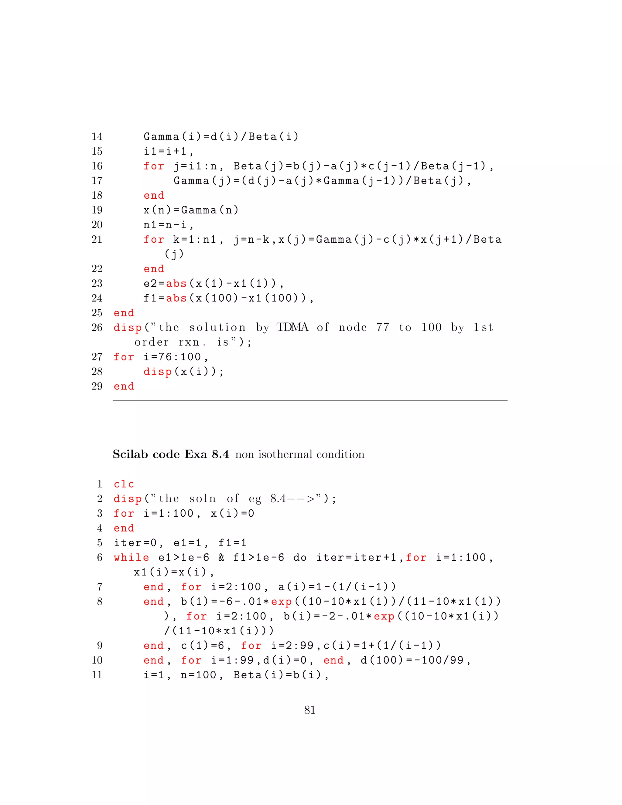
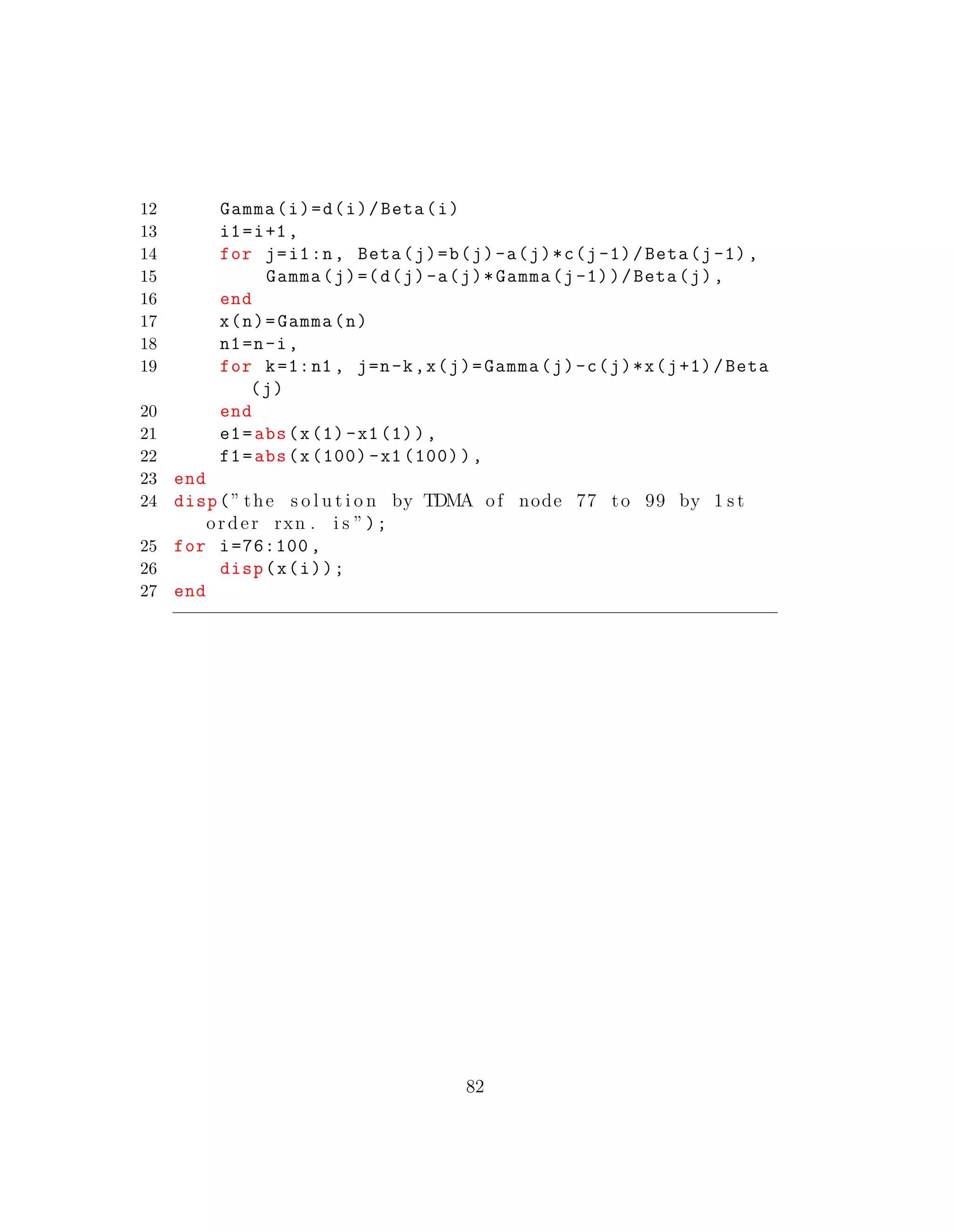
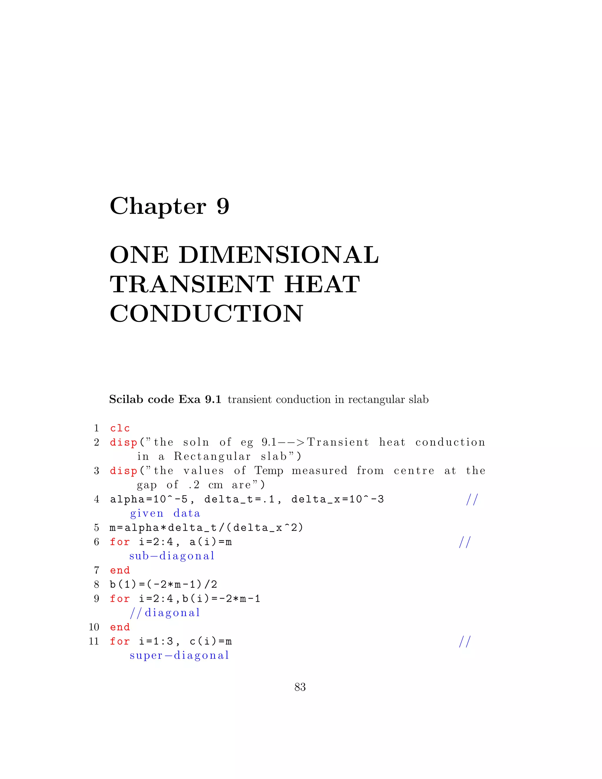
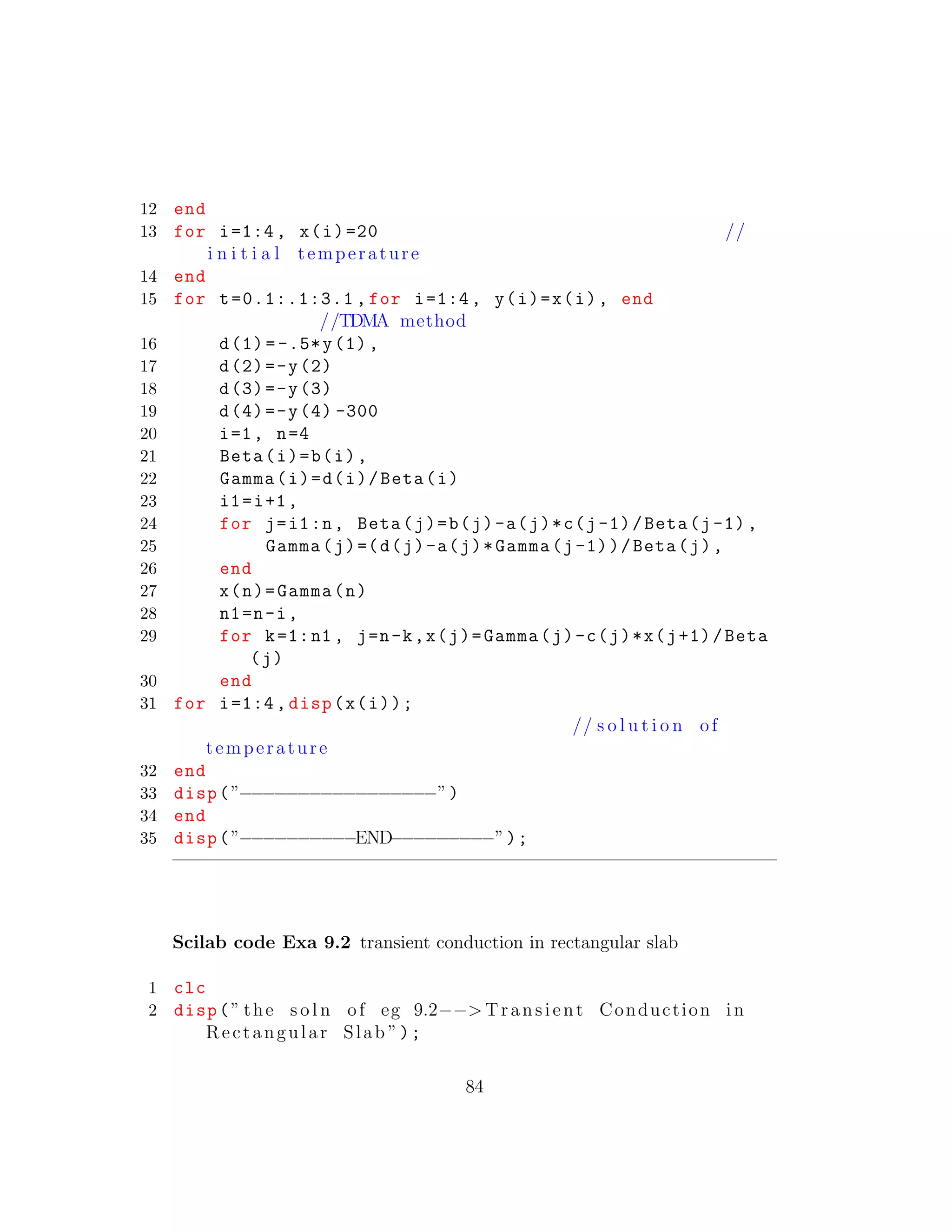
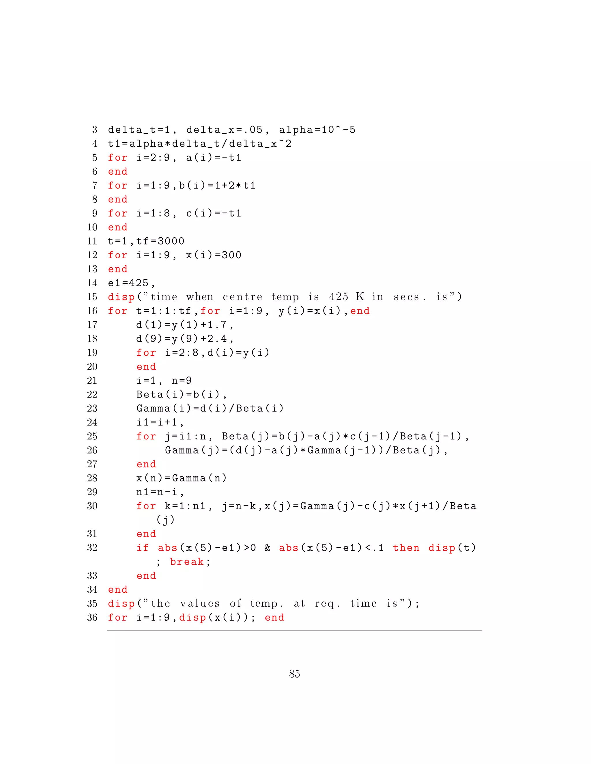
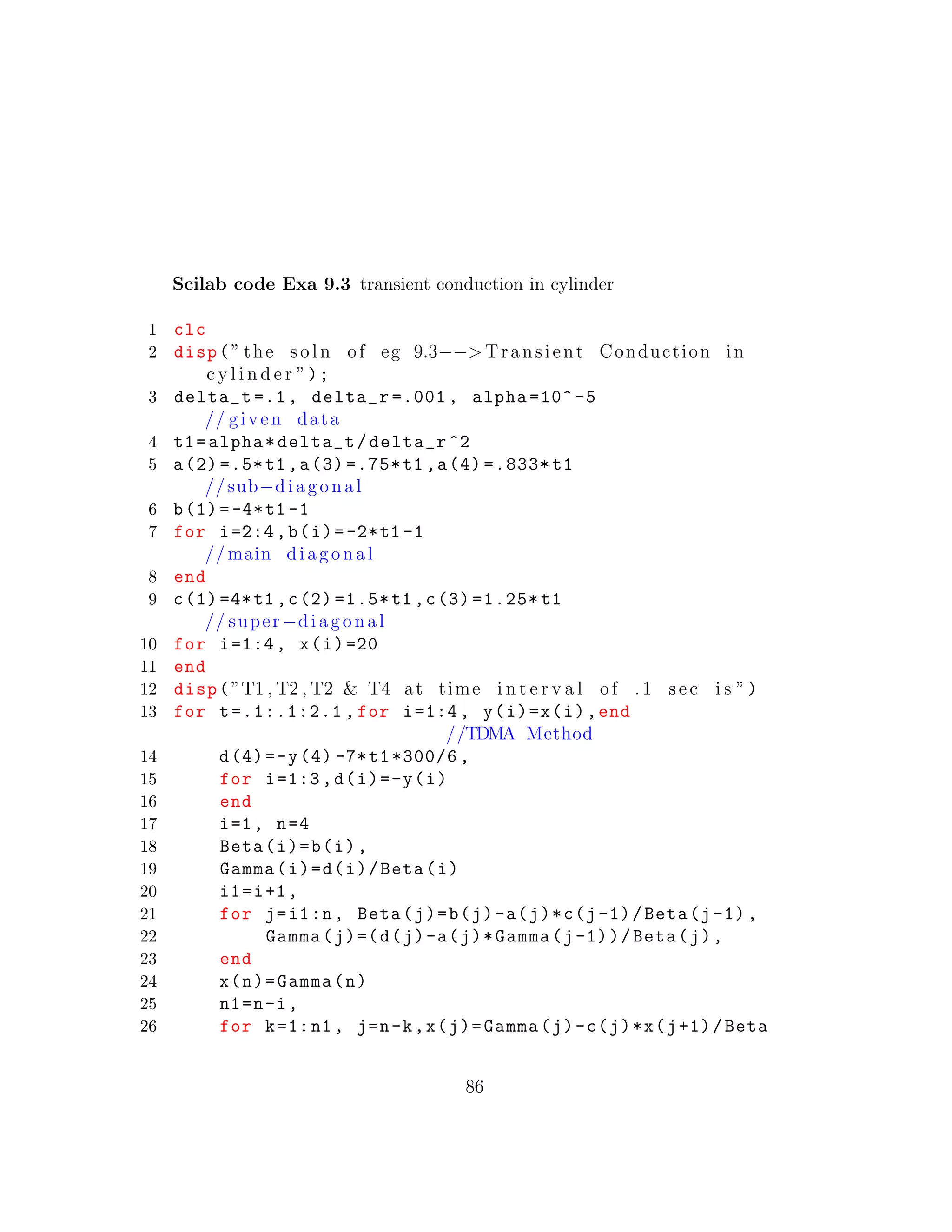
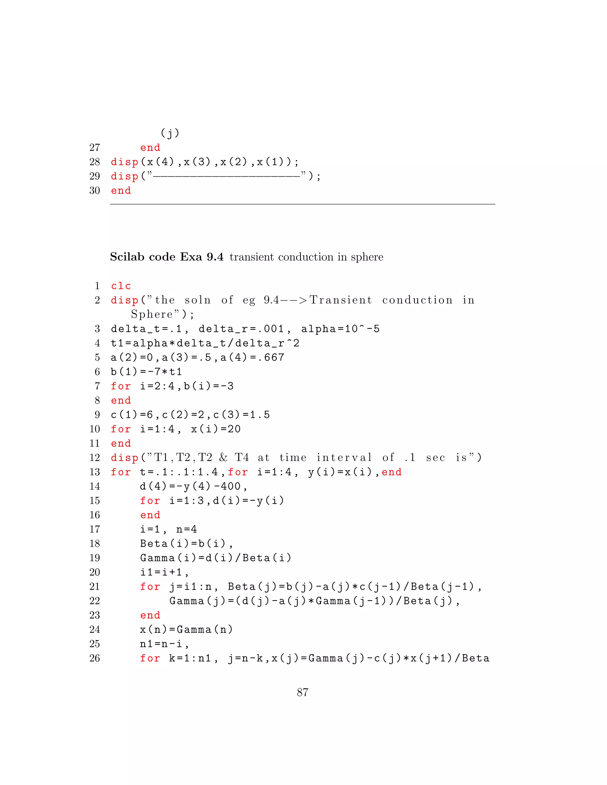
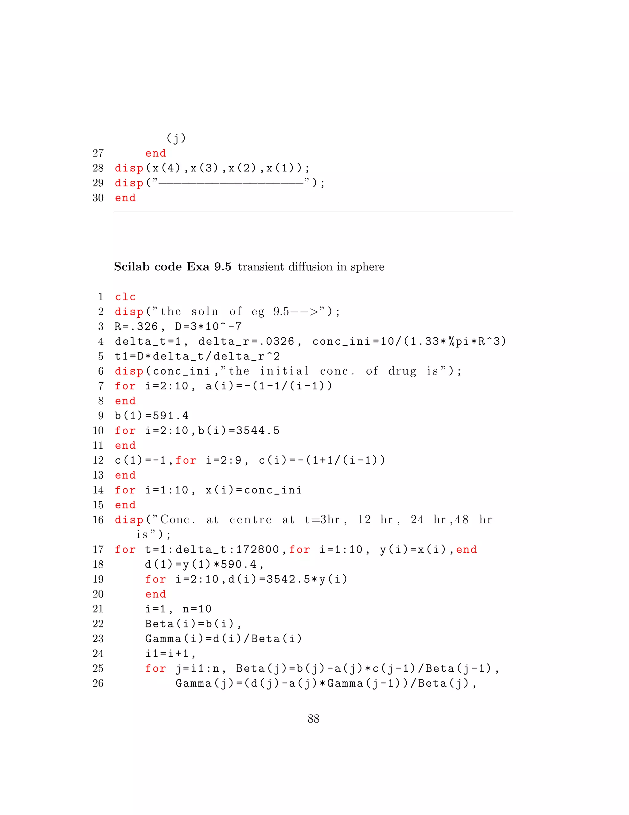
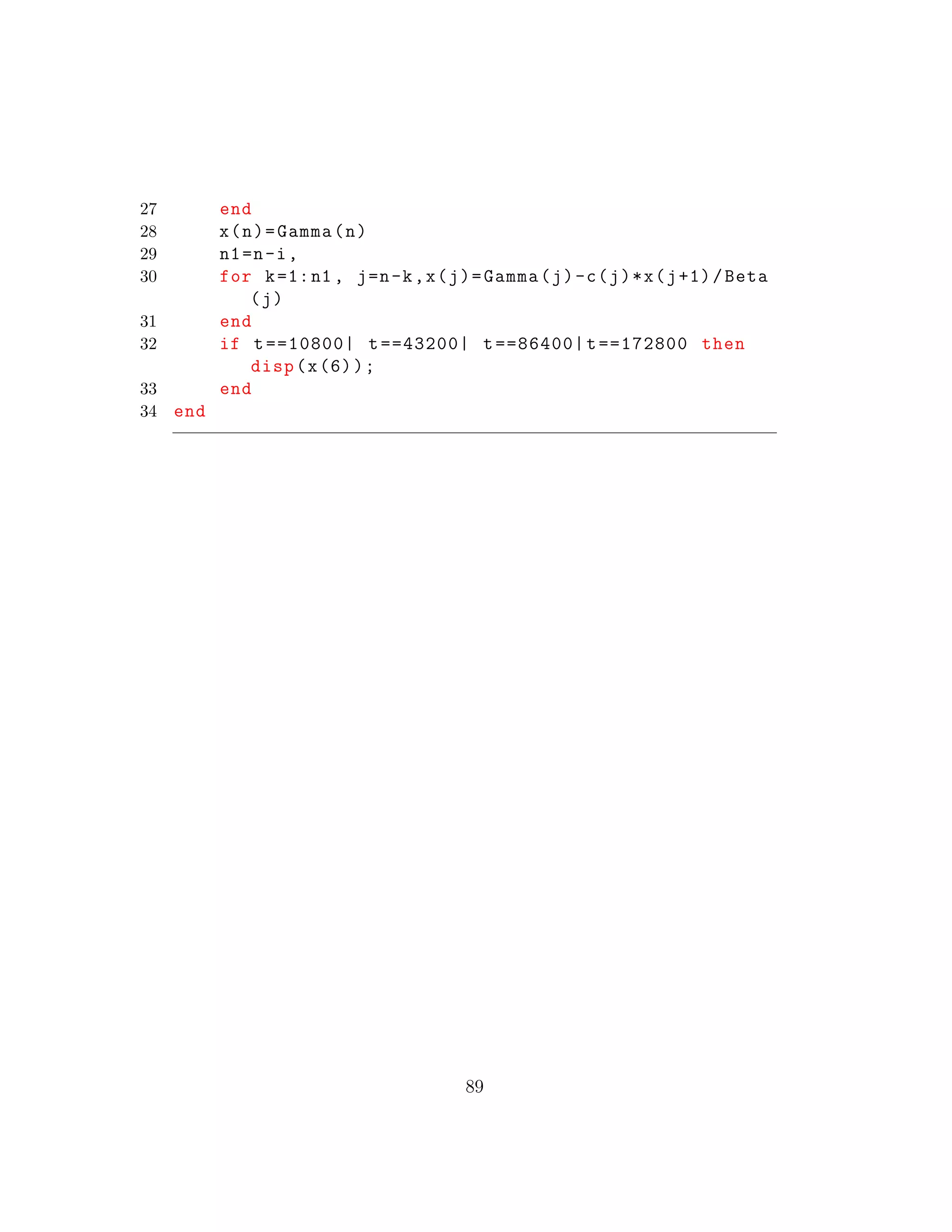
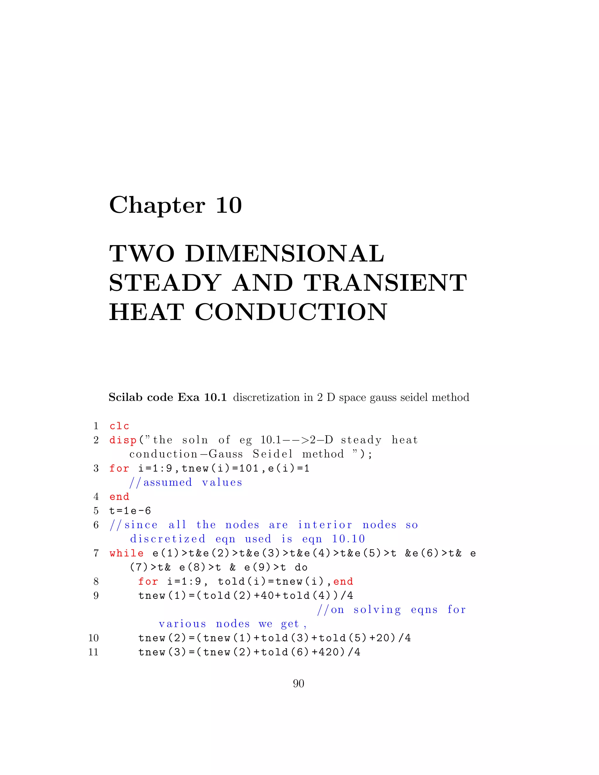
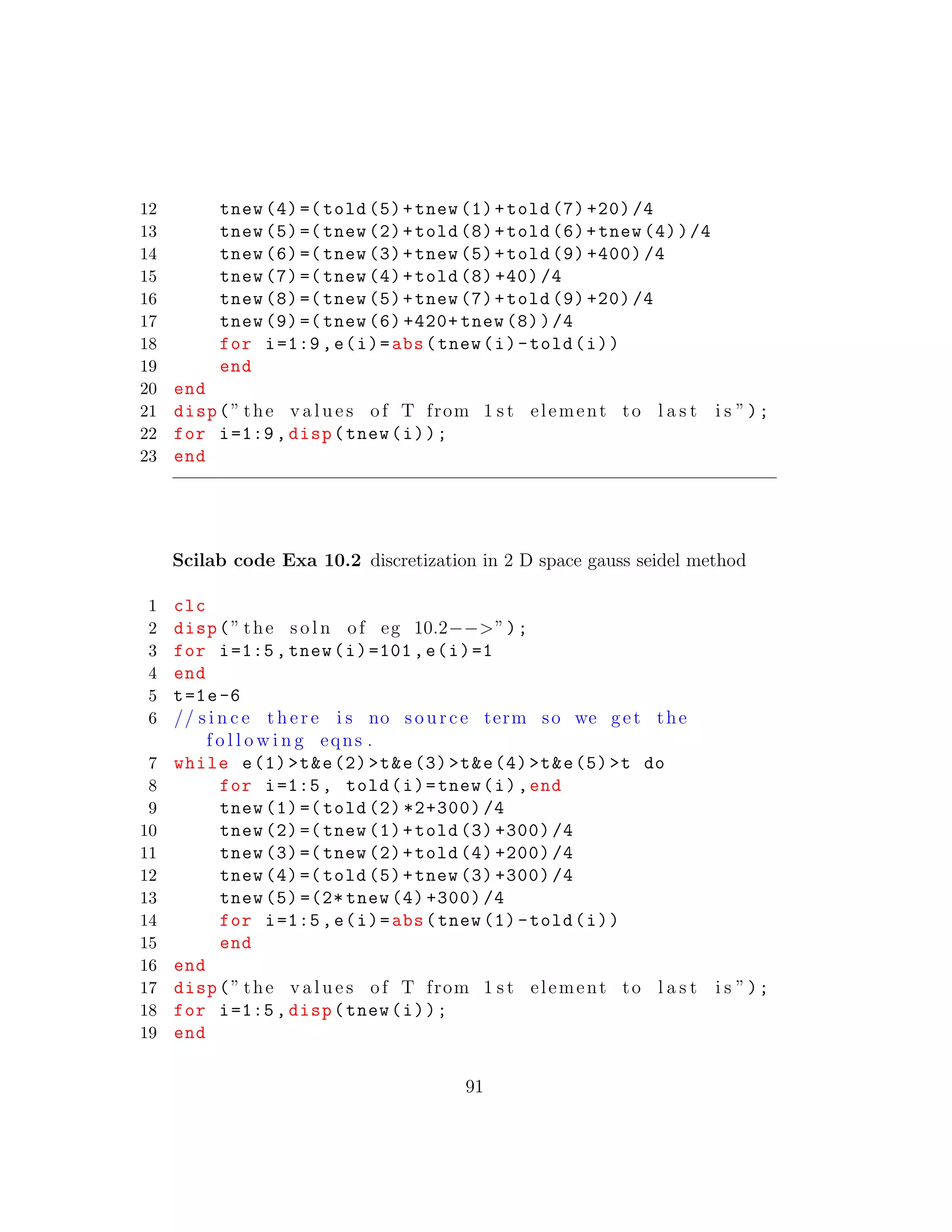
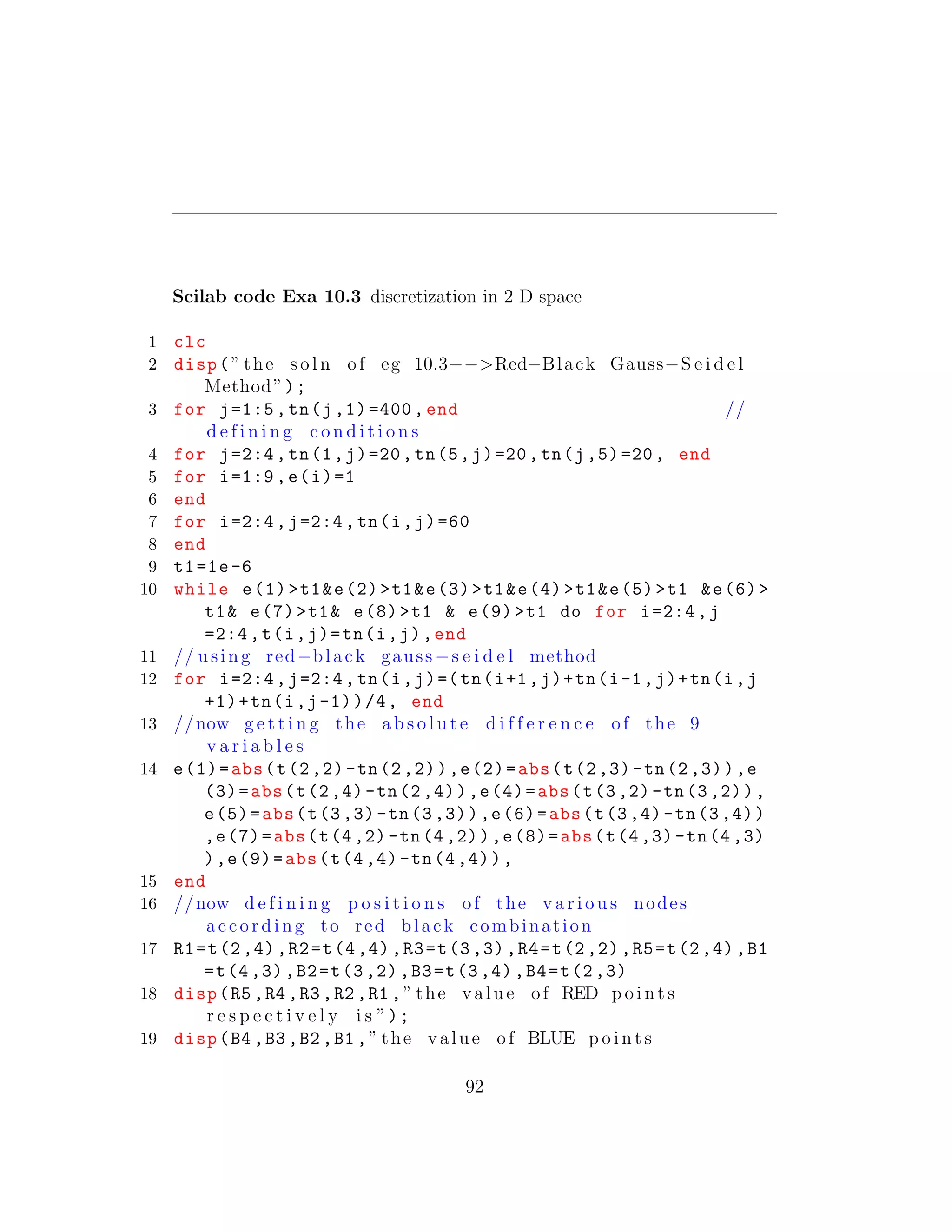
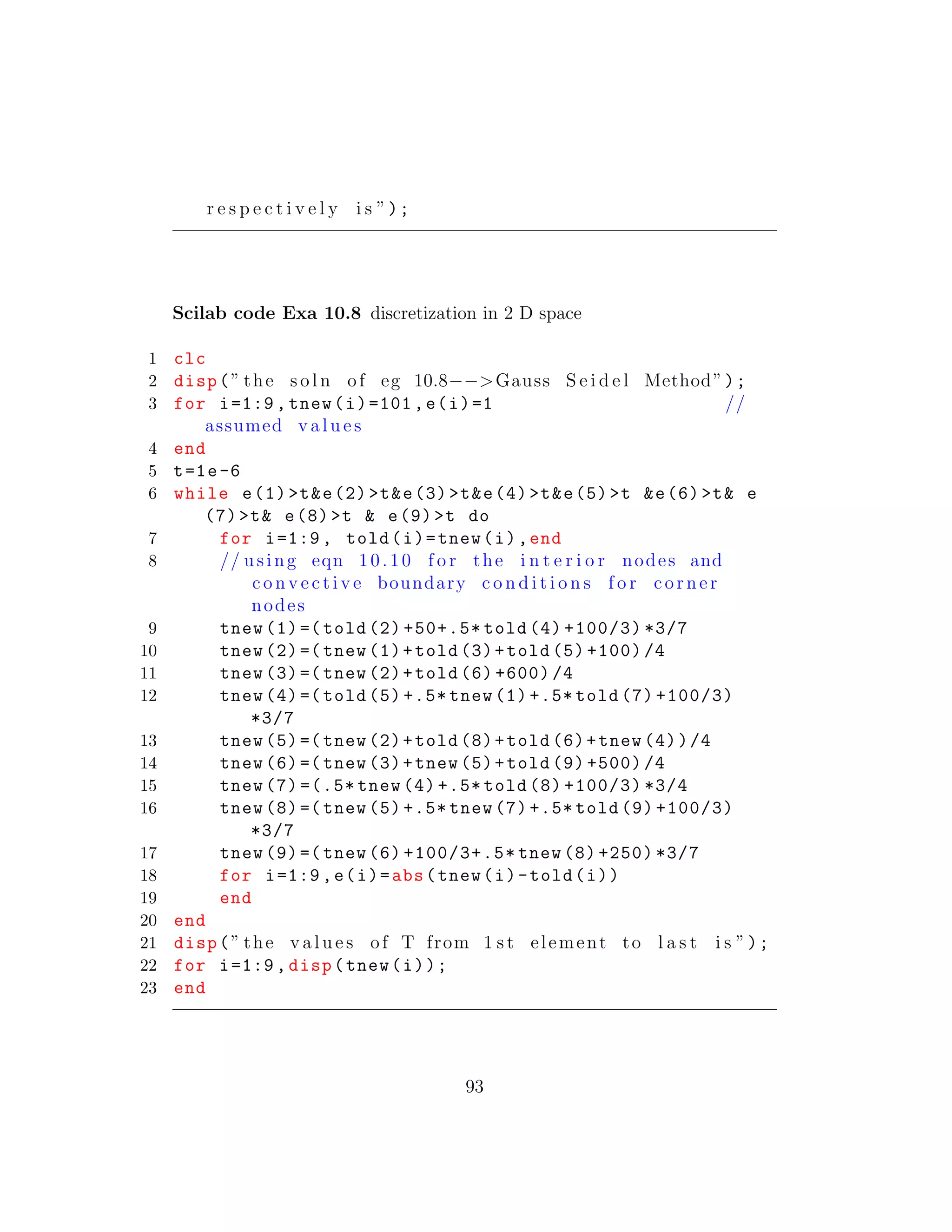
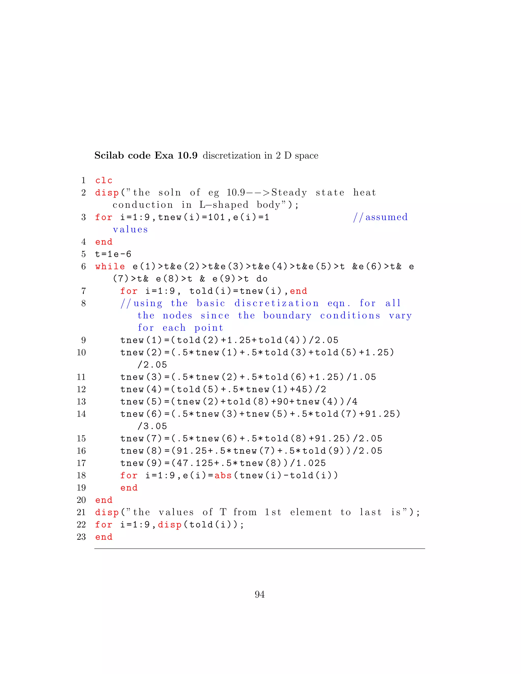
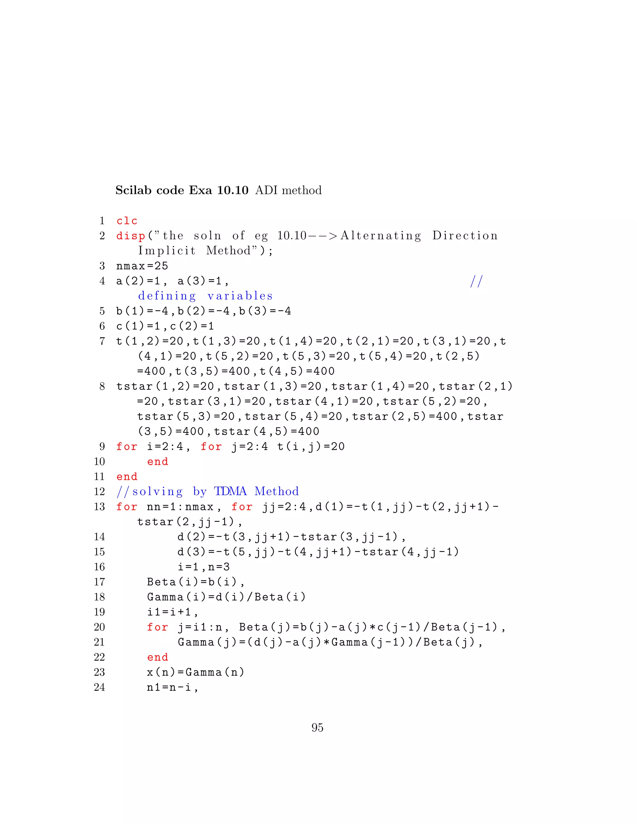
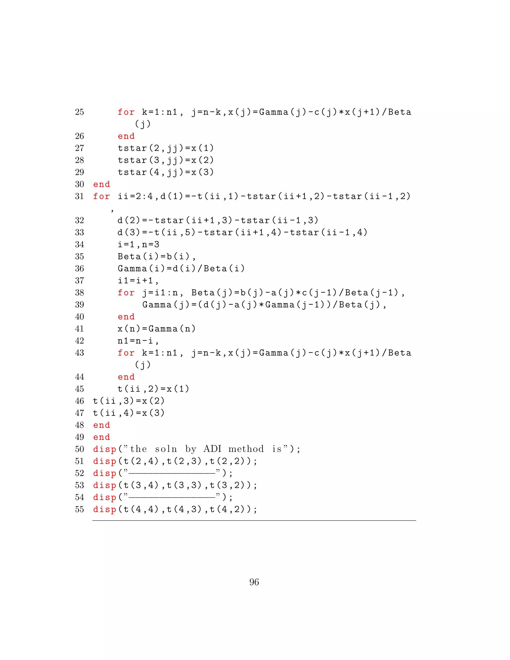
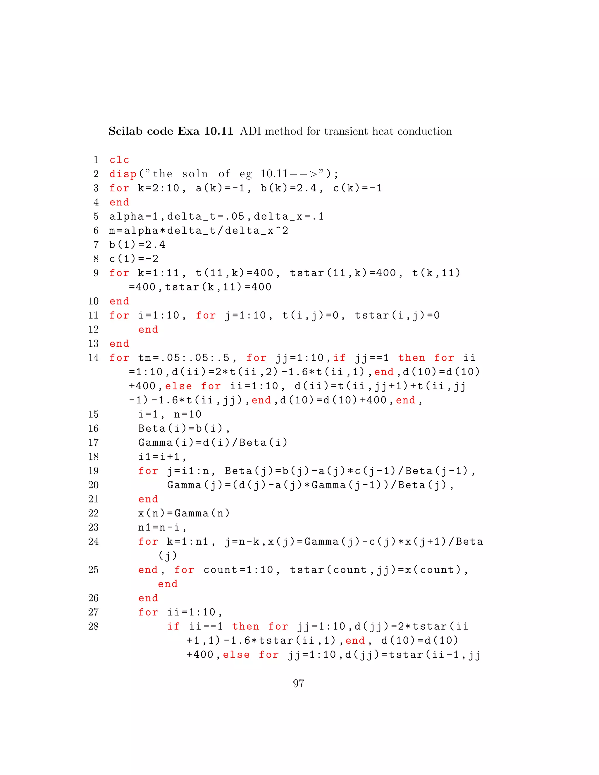
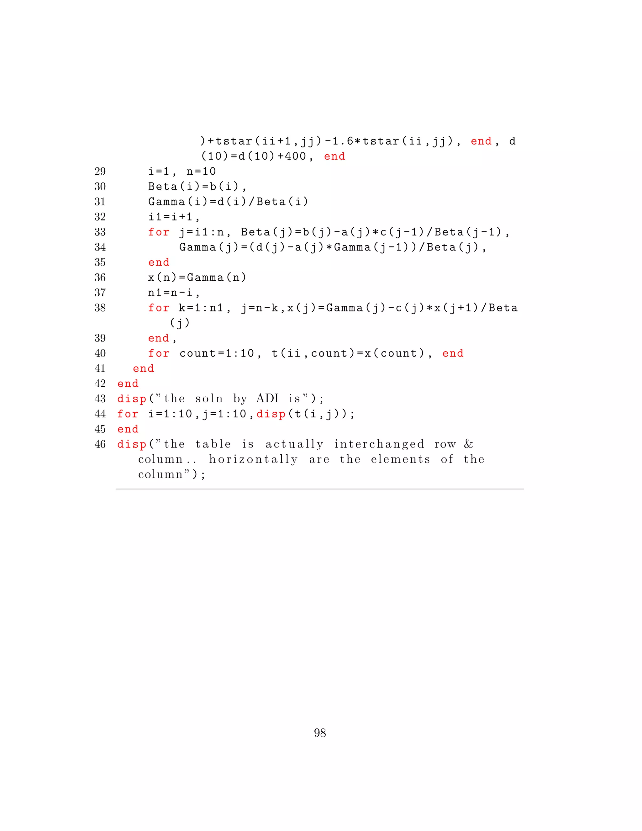

This document contains Scilab codes for solving numerical problems in chemical engineering presented in the textbook "Introduction To Numerical Methods In Chemical Engineering" by P. Ahuja. It includes codes for solving linear algebraic equations using methods like TDMA, Gauss elimination, and Gauss-Seidel. It also contains codes for solving problems in areas like nonlinear algebraic equations, chemical engineering thermodynamics, initial value problems, boundary value problems, and more. The codes are accompanied by explanations of the problems they solve and the relevant examples from the textbook.