Ta bueno

1. INTEGRAL DEFINIDA
El teorema fundamental del cálculo
Dr. Rolando Vásquez

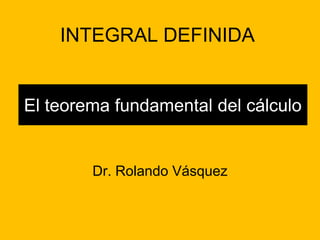
2. El teorema fundamental del cálculo
• Al momento de querer resolver una integral que tenga límites, integrales
definidas o de Riemann, por ser éste matemático uno de los precursores de
este tipo de integrales.
• El enunciado: Sea f una función continua en [a; b]. Entonces,
f (x)dx F(x) F(b) F(a) b
   
a
b
a
donde: a = Límite inferior y b = Límite superior.
Fórmula de Newton-Leibniz.

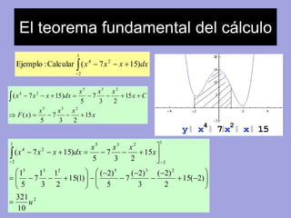
3. El teorema fundamental del cálculo
4
y x
2
7 x
x 15

1
4 2 Ejemplo : Calcular (x 7x x 15)dx


  
2
5 3 2
x x x
      7
  
x
4 2
x x x dx
( 7 15)
5 3 2
x x x
F x
x C
15
    
3 2
7
5
( )
15
3 2
5
5 3 2 5 3 2


1
  7
 
2
1
2
1 5 3 2
2
4 2
1
321
10
15( 2)
( 2)
2
( 2)
7
3
( 2)
5
15(1)
1
2
3
5
15
3 2
7
5
( 7 15)
u
x
x x x
x x x dx


 


 

 






  

 


      
 

4. El teorema fundamental del cálculo
1
4
 
0
1
3
3
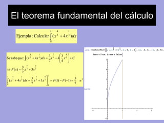
Ejemplo : Calcular (x 4x )dx
2


x x dx x x C
1
3
0
4
3
4
7
4
3
F x x x
  
1 7
3
0
1
3
4
3
3
3
4
3
7
3
1
3
3
3
7
3

3 (1) ( 1)
3
7
( 4 )
3
7
( )
4
4
7
Se sabe que : ( 4 )
x x dx x x F F u
    

  







  



5. ln 2
Ejemplo : Calcular e e dx x x
 
1
2
ln
Log 2
Log
1
2
Exp x Exp x x
Solución
1. Método a emplear: Integración Definida.
2. Regla de integración: Teorema fundamental del cálculo(TFD)
3. Desarrollo:

       e e dx e dx dx x x x
1
 
2ln 2
1
2
ln 2 ln
ln 2
1
2
ln
ln 2
1
2
ln
ln 2
1
2
ln
0
ln 2
2
ln

0.5 1.0 1.5 2.0
1.0
0.8
0.6
0.4
0.2
In[38]:=
Log 2
Log
1
2
x
e
e
x
x
Out[38]= 2 Log 2

6. 3
    
2 Ejemplo : Calcular x 4x 3 dx
1
Solución
1. Método a emplear: Integración Definida.
2. Regla de integración: Teorema fundamental del cálculo(TFD)
3. Desarrollo:
 
1
x x dx x x x

  
     
2
3 2
3
1
3 2
3
1
2
1
4
3
   
2 3
1
3
3 2 3 3 3
3
2 3
3
4 3
u









      
2
In[2]:= ContourPlot y x
4 x 3, x 1, x 3 ,
x, 1, 4 , y, 1, 4 , Axes True, Frame False
Out[2]=
4
3
2
1
1 1 2 3 4
1

7. 2
Ejemplo: 
dx
ln
e
e x x
dx e

d ln
x
   
e e
 
ln(ln ) ln(ln )
ln 2 0.69
ln ln
ln
ln
2
2
2 2
 
x
x
x x
e
e
e
e
e
Solución:
ContourPlot y
1
x Log x
2 4 6 8 10
2
1
1
2
3
4
5
In[68]:=
Exp 2 1
Exp 1
x Log x
x
Out[68]= Log 2
, x Exp 1 , x Exp 2 ,
x, 1, 10 , y, 5, 2 , Axes True,
Frame False

8. Cambio de variable en la integral definida
2
   
( ) ( ( )) ( )
1
t
t
b
a
f x dx f  t  t dt
Ejemplo:
 1

2
2
2 1
2
dx
x
x
1 x2
x2
x, 2, 2 , y, 1, 10 , Axes True,
10
8
6
4
2
ContourPlot y
, x
2
2
, x 1 ,
Frame False
2 1 1 2
In[74]:=
1 1 x2
2
2
x2
x
Out[74]= 1
4

9. 



2 

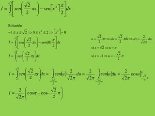
I  sen x senx  dx








 





2
1
2
2 2
 
x x x
       
1 2 0 2 0




2
2
I sen x sen dx






1
2
I sen x dx


 

 







 

 


2
1
2 2
2
2
(0)
2
Solución



2
u  x  du  dx  dx 
du


2

 
2
2
2
x u
si 2
  
x u
si 1
2
2
2
    
2
2
2
    
 
2
I sen x dx sen u du sen u du u
  









2
  

  








2
 

2
 

  





2
cos cos
2
cos
2
2
2
2
2
2
2
2
2
2
1
I

10.  1

2
2
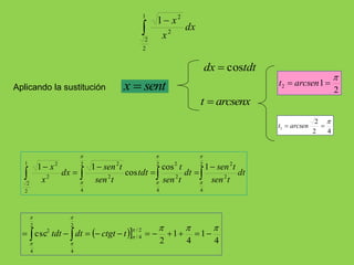
2 1
2
dx
x
x
Aplicando la sustitución sent x 
dx  costdt
t  arcsenx
2
2 4
1

t  arcsen 
2
1 2

t  arcsen 
1 2
2 2
2 2
 sen t
t
2
   

 


4
sen t
2
4
2
4
2
2
2
2
2 cos 1
cos
1 1






dt
sen t
dt
sen t
tdt
sen t
dx
x
x
 
4
  tdt   dt   ctgt  t      1

4
1
2
csc / 2
/ 4
2
4
2
4
2    






11. 3
 
0
1dxx x
Aplicando la sustitución z 1 x 2
dx  2zdz
z  1 x
1 1  z
2 2  z
2
 x  x dx   z  z dz
1
4 2
3
0
1 2 ( )
In[13]:= ContourPlot y x 1 x , x 0, x 3 , x, 1, 5 , y, 1, 7 ,
Axes True, Frame False
Out[13]=
6
4
2
1 1 2 3 4 5

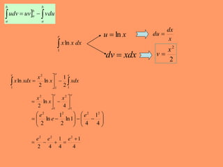
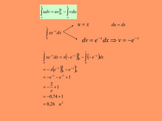
12. Integración por partes
b
    
a
b
b
a udv uv vdu
a
e
x xdx
1
Ejemplo : Calcular ln

In[78]:=
Exp 1
1
x Log x x
Out[78]=
1
4
1
2
In[23]:= ContourPlot y x Log x , x 1, x Exp 1 ,
x, 1, 4 , y, 1, 4 , Axes True, Frame False
x Log x x
Exp 1
1
x Log x x
Out[23]=
4
3
2
1
1 1 2 3 4
1
Out[24]=
x2
4
1
2
2
Log x
x
Out[25]=
1
4
1
2

13. 1

0
arctan xdx x
2
1
arctan
2
2
x
dv xdx v
dx
x
u x du
  

  
1
 




 
1
2 4
arctan
1
1
2
arctan
2
1
1
1
2
arctan
2
2 1
arctan
2
arctan
1
0
1
0
2
1
0
2
1
0
2
1
0
2
2
1
0
1 2
0

  




  







  


dx

 



x x x
x
dx
x
x
x
x
x x
x
x xdx
In[34]:= ContourPlot y x ArcTan x , x 2, x 2 3 ,
x, 4, 4 , y, 4, 4 , Axes True, Frame False
x ArcTan x x
1
x ArcTan x x
0
Out[34]=
4
2
4 2 2 4
2
4
Out[35]=
x
2
ArcTan x
2
1
2
2
ArcTan x
x
Out[36]=
1
4
2

14. b
    
a
b
b
a udv uv vdu
a
e
x x dx
1

ln
x u ln 
dv  xdx
dx
x
du 
2 x
2
v 
e e e

1
   


x xdx
x
x xdx
1 1
2
ln
2
2
1 ln
e e
x
x
x
1
2
1
2
4
ln
2




 



 

2 2 
e
2 2    

 



 
 

1
4
4
1
ln1
2
ln
2
e
e
2 2 2 
4
1
e e 1
e
   
4
2 4

15. b
    
a
b
b
a udv uv vdu
a
x u 
dx du 
x x dv e dx v e     
1
xe dx x  
0
   
x x x
    
xe dx x e e dx
   

x e e
  
1 1
e e
   
  
  
0,74 1
2
1
0
1
0
1
0
1
0
1
0
0,26
1
2
1
u
e
x x

   
 