INFERENTIAL STATISTICS

Inferential Statistics
        provide a means for drawing conclusions about a population given data from a sample
        trying to reach conclusions that extend beyond the immediate data alone
        to make judgments of the probability that an observed difference between groups is a dependable one or that
        might have happened by chance
        Probabilistic estimates involve some error, but inferential statistics provide a framework for making objective
        judgments about their reliability.
        Researchers use inferential statistics to estimate population parameters from sample statistics.

Sampling Distributions
       To estimate population parameters, it is clearly advisable to use representative samples, and probability
       samples are the best way to get representative samples.

        Inferential statistics are based on the assumption of random sampling from populations, an assumption that is
        widely violated.
        Even when random sampling is used, sample characteristics are seldom identical to population characteristics.

Example
    Suppose we had a population of 50,000 nursing school applicants whose mean score on a standardized entrance
      exam was 500 with an SD of 100.
    Suppose we had to estimate these parameters from the scores of a random sample of 25 students.
    Would we expect a mean of exactly 500 and an SD of 100 for this sample?
    Let us the sample mean is 505. If a new random sample were drawn, we might obtain a mean value such as 497.
    The tendency for statistics to fluctuate from one sample to another reflects sampling error.

Sampling error refers to differences between population values (such as the average age of the population) and sample
values (such as the average age of the sample)

So what do we do now!!? If average value computed from a single sample can be erroneous!?

Let’s consider this:
     Consider drawing a sample of 25 students from the population of 50,000, calculating a mean, replacing the
        students, and drawing a new sample.
     Each mean is considered a datum.
     If we drew 10,000 samples, we would have 10,000 means (data points) .
     This distribution could be used to construct a frequency polygon and it is called sampling distribution of the
        mean.

Statistical Inference two techniques:
              1. Estimation of Parameters
              2. Hypothesis Testing

Hypothesis Testing

        Allows objective decisions if results likely reflect chance sample differences or true differences in a population.
        provides objective criteria for deciding whether research hypotheses should be accepted as true or rejected as
        false
        Hypothesis testing is based on rules of negative inference.

        Null hypothesis (Ho) = No
        Alternative hypothesis (H1) = There is
If null hypothesis is rejected, alternative hypothesis is accepted
If null hypothesis is accepted, alternative hypothesis is rejected

Steps in Hypothesis Testing
1. selecting an appropriate test statistic
2. selecting the level of significance
3. computing a test statistic
4. determining the degree of freedom
5. comparing the test statistic to a tabled value

Errors in Hypothesis Testing

Type I Error
   - rejecting a “true” null hypothesis
   - is a false positive conclusion

Type II Error
   - accepting of a “false” null hypothesis
   - is a false negative conclusion

Level of Significance
        Also known as Significance Level
        Researchers control the risk of Type I error by selecting a level of significance
        Pre – decided prior to testing hypothesis to avoid bias
        Referred to as Alpha
        Commonly used level .05 and .01

0.05 sig. level = 100 samples drawn from population, “true” null hypothesis would be rejected 5 times
5% chance of Type 1 error (rejecting a true null)

0.01 sig level = 1 sample out of 100 would the null wrongfully rejected
1 % chance of Type 1 error (rejecting a true null)

0.01 or 0.001 for important decisions

        Lowering risk for Type I error increases risk for Type II error (accepting false null hypothesis)
        also known as the Acceptable Error
        is compared against the Probability of Error (P Value)

P Value - is the estimated probability of rejecting the null hypothesis (H0) of a study question when that hypothesis is
true.

The term significance level (alpha) is used to refer to a pre-chosen probability and the term "P value" is used to indicate
a probability that you calculate after a given study.

Critical Region
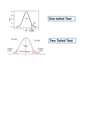
Reject null if test statistics falls at or beyond the limits of the critical region
Not really manually computed

Every statistic there is theoretical distribution to which the computed test stat value is compared
STATISTICALLY SIGNIFICANT = test stat beyond critical limit
Inferential statistics hand out (2)

Inferential statistics hand out (2)

  • 1.
    INFERENTIAL STATISTICS Inferential Statistics provide a means for drawing conclusions about a population given data from a sample trying to reach conclusions that extend beyond the immediate data alone to make judgments of the probability that an observed difference between groups is a dependable one or that might have happened by chance Probabilistic estimates involve some error, but inferential statistics provide a framework for making objective judgments about their reliability. Researchers use inferential statistics to estimate population parameters from sample statistics. Sampling Distributions To estimate population parameters, it is clearly advisable to use representative samples, and probability samples are the best way to get representative samples. Inferential statistics are based on the assumption of random sampling from populations, an assumption that is widely violated. Even when random sampling is used, sample characteristics are seldom identical to population characteristics. Example  Suppose we had a population of 50,000 nursing school applicants whose mean score on a standardized entrance exam was 500 with an SD of 100.  Suppose we had to estimate these parameters from the scores of a random sample of 25 students.  Would we expect a mean of exactly 500 and an SD of 100 for this sample?  Let us the sample mean is 505. If a new random sample were drawn, we might obtain a mean value such as 497.  The tendency for statistics to fluctuate from one sample to another reflects sampling error. Sampling error refers to differences between population values (such as the average age of the population) and sample values (such as the average age of the sample) So what do we do now!!? If average value computed from a single sample can be erroneous!? Let’s consider this:  Consider drawing a sample of 25 students from the population of 50,000, calculating a mean, replacing the students, and drawing a new sample.  Each mean is considered a datum.  If we drew 10,000 samples, we would have 10,000 means (data points) .  This distribution could be used to construct a frequency polygon and it is called sampling distribution of the mean. Statistical Inference two techniques: 1. Estimation of Parameters 2. Hypothesis Testing Hypothesis Testing Allows objective decisions if results likely reflect chance sample differences or true differences in a population. provides objective criteria for deciding whether research hypotheses should be accepted as true or rejected as false Hypothesis testing is based on rules of negative inference. Null hypothesis (Ho) = No Alternative hypothesis (H1) = There is
  • 2.
    If null hypothesisis rejected, alternative hypothesis is accepted If null hypothesis is accepted, alternative hypothesis is rejected Steps in Hypothesis Testing 1. selecting an appropriate test statistic 2. selecting the level of significance 3. computing a test statistic 4. determining the degree of freedom 5. comparing the test statistic to a tabled value Errors in Hypothesis Testing Type I Error - rejecting a “true” null hypothesis - is a false positive conclusion Type II Error - accepting of a “false” null hypothesis - is a false negative conclusion Level of Significance Also known as Significance Level Researchers control the risk of Type I error by selecting a level of significance Pre – decided prior to testing hypothesis to avoid bias Referred to as Alpha Commonly used level .05 and .01 0.05 sig. level = 100 samples drawn from population, “true” null hypothesis would be rejected 5 times 5% chance of Type 1 error (rejecting a true null) 0.01 sig level = 1 sample out of 100 would the null wrongfully rejected 1 % chance of Type 1 error (rejecting a true null) 0.01 or 0.001 for important decisions Lowering risk for Type I error increases risk for Type II error (accepting false null hypothesis) also known as the Acceptable Error is compared against the Probability of Error (P Value) P Value - is the estimated probability of rejecting the null hypothesis (H0) of a study question when that hypothesis is true. The term significance level (alpha) is used to refer to a pre-chosen probability and the term "P value" is used to indicate a probability that you calculate after a given study. Critical Region Reject null if test statistics falls at or beyond the limits of the critical region Not really manually computed Every statistic there is theoretical distribution to which the computed test stat value is compared STATISTICALLY SIGNIFICANT = test stat beyond critical limit