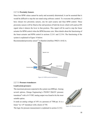
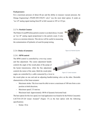
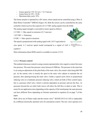
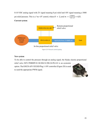
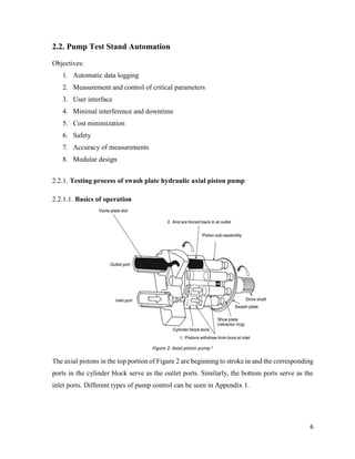
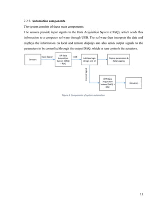
SlideShare a Scribd company logo
1 of 52
Download to read offline
IMPROVEMENT OF THE PUMP TESTING PROCESS AT ATLANTIC
HYDRAULICS, SANFORD, NC
By
Prafulla Kumar Shahi
A project submitted to the Integrated Manufacturing Systems Engineering
Institute of
North Carolina State University
In partial fulfillment of the requirements of the degree of
MASTER OF INTEGRATED MANUFACTURING SYSTEMS
ENGINEERING
Raleigh, North Carolina
2015
Approved by:
Dr. Steven D. Jackson
Advisory Committee Chairman
Director, IMSE Institute
Dr. Thom. J. Hodgson
Professor of Industrial & Systems Engineering
Dr. Yuan-Shin Lee
Professor of Industrial & Systems Engineering
ABSTRACT
SHAHI, PRAFULLA KUMAR. Improvement of the pump testing process at Atlantic
Hydraulics (under the direction of Dr. Steven D. Jackson, IMSE Institute, 2015).
This report describes my internship at Atlantic Hydraulics, which is a pump and cylinder
remanufacturing facility in Sanford, North Carolina. I started work as a Process Improvement
intern in August 2014. My role was to implement focused improvement projects in the pump
testing process to improve the quality and speed of the process. I took on several
responsibilities during my internship, including; providing technical services for pump
assembly, disassembly, testing and troubleshooting.
The major focus of my project and this paper is the automation of the pump testing stand. This
project intended to reduce the large amount of time needed to test hydraulic pumps. The
automation involved sensing and control of different parameters and developing a block
diagram. Every sensor and actuator was chosen to work as a unit with the data acquisition
system and software. The logic was tested for desired results.
Other projects that I worked on included the improvement of the valve lapping process and
preparing the FMEA for the pump testing stand. The existing lapping machine for curved
lapping surfaces was built in-house but was not bring used as it was not lapping to standards.
Using a series of experimental runs, I determined the optimal parameters for bringing the
process up to standards.
ii
DEDICATION
I dedicate this work to my parents and my fiancΓ© for their invaluable support and affection.
iii
ACKNOWLEDGEMENT
I would like to thank Mr. Curt Williams for guiding me throughout my internship program at
Atlantic Hydraulics. He took a serious interest in my work and gave me his valuable inputs
from time to time. He helped me make the choices and recommendations necessary for
implementing this project. His invaluable advice for and suggestions for making improvements
helped me achieve the desired outcome. I would also like to thank several people I met during
the course of planning the project to guide me and give me valuable suggestions without which
I wouldn’t have been able to go through with the project.
I would like to thank Dr. Steven D. Jackson for his continuous help and efforts throughout the
planning and execution of the project. I would also like to thank Dr. Yuan-Shin Lee for
teaching me the concepts of automation that I have used throughout the project. I am also
grateful to Dr. Hodgson, honorable professor of Industrial and Systems Engineering, for
agreeing to be a part of my project committee and Dr. Rick Lemaster for helping me in the
initial phase.
It is also my duty to thank Ms. Nancy Evans for helping me out with all the non-academic
questions and procedures during my status as an IMSEI graduate student.
iv
TABLE OF CONTENTS
List of Tables.........................................................................................................................................vi
List of Figures ......................................................................................................................................vii
List of Abbreviations...........................................................................................................................viii
1. Introduction ........................................................................................................................................1
2. Improvement of the Pump Testing process........................................................................................3
2.1. Improvement of the Pump Testing process.................................................................................4
2.1.1. Background...........................................................................................................................4
2.1.2. Recommendations to workplace optimization and process improvement............................5
2.2. Pump Test Stand Automation......................................................................................................6
2.2.1. Testing process of swash plate hydraulic axial piston pump................................................6
2.2.1.1. Basics of operation ........................................................................................................6
2.2.1.2. Test stand.......................................................................................................................8
2.2.1.3. Testing procedure..........................................................................................................9
2.2.2. Automation components.....................................................................................................12
2.2.3. Input parameters.................................................................................................................13
2.2.4. Output parameters ..............................................................................................................14
2.2.5. Hardware: Data Acquisition system...................................................................................14
2.2.6. Software: LabView.............................................................................................................15
2.2.7. Choice of sensors................................................................................................................15
2.2.7.1. Flow sensors................................................................................................................16
2.2.7.2. Torque transducer........................................................................................................16
2.2.7.3. RPM sensor .................................................................................................................17
2.2.7.4. Proximity Sensors........................................................................................................18
2.2.7.5. Pressure transducers ....................................................................................................18
2.2.7.6. Particle Counter...........................................................................................................19
2.2.8. Choice of actuators.............................................................................................................19
2.2.8.1. RPM control ................................................................................................................19
2.2.8.2. Pressure control ...........................................................................................................20
2.2.8.3. Oil Temperature Control .............................................................................................22
2.2.9. Logic design .......................................................................................................................23
2.2.9.1. User Interface ..............................................................................................................23
2.2.9.2. Data Acquisition..........................................................................................................24
2.2.9.3. RPM sensing................................................................................................................27
v
2.2.9.4. Control.........................................................................................................................27
2.2.9.5. RPM Control ...............................................................................................................29
2.2.9.6. Pressure control ...........................................................................................................31
2.2.9.7. Oil temperature control................................................................................................33
2.2.9.8. Data logging ................................................................................................................34
2.3. Testing.......................................................................................................................................36
2.4. Deliverables...............................................................................................................................36
2.5. Cost............................................................................................................................................37
3. Post-completion................................................................................................................................38
3.1. Takeaways from the project ......................................................................................................38
3.2. Future scope and recommendations ..........................................................................................39
References and Bibliography ...............................................................................................................40
Appendices...........................................................................................................................................41
vi
List of Tables
Table 1: Input parameters.....................................................................................................................13
Table 2: Output Parameters..................................................................................................................14
Table 3: Torque transducer selection ...................................................................................................17
Table 4: Cost calculations ....................................................................................................................37
vii
List of Figures
Figure 1: Current cleaning system..........................................................................................................4
Figure 2: Axial piston pump 2
................................................................................................................6
Figure 3: Hydraulic pump regulator.......................................................................................................7
Figure 4: Pressure-Flow (P-Q) curve .....................................................................................................8
Figure 5: Test Stand Layout ...................................................................................................................9
Figure 6: Pump connected to test stand..................................................................................................9
Figure 7: Pump testing process flow ....................................................................................................11
Figure 8: Components of system automation.......................................................................................12
Figure 9: Input DAQ ............................................................................................................................14
Figure 10: Output DAQ........................................................................................................................14
Figure 11: Flow sensor.........................................................................................................................16
Figure 12: Flow display........................................................................................................................16
Figure 13: Torque transducer ...............................................................................................................16
Figure 14: RPM control mechanism.....................................................................................................18
Figure 15: Pressure sensors ..................................................................................................................18
Figure 16: Particle Counter ..................................................................................................................19
Figure 17: Linear actuator ....................................................................................................................19
Figure 18: Controller............................................................................................................................20
Figure 19: Pressure control piping .......................................................................................................21
Figure 20: Pressure controller ..............................................................................................................22
Figure 21: Pressure control system.......................................................................................................22
Figure 22: Temperature switch.............................................................................................................23
Figure 23: User Interface......................................................................................................................24
Figure 24: Proximity sensing................................................................................................................25
Figure 25: Analog sensing....................................................................................................................25
Figure 26: Data Acquisition .................................................................................................................26
Figure 27: Parameter Control & RPM Sub-VI.....................................................................................28
Figure 28: RPM Control VI..................................................................................................................30
Figure 29: Formula...............................................................................................................................32
Figure 30: Test Run: Ramp UP part.....................................................................................................32
Figure 31: Manual Operation ...............................................................................................................32
Figure 32: Oil Temperature Control.....................................................................................................33
Figure 33: Initial Parameter Entry........................................................................................................34
Figure 34: Plotting Pressure-Flow (P-Q) Curve...................................................................................35
viii
List of Abbreviations
DAQ Data Acquisition System
Hystat Hydrostatic transmission
MCC Measurement Computing
VI Virtual Instrument
NI National Instruments
PWM Pulse Width Modulation
1. Introduction
2
Introduction:
Atlantic Hydraulics is a pump remanufacturing facility in Sanford, North Carolina committed
to being a β€œpartner in the success of its customers”. The company brings failed/worn out
hydraulic pumps and cylinders into the facility. After initial cleaning, disassembly, evaluation,
final cleaning, quoting, approval, assembly, testing and painting, the final product goes out the
line and is delivered to the customer. Several different makes and models of hydraulic pumps
enter the facility, viz. Bosch-Rexroth, Kawasaki, Linde, Eaton, Parker-Dennison, Sauer-
Sundstrand, etc.
In addition to remanufacturing, Atlantic Hydraulics also supplies parts and has an Atlantic
Advantage program in place which offers the exchange program for quick replacement of
pumps/motors. With a one year warranty on remanufactured equipment, good quality of
finished product is very important. The pump line is currently facing several problems, most
of which are related to unavailability of technical information for pump assembly/disassembly
and/or testing.
The major focus of my project and this paper is on the automation of the pump test stand as
part of my process improvement internship with the company that began in August 2014.
3
2. Improvement of the Pump
Testing process
4
2.1. Improvement of the Pump Testing process
2.1.1. Background
The current hydraulic pump remanufacture/repair line consists of the following operations:
The failed/worn pump enters the facility and it is initially tagged, and when the work schedule
permits, it is cleaned and disassembled. Then the pump is cleaned again and evaluated for part
replacement estimates. The quote is sent to the customer and the pump is staged while waiting
for customer approval. Once the approval is received, the pump is cleaned for a last time and
all valves and valve plates lapped. The pump is then assembled, tested and if all parameters
are found to be satisfactory, it is shipped to the customer.
The facility has designated clean, dirty, machining, inventory storage and painting areas which
help keeping the workplace organized.
The current pump line encountered the following problems:
- The pump parts were sometimes not cleaned to standards.
- The valve lapping process was not efficient since curved surface valve plates and
cylinder blocks had to be lapped by hand as the flat surface machine could not be used
Figure 1: Current cleaning system
5
for them. A curved surface lapping machine was built in-house but was not in use since
it was not lapping to standards and caused wastage of lapping plates.
- The assembled pumps required absolutely clean parts but the area surrounding the
workplace was not clean since disassembly and assembly operations were carried out
in the same area.
- A lot of time was wasted in finding out the right connections of the pumps, technical
issues arose out of not knowing the testing procedure or lack of technical information
for the particular make/model of pump. Often the information was available in
electronic format but not readily available due to unorganized information.
- Lack of an automatic data logging method and some parameters were not measured
since the particular sensor was not available. This sometimes resulted in a loss of
valuable data or wrong data being logged.
2.1.2. Recommendations to workplace optimization and process improvement
Many different improvement recommendations were made based on the current situation:
- Using a soda-blasting machine to clean the disassembled pumps before reassembly.
- Improvement in general cleanliness and efficiency of processes in the pump assembly
area using following actions:
o Relocating the pump disassembly workbench to β€œdirty” area.
o Relocating the valve lapping machines to machining area.
- Making design changes to the workbench using powered/hand-operated jigs to hold
pump casing.
- Improve data logging and organization
- Making design changes to test stand to reduce pump connection-disconnection time.
- Automation of the pump test stand.
- Failure Mode Effects analysis of test stand and CNC lathe.
I was assigned the task of planning the test stand automation project and preparing the FMEA
for the test stand and CNC lathe.
6
2.2. Pump Test Stand Automation
Objectives:
1. Automatic data logging
2. Measurement and control of critical parameters
3. User interface
4. Minimal interference and downtime
5. Cost minimization
6. Safety
7. Accuracy of measurements
8. Modular design
2.2.1. Testing process of swash plate hydraulic axial piston pump
2.2.1.1. Basics of operation
Figure 2: Axial piston pump 2
The axial pistons in the top portion of Figure 2 are beginning to stroke in and the corresponding
ports in the cylinder block serve as the outlet ports. Similarly, the bottom ports serve as the
inlet ports. Different types of pump control can be seen in Appendix 1.
7
As the swash plate angle increases, the piston stroke and hence the displacement increases
which causes the flow to increase and vice versa.
Figure 3: Hydraulic pump regulator
The control method used in each pump differs greatly with the make and model number of
the pump. Most of the pumps use a constant horsepower control spool and a pilot control
spool to regulate the position of the lever shown in Figure 3.
Most hydraulic piston pumps operate in a constant power/torque range after a specific system
pressure. The brake power at the shaft of the pump is given by:
π‘ƒπ‘œπ‘€π‘’π‘Ÿ (β„Žπ‘) =
π‘ƒπ‘Ÿπ‘’π‘ π‘ π‘’π‘Ÿπ‘’ (𝑝𝑠𝑖) 𝑋 πΉπ‘™π‘œπ‘€ (π‘”π‘π‘š)
πœ‚ 𝑣 𝑋 1714
……………………………………….. (I)
Where πœ‚ 𝑣 = π‘‰π‘œπ‘™π‘’π‘šπ‘’π‘‘π‘Ÿπ‘–π‘ 𝐸𝑓𝑓𝑖𝑐𝑖𝑒𝑛𝑐𝑦
If the pressure increases beyond a particular value (Break-point pressure), the regulator servo
mechanism changes the flow in inverse proportion to the pressure. This keeps the power
constant, which is the area under the curve. It gives the following curve, referred henceforth as
the P-Q curve, shown in Figure 4 below:
Most of the tested pumps are of tandem type, which consist of two halves operating on the
same shaft independently of each other. The two independent systems are usually included
for bidirectional motion control. The load pressure, flow and pilot pressure are all measured
for the two systems, and for our automation application need to be measured using two
8
sensors for each parameter. The pressure control in each system may be either simultaneous
or independent, depending on several other factors explained in Section 2.2.8.2.
2.2.1.2. Test stand
The test stand consists of a 500 hp electric motor driving a hydrostatic transmission (hystat:
swash plate hydraulic piston pump and motor). Hydrostatic transmission is used instead of a
direct drive to allow for variable load, RPM and torque output depending on the swash plate
angles of the pump and motor. An overview of the system can be seen in Figure 5. A more
detailed hydraulic schematic with the proposed improvements is shown in Appendix 2.
Regulator de-stroke point
(Break point pressure)
Constant Horsepower
control region
Figure 4: Pressure-Flow (P-Q) curve
9
Figure 5: Test Stand Layout
2.2.1.3. Testing procedure
The testing process consists of several steps. If there is any problem at any stage, the whole
process needs to be stopped and checked. Troubleshooting may require disassembly and
replacement of parts, which is expensive and time-consuming. Hence it is critical that the pump
is assembled and mounted correctly in the first try. A detailed process flow is shown in Figure
7.
Figure 6: Pump connected to test stand
10
Procedure:
- Mount the pump on the test stand using the correct mounting flange, make all necessary
connections as shown in Figure 6. Use the right flexible coupling to connect the test
pump to the prime mover.
- Observe safety procedures.
- Start electric motor, increase RPM either clockwise or counterclockwise by coarse
adjustment (hydraulic pump control). As the RPM comes close to the required value,
use fine adjustment (hydraulic motor control). The control method is further explained
in section 2.2.8.1.
- Once the required RPM is achieved, fine tune the pump as per specifications. The
specifications depend on the different type of pumps and their controls.
- Record the P-Q curve at values between 0 and 5000 psi at intervals of 1000 psi, first
upstream, then downstream.
11
Mount Pump to test
stand and
Make all
connections
Start Test Stand
Troubleshoot:
Inspect
Stop
Dismount
Correct
Check for leaks
Set Parameters
Parameters
Correct?
Test P-Q Curve
Parameters
Correct?
StopData Logging
End
Start
Remove connections
and Dismount
YES
NO
YES
NO
NO
YES
Figure 7: Pump testing process flow
12
2.2.2. Automation components
The system consists of these main components:
The sensors provide input signals to the Data Acquisition System (DAQ), which sends this
information to a computer software through USB. The software then interprets the data and
displays the information on local and remote displays and also sends output signals to the
parameters to be controlled through the output DAQ, which in turn controls the actuators.
Sensors
I/P Data
Acquisition
System (DAQ)
+ ADC
LabView logic
design and UI
Display parameters &
Data Logging
O/P Data
Acquisition
System (DAQ) +
DAC
Actuators
ControlSignal
Input Signal USB
Figure 8: Components of system automation
13
2.2.3. Input parameters
The complete list of input parameters desired as tabulated below:
Sr.
No.
Parameter Type Range Unit Nos.
Input
type
1 RPM Tachometer 0-2500 rpm 1 Analog
2 Pilot Pressure 0-1000 psi 2 Analog
3 PPR / RL-T Pressure 0-6000 psi 1 Analog
4 Load Pressure 0-6000 psi 4 Analog
5 Flow Flow 0-200 gpm 4 Analog
6 Case drain Flow 0-30 gpm 1-4 Analog
7 PPR / RL-T Flow 0-30 gpm 1 Analog
8 Case drain Pressure 0-100 psi 1-4 Analog
9 Torque Dynamometer 0-2500 lb-ft 1 Analog
10 Oil Temperature 40-200 deg F 1 Analog
11 Inlet / Feed Pressure Vacuum-100 psi 1 Analog
12 Differential / Load sense Pressure 0-600 psi 1 Analog
13 Particle counter Counter - ppm 2-4 Analog
14 EPPR / solenoid supply Voltage supply
0-1000 mA, 0-24
V
mA,
V
1
Table 1: Input parameters
Based on prior experience, the input values of RPM, Load pressure, Flow, Torque, Oil
temperature and Inlet/Feed pressure are considered critical to running the test process. These
parameters were considered for the project.
14
2.2.4. Output parameters
Sr.
No.
Parameter Type
Actuator
type
Range
Uni
t
Nos
.
Control
method
Outpu
t type
1 RPM
Tachomete
r
Linear 200 mm 2
Complete
control
Analog
2 Pilot Pressure Electric valve 1000 psi 2 Maintain Analog
3 PPR / RL-T Pressure Electric valve 6000 psi 1 Maintain Analog
4 Load Pressure Electric valve 6000 psi 4
Complete
control
Analog
5 Oil
Temperatur
e
Pump - - 1 Maintain Digital
6 Inlet / Feed Pressure Electric valve 100 psi 1 Maintain Analog
7
Differential
/ Load
sense
Pressure Electric valve 600 psi 1 Maintain Analog
8
EPPR /
solenoid
supply
Voltage/
Current
Voltage/
current
source
0-1000
mA, 0-24 V
mA,
V
1 - Analog
Table 2: Output Parameters
Based on experience, the output values of RPM, Load pressure and Oil Temperature are
considered critical to running the test process. These parameters were considered for control.
2.2.5. Hardware: Data Acquisition system
Measurement Computing was chosen as the hardware for
acquiring sensor outputs and providing control signals to
actuators. Two DAQs, one primarily to take analog inputs
and another primarily to provide analog outputs were
chosen for the purpose. I chose more analog inputs/outputs
since most of the controls and sensing was done through
analog signals.
Input DAQ: USB-1608G17
Main features: 16 SE analog inputs, 8 DIO TTL, 2 counter
inputs, 1 timer output. 10/5/2/1 V bipolar input. (Figure 9)
Figure 9: Input DAQ
Figure 10: Output DAQ
15
Output DAQ: USB-310318
Main features: 8 SE analog outputs, 8 DIO, 2 counter inputs, 1 timer output, +/-10VDC output.
(Figure 10)
2.2.6. Software: LabView
LabView, data analysis, measurement and control software from National Instruments was
chosen as the ideal software for developing the logic. Factors affecting the decision were the
level of complexity of the user interface and control parameters and logic design. The most
ideal package for our requirement was the Full Package.
LabView was chosen for several reasons:
- Quick implementation
Learning the software initially takes some effort and is not intuitive for programmers used to
using other languages. But after the initial learning curve, it becomes easier than most other
methods to implement.
- Flexibility for improvement
- Known compatibility with Measurement Computing (MCC) DAQs
- Availability of LabView Universal Library (ULx) Drivers for MCC DAQs
- Availability of online resources for programming
- Dataflow (G) programming language, which provides a more visual style of programming.
The other choices considered were:
- Webtec C2000 Hydraulic Data acquisition system19
- Matlab
2.2.7. Choice of sensors
For our application, since I had already chosen voltage measurement and control DAQs, I
decided to choose sensors with voltage outputs with a maximum range of -10 to +10 VDC for
compatibility.
16
2.2.7.1. Flow sensors
The current system already had two Hedland Flo-tech flow sensors in
place, each with a capacity of 200 GPM. Each flow sensor came with an
individual display unit that converted the frequency output from the
sensor into a digitized display. The display units came without any
analog voltage output capabilities. New flow display units F6600-C-X-
G from Badger Meter4
were used to provide the analog output for use in the
software. This output was taken from the display and used as analog input
for the DAQ.
The display units are β€œmx+B” type with +10V = 200 GPM. Hence a factor of 20 is used to
arrive at the flow value from the voltage value.
The logic for flow measurement is explained in section 2.2.9.2.
2.2.7.2. Torque transducer
An inline torque sensor was observed to be the best method
considering cost and available space. As per our requirements, we
needed to fix one end of the torque sensor to the prime mover motor
and the other end to the test pump using flexible couplings. The
maximum capacity for the torque transducer was estimated based
on the largest torque taken by any pump in the past, which was the Kawasaki K3V280-DTP
pump. The F.L. torque needed by this pump is 1950 N-m. Desirable characteristics:
- 20,000 lbf-in, with a maximum overload capacity of 100%.
- Expected maximum RPM of 2500 in both clockwise and anticlockwise directions
- Open shaft with 5” length and 2.5” diameter.
- -/+10 VDC analog output.
The logic for torque measurement is explained in section 2.2.9.2.
Figure 12: Flow display
Figure 11: Flow sensor
Figure 13: Torque transducer
17
The following options were considered for the torque sensor:
Make Model# torque sensor
Model# Speed
sensor
Additional components
Honeywell 1606-20K 064-LW24368-2 Daytronic 5D78V
Measurement
Specialties, Inc.
CD1140-7, 12-pin
connector
-
Twisted pair shielded cable,
Belkin or equivalent
S. Himmelstein &
Company
MCRT 48006V(2-4)-F-N-A A
Table 3: Torque transducer selection
Based on several factors including cost, linearity, hysteresis, temperature range, temperature
sensitivity, the Measurement Specialties, Inc. CD1140-7 torque transducer15
was
recommended as the ideal choice.
The output signal from the torque transducer is directly proportional β€œmx+B” to the torque. At
zero torque, the voltage signal is zero, while at 20,000 lbf-in, the voltage signal is +/- 10V
depending on the direction of rotation.
2.2.7.3. RPM sensor
The current system already had a tachometer in place, with a maximum measurable value of
3000 rpm. The RPM meter came with an individual display unit which was obsolete and was
not configurable to provide an analog output. The Measurement Specialties, Inc. torque
transducer had a speed pick-up option at an extra cost which provided pulse output at a fixed
rate of 60 pulses per revolution. The value of rotational speed in RPM can be found using
converting the units and using the following formula:
𝑅𝑃𝑀 =
𝑃𝑒𝑙𝑠𝑒 π‘π‘œπ‘’π‘›π‘‘π‘’π‘Ÿ π‘“π‘Ÿπ‘’π‘žπ‘’π‘’π‘›π‘π‘¦
𝐹𝑖π‘₯𝑒𝑑 𝑝𝑒𝑙𝑠𝑒 π‘Ÿπ‘Žπ‘‘π‘’
Thus, the value of RPM turns out to be equal to the frequency counted in Hz, which is displayed
on the monitor.
The frequency, however, is not directly configurable as the speed pickup is a simple magnetic
self-induced type. Due to this, at RPM below 100, the amplitude of the induced voltage is too
low to be detected as significantly different from the noise.
A different method to distinguish frequencies is detailed in section 2.2.9.3.
18
2.2.7.4. Proximity Sensors
Since low RPM values cannot be easily and accurately determined, it can be assumed that it
would be difficult to stop the test stand using software control. To overcome this problem, I
have chosen two proximity sensors, one for each (coarse and fine) RPM control. These
proximity sensors will be fitted at the null position of both the levers which will send an ON
signal when it detects the lever in that position. This signal will be used to stop the linear
actuator for RPM control when the RPM becomes zero. More details about the functioning of
the linear actuator and RPM control in sections 2.2.8.1 and 2.2.9.4. The functioning of the
system is explained in Figure 14 below:
Recommended proximity sensor12
is Hamlin-Littelfuse 59025-1-S-02-A.
2.2.7.5. Pressure transducers
Load/system pressure:
The maximum pressure expected in the system was 6000 psi. Among
several options, Omega Engineering’s PX309-7.5KG5V pressure
transducer9
with a 0-5 VDC analog output was found to be the most
suitable option.
It sends an analog voltage of 10V at a pressure of 7500 psi. It is a
linear β€œmx+B” transducer with a factor of 750.
The logic for pressure measurement is explained in section 2.2.9.2.
Figure 14: RPM control mechanism
Figure 15: Pressure sensors
19
Feed pressure:
For a maximum pressure of about 60 psi and the ability to measure vacuum pressure, the
Omega Engineering’s PX209-30V135G5V valve3
was the most ideal option. It sends an
β€œmx+B” analog signal starting from 0V at full vacuum to 10V at 135 psi.
2.2.7.6. Particle Counter
The Parker iCountPD inline particle counter is an ideal choice. It sends
an β€œmx+B” analog signal proportional to the particle count. It also
serves as a moisture detector. This device will be useful in measuring
the contamination of hydraulic oil used for pump testing.
2.2.8. Choice of actuators
2.2.8.1. RPM control
The RPM control is controlled by a two-way coarse
and fine adjustment. The coarse adjustment handle
controls the angle of the swash plate of the pump of
the hystat transmission, while the fine adjustment
controls the motor of the same. Both the swash plate
angles are controlled by a cable connected by a lever to
the swash plate on one end and an adjusting handle/rotating valve on the other. Desirable
characteristics of the linear actuator:
- Maximum stroke: The lever must be able to move a maximum of 100 mm from a zero
position in both directions.
- Maximum speed: 2-5 mm/sec
- Maximum load: Approximately 100 lb of dynamic horizontal load.
The best option for this low speed, low load application was found to be the Pololu Concentric
LACT10-12V-20 Linear Actuator8
(Figure 17) as the best option with the following
specifications:
- Stroke: 10 in
Figure 16: Particle Counter
Figure 17: Linear actuator
20
- Linear speed @ 12V: 0.5 in/s = 12.7 mm/sec
- Linear force @ 12V: 110 lb
- Maximum duty cycle: 25%
The linear actuator is operated by a DC motor, whose speed can be controlled using a TRex Jr
Dual Motor Controller16
DMC02 (Figure 18). Both the motors can be controlled by the same
controller which receives the respective 0-3.3 VDC analog signals from the DAQ.
The analog signal strength is converted to motor speed as follows:
3.3 VDC => Max speed in extension (12.7 mm/sec)
1.65 VDC => Stationary
0 VDC => Max speed in retraction
The speed is proportional to the analog signal with 1.65 V equivalent to
zero speed. A 3 mm/sec speed would correspond to a signal of 1.65 +
(3.3βˆ’1.65)
12.7
𝑋 3 =
2.0397 𝑉
More information about RPM control is available in section 2.2.9.5.
2.2.8.2. Pressure control
The method of pressure control is using a remote operated pilot valve signal to control the main
line pressure. The main line pressure varies between 0-5000 psi. The pressure in the main line
is set using an adjustment in the pilot body of the main valve, the current value being 600-700
psi. As the remote valve is turned, the spool in the main valve adjusts to maintain the set
pressure, thus opening/closing the main valve. Unlike a typical screw down or proportional
reducing valve or a hydraulic pressure reducing valve, which are both of flow control types,
this is a pressure relief valve, which is entirely dependent on pressure and not the flow. At
pressures beyond the set relief, both valves will allow the full flow to drain to tank. This is
easier for our application since depending on the capacity of the tested pump, the same pressure
can have different flows depending on formula mentioned in equation (I) on page 7 of this
paper.
Both valves are of Parker make and the remote valve11
(R1E02-2512-A1-145) is replaceable
by a different electrically operated valve for automation control. The new valve operates on a
Figure 18: Controller
21
0-10 VDC analog signal with 2V signal meaning 0 psi relief and 10V signal meaning a 5000
psi relief pressure. This is a β€œmx+B” control, where 𝐡 = 2, π‘Žπ‘›π‘‘ π‘š = (
5000
10βˆ’2
) = 625.
Current system:
New system:
To be able to control the pressure through an analog signal, the Hydac electric proportional
relief valve M/N PDB08P-01-M-SS6-N-500-24-PG-8.8 is an economic
option. The EHCD-AP11XXXD Plug 1-10V controller (Figure 20) is used
to send the appropriate PWM signal.
Remote proportional
relief valve
In-line proportional relief valve
Figure 19: Pressure control piping
22
Operation:
When the operator increases or decreases the pressure, the control system (software + DAQ)
sends a signal to the valve controller which actuates the position of the valve depending on the
voltage signal. A higher signal implies a higher relief pressure. The pressure and flow are
measured through sensors and the signals are interpreted by the control system and displayed
both locally and remotely.
Unlike RPM control, pressure is not controlled by feedback, open or closed. More detailed
explanation of the control is provided in section 2.2.9.6.
2.2.8.3. Oil Temperature Control
There are several methods for oil temperature control. One way is to use a temperature sensor
with an analog output to the data acquisition system. The software then compares it with the
set temperature. If the measured temperature is more than 5 Β°F above the set temperature, the
software sends a digital ON signal to start the coolant pump. If the measured temperature
reaches more than 5 Β°F below the set temperature, the software sends a digital OFF signal to
stop the coolant pump.
Figure 20: Pressure controller
Figure 21: Pressure control system
23
Another method is to use a NO (normally open) temperature switch to automatically send an
ON signal to start the pump whenever the temperature is above the set high value. If the
temperature falls below the set low value, the switch turns OFF and stops the pump. More
information in section 2.2.9.4.
The recommended method is the temperature switch for its simplicity of operation and control.
For measuring temperature, a gauge is already available in the system. Recommended
temperature switch is: Omega Engineering14
M/N
TSW-55 (Figure 22) which has a 5A rating or the
TSW-51 which has a 1A rating.
2.2.9. Logic design
The LabView programming language is more visual and uses blocks of code connected
through β€œsoftware wiring” that transfer data. Every block executes only when it has all inputs
available and provides output only when it has executed. Different case structures, loops and
time-based structures are possible. Each block of code is called a VI, or Virtual Instrument.
The major sections of the code are explained below:
2.2.9.1. User Interface
The user interface (Figure 23) was designed to be intuitive and provide accurate displays
through both numeric indicators and gauges. The system helps provide maximum automation
and at the same time is flexible enough to provide sufficient user control and flexibility.
The leftmost column is provided for entering all input parameters. Once all parameters are
entered, the operator presses the β€œSTART” button. The rest of the code then starts. The gauges
on the right show the measurements sensed by the input DAQ and the buttons in the center are
used for control.
Figure 22: Temperature switch
24
Figure 23: User Interface
2.2.9.2. Data Acquisition
A major drawback of the USB input DAQ was that it had only 1 ADC and multiplexer. Since
in the long run, we will have to measure about 10-15 analog parameters, the only way to
measure all parameters is to use a single timing process to measure all parameters or use a
timing process to distinguish the acquisition in each channel. In the former, the DAQ
automatically times the sampling rate so that it is evenly spaced to allow for maximum settling
time and avoiding β€˜ghosting’. Ghosting refers to the situation when a channel that has
particularly high impedance is measured, causing the capacitive component to store high
25
charge. If the next channel sample is taken before the charge is dissipated, it shows the same
value as its predecessor1
.
The maximum acquisition rate in this case is about 250 kS/s.
It can be seen in the code in the form of a single VI called β€œAI Voltage” (Figure 24) taking in
samples from every channel at a particular rate and creating a multidimensional array with
rows as channels and columns as measurement samples. The rows are then split into individual
samples and measured to get individual voltages. These voltages are multiplied by the
respective factors (m) and added by a constant (B) explained in the sections above to get the
corresponding measurements.
The proximity sensors are sensed by digital inputs using the same timing methods (Figure 25).
In Figure 26 we can see how each parameter is separated from a common array and then
processed to arrive at the corresponding value. The values are then displayed through gauges
and numeric indicators. To avoid jumping of the gauges, I have taken a mean of all the
available samples and used that as the displayed value. The corresponding error is displayed
as noise and can be accessed from the user interface. The error value will help in identifying
potential problems, and the need for recalibration of sensors, DAQs or the multipliers. The
data acquisition in Figure 26 is performed every 100 ms.
Figure 25: Analog sensing
Figure 24: Proximity sensing
26
Figure 26: Data Acquisition
27
2.2.9.3. RPM sensing
RPM is measured from the standard speed pickup on-board the torque sensor. It outputs a
pulsating AC RMS type signal to the input DAQ, which is measured through the analog
channel. The frequency is measured by simulating the signal through a Fourier transform. An
inbuilt LabView VI called β€œExtract Single Tone Information.VI” is used for this method
(Figure 27). This is done since the amplitude of the incoming pulse train might be too low at
RPMs below 100 to be measured properly. The signal processing ensures that the amplitude
of noise does not factor significantly in calculating the frequency. This frequency is directly
equal to the RPM and is then sent as the detected frequency in the RPM control sub VI.
2.2.9.4. Control
Similar to the input DAQ, the output DAQ has 2 ADCs, but since we need to control at-least
four analog parameters, the signal to each channel has to be merged and then sent to the
channels (Figure 27). The DAQ automatically times the channels so they interfere minimally
with each other.
Similar to data acquisition, the output signals are sent every 100 ms. Both the systems are part
of the same loop.
28
Figure 27: Parameter Control & RPM Sub-VI
29
2.2.9.5. RPM Control
Refer to Figure 28 for the VI.
The RPM control is a multi-stage operation: If the absolute difference between the set RPM
and the measured RPM is less than 3, there is no control, if the difference is between 3 and 10,
there is fine control. Any difference more than that is controlled using coarse control.
Fine control changes the swash plate angle of the motor part of the hystat transmission, while
the coarse control changes the same for the pump part. As the pump is driving the motor, a
small change in pump flow affects the motor RPM significantly.
The linear actuator chosen is controlled by a controller with a null position of 1.65V. It extends
or retracts if the voltage applied to the controller increases or decreases beyond 1.65V. The
speed of the actuator motor is controlled by PWM supplied by the controller, which is in turn
controlled by the analog signal provided to the controller. The speed is proportional to the
difference of applied voltage from 1.65V. The linear actuator remains in its position if it
receives a constant signal of 1.65V.
The coarse control lever has full scale range of about 200 mm. The fine control lever only
moves in one direction from the fully retracted position with a range of about 100 mm. This is
also the null position of the regulating lever. As per the control logic, if the fine control lever
reaches the null position during operation, it stops in its position and further control is provided
by the coarse control lever.
When the user presses the β€œStart Test Stand” button, the VI sends the appropriate signal to
bring the measured RPM to the correct set value. The appropriate signal is sent using PID
control. The constants of the PID control are chosen to have a low proportional and integral
term and a high derivative term to account for the delayed response of the hydraulic system to
a change in the swash plate angle.
If the user presses the β€œEmergency Stop” or β€œStop Test Stand” button, the VI starts reducing
the RPM to zero while displaying a warning message to not shut off the test stand until it stops
completely. Both levers start moving simultaneously toward their respective null positions.
Above 100 RPM, the coarse lever is controlled using PID control. Below 100 RPM, the
measurement system is not accurate and control is achieved through a constant voltage supply.
When the coarse regulating lever reaches its null position, a final message β€œYou can shut OFF
the test stand now” is displayed and the VI stops.
30
Figure 28: RPM Control VI
31
2.2.9.6. Pressure control
Refer to Figures 29, 30 and 31 for the VI.
The pressure control logic works to attain the following objectives:
- Manually control the system pressure
- Complete a test run to plot the P-Q curve
If a pump has two halves, the operator may choose to control system 1, 2 or both. If it has just
one half, he can either choose system 1 or 2. This choice has been included because the higher
capacity pumps take a lot of power to run. Running tests on the two halves one at a time will
allow the hystat transmission to generate enough torque to increase the pressure to its
maximum rating and test the pump as per requirements.
In manual operation (Figure 31), the operator can control (increase, decrease or zero) the
pressure of any system he wants. Pressure is changed in steps of 0.2V, which is equivalent to
a 100 psi pressure change, which is also the resolution required for system pressure.
In automatic operation (Figure 30), the user can press the β€œStart Test Run” button to start the
test run. The pressure first increases to 5000 psi or the maximum voltage rating in 22 sec using
a ramp up function. It then holds at that pressure for 3.3 sec and then ramps down to zero psi
in 22 sec. The whole run lasts 47.3 sec.
The appropriate signals are sent to the channels through a variable in the main loop (Figure 27:
top part). The maximum voltage signal to be supplied is calculated based on the formula shown
in Figure 29. In the formula, x = Maximum pressure rating of the test pump, and y = Maximum
voltage applied to the pressure control valve.
Unlike RPM control, the pressure control has no feedback since the operator will not need to
go to any particular pressure value. The pressure needs to be only increased or decreased.
32
Figure 31: Manual OperationFigure 30: Test Run: Ramp UP part
Figure 29: Formula
33
2.2.9.7. Oil temperature control
If oil temperature is controlled through the software, it can be made possible through a digital
control VI. The digital signal to switch ON the pump is sent whenever the oil temperature
increases beyond 5 Β°F above the set temperature. The pump is switched OFF whenever the
temperature falls more than 5 Β°F below the set oil temperature.
Figure 32: Oil Temperature Control
34
2.2.9.8. Data logging
All the initial operating and testing parameters entered in the system are immediately recorded
into a new file when the acquisition system is first started (Figure 33).
Figure 33: Initial Parameter Entry
During the test run explained in the previous section, the system logs the data required for the
P-Q curve and plots the curve for future reference. It takes 10 samples while ramping up, each
2.2 sec apart, 1 sample at the high voltage level, and 10 more samples while ramping down,
equally spaced (Figure 34).
It automatically takes into account the operator choice regarding controlling a particular half
or both of the test pump.
35
Figure 34: Plotting Pressure-Flow (P-Q) Curve
36
2.3. Testing
The system functions correctly when independent analog signals are applied to the input
channels. The outputs are correspondingly measured and have been found to be correct.
Due to the unavailability of sensors and actuators at the time of writing this paper, an actual
test cannot be performed with the sensor. When actual hardware is available, the system can
be tested and the calibration parameters can be specified with greater accuracy.
2.4. Deliverables
Due to long lead times, the recommended sensors and actuators could not be made available
in time for testing the software and implementing the project. However, the code has been
tested and seen to work satisfactorily. From here, it is only a matter of time before the required
hardware becomes available, and is installed into the system and further development,
integration and troubleshooting can take place.
37
2.5. Cost
The major focus in choosing the sensors, actuators, DAQs and the software was on minimizing
cost and maximizing efficiency.
The cost chart for the project is given below:
Sr.
No.
Name Make Model No. Unit cost Nos. Cost
1
DAQ
Measurement
Computing
USB 3103 349.00
1 349.00
2
DAQ
Measurement
Computing
USB 1608G 399.00
1 399.00
3 1K Potentiometer - 235.00 1 6.99
4
Feed Pressure
sensor
Omega
Engineering PX209-30V135G5V
235.00 1
235.00
5 Proximity sensor Hamlin-Littelfuse 59025-1-S-02-A 4.48 2 8.96
6 Linear Actuator Pololu
Concentric LACT10-
12V-20
89.95 2
179.90
7 Trex Jr Controller Pololu DMC02 59.95 1 59.95
8
Torque sensor
Measurement
Specialties
CD1140-7 6757.34
1 6757.34
9
Speed sensor
Measurement
Specialties
-
604.69 1 604.69
10
Torque cabling
Measurement
Specialties
-
0.00 1 0.00
11
Speed cabling
Measurement
Specialties
-
0.00 1 0.00
12
Load Pressure
sensor
Omega
Engineering PX309-7.5KG5V 225.00 2 450.00
13
Temperature
switch
Omega
Engineering
TSW-55
170.00 1 170.00
14 Flow display 1 Badger Meter 600.00 1 600.00
15 Flow display 2 Badger Meter 500.00 1 500.00
16 Particle counter Parker iCount PD 0.00
17 LabView
National
Instruments
Full Package
2999.00 1 2999.00
18
Pressure relief
valve
Hydac
PDB08P-01-M-SS6-
N-500-24-PG-8.8 600.00 2 1200.00
19
Pressure valve
controller
Hydac
EHCD-AP11XXXD
Plug 1-10V 100.00 2 200.00
Total Cost 14719.83
Table 4: Cost calculations
38
3. Post-completion
3.1. Takeaways from the project
I learned much from the project, with respect to practical industrial automation applications.
Since this project began from scratch, it was crucial to set the right foundation to be built upon
on future upgrades. I learned a lot about hardware operations and data acquisition.
Challenges:
The biggest challenge was choosing the right hardware: Sensors, Actuators, DAQs and the
software. Through recommendations from Dr. Jackson, Curt and other people from industry, I
chose LabView and the consequent decisions were very much dependent on my previous
choices. A lot of different types of sensors and actuators were available in the market and while
searching for my application, I learned of several different methods of sensing and control that
will be undeniably important in the future. I learned a lot about LabView and its data flow (G
language) programming structure. Using the software also made me consider the importance
of choosing the right parameters for calibrating the sensors.
Throughout my internship I was exposed to industrial hydraulics, and it was necessary to stay
informed about all the different components and engineering techniques used in hydraulic
design.
As a technical service engineer, I learned a lot about the axial piston pump and its operations,
regulation, control and testing methods.
39
3.2. Future scope and recommendations
There are a lot of potential improvements in the project. I designed he system to have minimal
interference with the regular operation of the test stand. In fact, most of the upgrades and
installations can be finished with less than an hour of downtime, which is crucial considering
the fact that this is a low volume but very high processing time application. The system is
flexible and it can be easily upgraded, with additional sensing and control installations and
upgrades. The code can be easily modified and implemented accordingly. I have included
several safety considerations while programming the code so as to reduce mistakes by the
operator as much as possible.
In the future, upgrades need to be considered based on priority level. The sensing parameters
needed to be included first are pilot pressure, proportional reducing pressure, case drain flow,
pilot flow, etc. Important control parameters are feed pressure, differential pressure and pilot
pressure.
It will be important to standardize testing procedures as much as possible to ensure as little
error and processing time as possible. Proper documentation of knowledge and lessons learned,
and testing procedures are important to achieve an error-proof system, especially due to the
wide range of pump types serviced in the facility. It is important to include more testing cases
and procedures for pumps of different brands, viz., Kawasaki, Bosch-Rexroth, Linde, Eaton,
Sauer-Danfoss. Each pump has a different method of control as mentioned in appendix 1.
In order to debug parts of the code, it is important to measure the error consistently, prepare a
diagnostics module, and note inconsistencies in performance and make corrections as early as
possible.
Overall, after the basic sensing and control mentioned in this paper are put into use, a stepwise
approach, tackling one parameter at a time would serve best in order to achieve the best results.
40
References and Bibliography
1. DAQ multi-channel acquisition (n.d.)
http://digital.ni.com/public.nsf/allkb/73CB0FB296814E2286256FFD00028DDF
2. Doddannavar, Ravi, Andries Barnard, and Jayaraman Ganesh. "Chapter 3. Hydraulic
Pumps." Practical Hydraulic Systems: Operation and Troubleshooting for Engineers
and Technicians: Operation and Troubleshooting for Engineers and
Technicians. Newnes, 2005. 56. Web. 15 Mar. 2015.
3. Feed pressure sensor (n.d.): http://www.omega.com/pptst/PX209_PX219.html
4. Flow display units (n.d.): www.badger-meter.com
5. LabView forums (n.d.) forums.ni.com
6. Learn data acquisition (n.d.) http://www.ni.com/academic/students/learn-daq/
7. Learn LabView (n.d.) http://www.ni.com/academic/students/learn-labview/
8. Linear actuator (n.d.): https://www.pololu.com/product/2310
9. Load pressure sensor (n.d.): http://www.omega.com/pptst/PX309-5V.html
10. National Instruments - Labview hands-on campus workshop seminar manual
11. Proportional pressure relief valve (n.d.):
http://www.hydac.com/de-en/products/valves/proportional-valves/proportional-
pressure-relief-valves/pdb08p/show/Overview/index.html
12. Proximity sensors (n.d.):
http://www.mouser.com/ProductDetail/Hamlin-Littelfuse/59025-1-S-02-
A/?qs=sGAEpiMZZMs3uAJYYmvlK4xn%2fdk6jSibtd%252brXCgBLaU%3d
13. Rohner, Peter - Industrial Hydraulic Control
14. Temperature switch (n.d.): http://www.omega.com/pptst/TSW.html
15. Torque transducer (n.d.): meas-spec.com.cn/downloads/CD1140.pdf
16. TRex Jr Controller (n.d.): https://www.pololu.com/product/767
17. USB input DAQ (n.d.): http://www.mccdaq.com/usb-data-acquisition/USB-
1608G.aspx
18. USB output DAQ (n.d.): http://www.mccdaq.com/usb-data-acquisition/USB-
3103.aspx
19. Webtec (n.d.): http://www.webtec.com/en/productgroup/ISDA_C2K
41
Appendices
42
Appendix:
1. Types of Pumps, Hydraulic, swash plate type:
1. Open loop
2. Closed loop
Components in different types of control in pumps:
1. Load sense and pressure compensator type
a. With compensator
b. Without compensator
c. Load sense
2. With/without cut-off valve (breakpoint pressure)
3. With/without PPR valve – needs external pilot signal
4. With/without charge pump
5. With/without manual/handle
43
2. Current Hydraulic schematic of the Test stand with proposed improvements:
1. Pressure Sensor
2. Particle Counter
3. Temperature Sensor
4. Remote pressure relief v/v
5. Torque & RPM sensor
6. RPM control
1, 2 & 3
4
5
6

More Related Content

Similar to IMSE report-Prafulla Shahi

Research Project
Research ProjectResearch Project
Research Project
Andisiwe Beja
Β 
THESIS - Ryan Caetano Thesis Submission
THESIS - Ryan Caetano Thesis SubmissionTHESIS - Ryan Caetano Thesis Submission
THESIS - Ryan Caetano Thesis Submission
Ryan Caetano
Β 
Report for WTS Placement
Report for WTS PlacementReport for WTS Placement
Report for WTS Placement
Aiden Cavallero
Β 
Amed Resume[1]
Amed Resume[1]Amed Resume[1]
Amed Resume[1]
aayubi
Β 
2014A1PS212U-Final-PS1-MOALAJAH
2014A1PS212U-Final-PS1-MOALAJAH2014A1PS212U-Final-PS1-MOALAJAH
2014A1PS212U-Final-PS1-MOALAJAH
Taqdees Wadekar
Β 
PhD Thesis - Seyed Reza (Shauheen) Etminan
PhD Thesis - Seyed Reza (Shauheen) EtminanPhD Thesis - Seyed Reza (Shauheen) Etminan
PhD Thesis - Seyed Reza (Shauheen) Etminan
Shauheen Etminan, PhD
Β 
INL-EXT-16-39808 CBP_ Design_Guidance
INL-EXT-16-39808 CBP_ Design_GuidanceINL-EXT-16-39808 CBP_ Design_Guidance
INL-EXT-16-39808 CBP_ Design_Guidance
Johanna Oxstrand
Β 
Pascal Harper CV Linkedin ver 2
Pascal Harper CV Linkedin ver 2Pascal Harper CV Linkedin ver 2
Pascal Harper CV Linkedin ver 2
Pascal Harper
Β 
Ampiire Derrick Intern Report 2015 with Alliance Consultants Ltd
Ampiire Derrick Intern Report 2015 with Alliance Consultants LtdAmpiire Derrick Intern Report 2015 with Alliance Consultants Ltd
Ampiire Derrick Intern Report 2015 with Alliance Consultants Ltd
Derrick Ampiire
Β 
Bw resume 2013 share
Bw resume 2013 shareBw resume 2013 share
Bw resume 2013 share
Brian Wilson
Β 
WU Requirements for High Reliability In Healthcare Discussion.docx
WU Requirements for High Reliability In Healthcare Discussion.docxWU Requirements for High Reliability In Healthcare Discussion.docx
WU Requirements for High Reliability In Healthcare Discussion.docx
write5
Β 
Reliability based design and acceptance protocol for driven piles
Reliability based design and acceptance protocol for driven pilesReliability based design and acceptance protocol for driven piles
Reliability based design and acceptance protocol for driven piles
AlexASquare1
Β 
Wind Tunnel Based Anemometer Testing Facility
Wind Tunnel Based Anemometer Testing FacilityWind Tunnel Based Anemometer Testing Facility
Wind Tunnel Based Anemometer Testing Facility
Benson Gilbert
Β 
35819303-MIT
35819303-MIT35819303-MIT
35819303-MIT
Roland Ayala
Β 

Similar to IMSE report-Prafulla Shahi (20)

Research Project
Research ProjectResearch Project
Research Project
Β 
Leininger_umd_0117N_16271
Leininger_umd_0117N_16271Leininger_umd_0117N_16271
Leininger_umd_0117N_16271
Β 
THESIS - Ryan Caetano Thesis Submission
THESIS - Ryan Caetano Thesis SubmissionTHESIS - Ryan Caetano Thesis Submission
THESIS - Ryan Caetano Thesis Submission
Β 
An Application Of Value Stream Mapping To Reduce Lead Time And WIP In A Make-...
An Application Of Value Stream Mapping To Reduce Lead Time And WIP In A Make-...An Application Of Value Stream Mapping To Reduce Lead Time And WIP In A Make-...
An Application Of Value Stream Mapping To Reduce Lead Time And WIP In A Make-...
Β 
Combined_Doc
Combined_DocCombined_Doc
Combined_Doc
Β 
Report for WTS Placement
Report for WTS PlacementReport for WTS Placement
Report for WTS Placement
Β 
Final
FinalFinal
Final
Β 
Amed Resume[1]
Amed Resume[1]Amed Resume[1]
Amed Resume[1]
Β 
2014A1PS212U-Final-PS1-MOALAJAH
2014A1PS212U-Final-PS1-MOALAJAH2014A1PS212U-Final-PS1-MOALAJAH
2014A1PS212U-Final-PS1-MOALAJAH
Β 
PhD Thesis - Seyed Reza (Shauheen) Etminan
PhD Thesis - Seyed Reza (Shauheen) EtminanPhD Thesis - Seyed Reza (Shauheen) Etminan
PhD Thesis - Seyed Reza (Shauheen) Etminan
Β 
Agile Business Continuity Planning Using Business Process Modeling Notation
Agile Business Continuity Planning Using Business Process Modeling NotationAgile Business Continuity Planning Using Business Process Modeling Notation
Agile Business Continuity Planning Using Business Process Modeling Notation
Β 
INL-EXT-16-39808 CBP_ Design_Guidance
INL-EXT-16-39808 CBP_ Design_GuidanceINL-EXT-16-39808 CBP_ Design_Guidance
INL-EXT-16-39808 CBP_ Design_Guidance
Β 
Pascal Harper CV Linkedin ver 2
Pascal Harper CV Linkedin ver 2Pascal Harper CV Linkedin ver 2
Pascal Harper CV Linkedin ver 2
Β 
Ampiire Derrick Intern Report 2015 with Alliance Consultants Ltd
Ampiire Derrick Intern Report 2015 with Alliance Consultants LtdAmpiire Derrick Intern Report 2015 with Alliance Consultants Ltd
Ampiire Derrick Intern Report 2015 with Alliance Consultants Ltd
Β 
Bw resume 2013 share
Bw resume 2013 shareBw resume 2013 share
Bw resume 2013 share
Β 
127320468-MIT
127320468-MIT127320468-MIT
127320468-MIT
Β 
WU Requirements for High Reliability In Healthcare Discussion.docx
WU Requirements for High Reliability In Healthcare Discussion.docxWU Requirements for High Reliability In Healthcare Discussion.docx
WU Requirements for High Reliability In Healthcare Discussion.docx
Β 
Reliability based design and acceptance protocol for driven piles
Reliability based design and acceptance protocol for driven pilesReliability based design and acceptance protocol for driven piles
Reliability based design and acceptance protocol for driven piles
Β 
Wind Tunnel Based Anemometer Testing Facility
Wind Tunnel Based Anemometer Testing FacilityWind Tunnel Based Anemometer Testing Facility
Wind Tunnel Based Anemometer Testing Facility
Β 
35819303-MIT
35819303-MIT35819303-MIT
35819303-MIT
Β 

More from Prafulla Kumar Shahi

ISE716 Semester Project Final Report final with appendix
ISE716 Semester Project Final Report final with appendixISE716 Semester Project Final Report final with appendix
ISE716 Semester Project Final Report final with appendix
Prafulla Kumar Shahi
Β 
Semester project report_Prafulla_Kumar_Shahi
Semester project report_Prafulla_Kumar_ShahiSemester project report_Prafulla_Kumar_Shahi
Semester project report_Prafulla_Kumar_Shahi
Prafulla Kumar Shahi
Β 
Lab report_Prafulla_Kumar_Shahi
Lab report_Prafulla_Kumar_ShahiLab report_Prafulla_Kumar_Shahi
Lab report_Prafulla_Kumar_Shahi
Prafulla Kumar Shahi
Β 
Case Study 2 _PrafullaKumarShahi
Case Study 2 _PrafullaKumarShahiCase Study 2 _PrafullaKumarShahi
Case Study 2 _PrafullaKumarShahi
Prafulla Kumar Shahi
Β 
Case Study 1_PrafullaKumarShahi_FaryalQasim
Case Study 1_PrafullaKumarShahi_FaryalQasimCase Study 1_PrafullaKumarShahi_FaryalQasim
Case Study 1_PrafullaKumarShahi_FaryalQasim
Prafulla Kumar Shahi
Β 

More from Prafulla Kumar Shahi (8)

ISE716 Semester Project Final Report final with appendix
ISE716 Semester Project Final Report final with appendixISE716 Semester Project Final Report final with appendix
ISE716 Semester Project Final Report final with appendix
Β 
Semester project report_Prafulla_Kumar_Shahi
Semester project report_Prafulla_Kumar_ShahiSemester project report_Prafulla_Kumar_Shahi
Semester project report_Prafulla_Kumar_Shahi
Β 
Lab report_Prafulla_Kumar_Shahi
Lab report_Prafulla_Kumar_ShahiLab report_Prafulla_Kumar_Shahi
Lab report_Prafulla_Kumar_Shahi
Β 
SCgame2
SCgame2SCgame2
SCgame2
Β 
Summary
SummarySummary
Summary
Β 
Case study 1
Case study 1Case study 1
Case study 1
Β 
Case Study 2 _PrafullaKumarShahi
Case Study 2 _PrafullaKumarShahiCase Study 2 _PrafullaKumarShahi
Case Study 2 _PrafullaKumarShahi
Β 
Case Study 1_PrafullaKumarShahi_FaryalQasim
Case Study 1_PrafullaKumarShahi_FaryalQasimCase Study 1_PrafullaKumarShahi_FaryalQasim
Case Study 1_PrafullaKumarShahi_FaryalQasim
Β 

IMSE report-Prafulla Shahi

  • 1. IMPROVEMENT OF THE PUMP TESTING PROCESS AT ATLANTIC HYDRAULICS, SANFORD, NC By Prafulla Kumar Shahi A project submitted to the Integrated Manufacturing Systems Engineering Institute of North Carolina State University In partial fulfillment of the requirements of the degree of MASTER OF INTEGRATED MANUFACTURING SYSTEMS ENGINEERING Raleigh, North Carolina 2015 Approved by: Dr. Steven D. Jackson Advisory Committee Chairman Director, IMSE Institute Dr. Thom. J. Hodgson Professor of Industrial & Systems Engineering Dr. Yuan-Shin Lee Professor of Industrial & Systems Engineering
  • 2. ABSTRACT SHAHI, PRAFULLA KUMAR. Improvement of the pump testing process at Atlantic Hydraulics (under the direction of Dr. Steven D. Jackson, IMSE Institute, 2015). This report describes my internship at Atlantic Hydraulics, which is a pump and cylinder remanufacturing facility in Sanford, North Carolina. I started work as a Process Improvement intern in August 2014. My role was to implement focused improvement projects in the pump testing process to improve the quality and speed of the process. I took on several responsibilities during my internship, including; providing technical services for pump assembly, disassembly, testing and troubleshooting. The major focus of my project and this paper is the automation of the pump testing stand. This project intended to reduce the large amount of time needed to test hydraulic pumps. The automation involved sensing and control of different parameters and developing a block diagram. Every sensor and actuator was chosen to work as a unit with the data acquisition system and software. The logic was tested for desired results. Other projects that I worked on included the improvement of the valve lapping process and preparing the FMEA for the pump testing stand. The existing lapping machine for curved lapping surfaces was built in-house but was not bring used as it was not lapping to standards. Using a series of experimental runs, I determined the optimal parameters for bringing the process up to standards.
  • 3. ii DEDICATION I dedicate this work to my parents and my fiancΓ© for their invaluable support and affection.
  • 4. iii ACKNOWLEDGEMENT I would like to thank Mr. Curt Williams for guiding me throughout my internship program at Atlantic Hydraulics. He took a serious interest in my work and gave me his valuable inputs from time to time. He helped me make the choices and recommendations necessary for implementing this project. His invaluable advice for and suggestions for making improvements helped me achieve the desired outcome. I would also like to thank several people I met during the course of planning the project to guide me and give me valuable suggestions without which I wouldn’t have been able to go through with the project. I would like to thank Dr. Steven D. Jackson for his continuous help and efforts throughout the planning and execution of the project. I would also like to thank Dr. Yuan-Shin Lee for teaching me the concepts of automation that I have used throughout the project. I am also grateful to Dr. Hodgson, honorable professor of Industrial and Systems Engineering, for agreeing to be a part of my project committee and Dr. Rick Lemaster for helping me in the initial phase. It is also my duty to thank Ms. Nancy Evans for helping me out with all the non-academic questions and procedures during my status as an IMSEI graduate student.
  • 5. iv TABLE OF CONTENTS List of Tables.........................................................................................................................................vi List of Figures ......................................................................................................................................vii List of Abbreviations...........................................................................................................................viii 1. Introduction ........................................................................................................................................1 2. Improvement of the Pump Testing process........................................................................................3 2.1. Improvement of the Pump Testing process.................................................................................4 2.1.1. Background...........................................................................................................................4 2.1.2. Recommendations to workplace optimization and process improvement............................5 2.2. Pump Test Stand Automation......................................................................................................6 2.2.1. Testing process of swash plate hydraulic axial piston pump................................................6 2.2.1.1. Basics of operation ........................................................................................................6 2.2.1.2. Test stand.......................................................................................................................8 2.2.1.3. Testing procedure..........................................................................................................9 2.2.2. Automation components.....................................................................................................12 2.2.3. Input parameters.................................................................................................................13 2.2.4. Output parameters ..............................................................................................................14 2.2.5. Hardware: Data Acquisition system...................................................................................14 2.2.6. Software: LabView.............................................................................................................15 2.2.7. Choice of sensors................................................................................................................15 2.2.7.1. Flow sensors................................................................................................................16 2.2.7.2. Torque transducer........................................................................................................16 2.2.7.3. RPM sensor .................................................................................................................17 2.2.7.4. Proximity Sensors........................................................................................................18 2.2.7.5. Pressure transducers ....................................................................................................18 2.2.7.6. Particle Counter...........................................................................................................19 2.2.8. Choice of actuators.............................................................................................................19 2.2.8.1. RPM control ................................................................................................................19 2.2.8.2. Pressure control ...........................................................................................................20 2.2.8.3. Oil Temperature Control .............................................................................................22 2.2.9. Logic design .......................................................................................................................23 2.2.9.1. User Interface ..............................................................................................................23 2.2.9.2. Data Acquisition..........................................................................................................24 2.2.9.3. RPM sensing................................................................................................................27
  • 6. v 2.2.9.4. Control.........................................................................................................................27 2.2.9.5. RPM Control ...............................................................................................................29 2.2.9.6. Pressure control ...........................................................................................................31 2.2.9.7. Oil temperature control................................................................................................33 2.2.9.8. Data logging ................................................................................................................34 2.3. Testing.......................................................................................................................................36 2.4. Deliverables...............................................................................................................................36 2.5. Cost............................................................................................................................................37 3. Post-completion................................................................................................................................38 3.1. Takeaways from the project ......................................................................................................38 3.2. Future scope and recommendations ..........................................................................................39 References and Bibliography ...............................................................................................................40 Appendices...........................................................................................................................................41
  • 7. vi List of Tables Table 1: Input parameters.....................................................................................................................13 Table 2: Output Parameters..................................................................................................................14 Table 3: Torque transducer selection ...................................................................................................17 Table 4: Cost calculations ....................................................................................................................37
  • 8. vii List of Figures Figure 1: Current cleaning system..........................................................................................................4 Figure 2: Axial piston pump 2 ................................................................................................................6 Figure 3: Hydraulic pump regulator.......................................................................................................7 Figure 4: Pressure-Flow (P-Q) curve .....................................................................................................8 Figure 5: Test Stand Layout ...................................................................................................................9 Figure 6: Pump connected to test stand..................................................................................................9 Figure 7: Pump testing process flow ....................................................................................................11 Figure 8: Components of system automation.......................................................................................12 Figure 9: Input DAQ ............................................................................................................................14 Figure 10: Output DAQ........................................................................................................................14 Figure 11: Flow sensor.........................................................................................................................16 Figure 12: Flow display........................................................................................................................16 Figure 13: Torque transducer ...............................................................................................................16 Figure 14: RPM control mechanism.....................................................................................................18 Figure 15: Pressure sensors ..................................................................................................................18 Figure 16: Particle Counter ..................................................................................................................19 Figure 17: Linear actuator ....................................................................................................................19 Figure 18: Controller............................................................................................................................20 Figure 19: Pressure control piping .......................................................................................................21 Figure 20: Pressure controller ..............................................................................................................22 Figure 21: Pressure control system.......................................................................................................22 Figure 22: Temperature switch.............................................................................................................23 Figure 23: User Interface......................................................................................................................24 Figure 24: Proximity sensing................................................................................................................25 Figure 25: Analog sensing....................................................................................................................25 Figure 26: Data Acquisition .................................................................................................................26 Figure 27: Parameter Control & RPM Sub-VI.....................................................................................28 Figure 28: RPM Control VI..................................................................................................................30 Figure 29: Formula...............................................................................................................................32 Figure 30: Test Run: Ramp UP part.....................................................................................................32 Figure 31: Manual Operation ...............................................................................................................32 Figure 32: Oil Temperature Control.....................................................................................................33 Figure 33: Initial Parameter Entry........................................................................................................34 Figure 34: Plotting Pressure-Flow (P-Q) Curve...................................................................................35
  • 9. viii List of Abbreviations DAQ Data Acquisition System Hystat Hydrostatic transmission MCC Measurement Computing VI Virtual Instrument NI National Instruments PWM Pulse Width Modulation
  • 11. 2 Introduction: Atlantic Hydraulics is a pump remanufacturing facility in Sanford, North Carolina committed to being a β€œpartner in the success of its customers”. The company brings failed/worn out hydraulic pumps and cylinders into the facility. After initial cleaning, disassembly, evaluation, final cleaning, quoting, approval, assembly, testing and painting, the final product goes out the line and is delivered to the customer. Several different makes and models of hydraulic pumps enter the facility, viz. Bosch-Rexroth, Kawasaki, Linde, Eaton, Parker-Dennison, Sauer- Sundstrand, etc. In addition to remanufacturing, Atlantic Hydraulics also supplies parts and has an Atlantic Advantage program in place which offers the exchange program for quick replacement of pumps/motors. With a one year warranty on remanufactured equipment, good quality of finished product is very important. The pump line is currently facing several problems, most of which are related to unavailability of technical information for pump assembly/disassembly and/or testing. The major focus of my project and this paper is on the automation of the pump test stand as part of my process improvement internship with the company that began in August 2014.
  • 12. 3 2. Improvement of the Pump Testing process
  • 13. 4 2.1. Improvement of the Pump Testing process 2.1.1. Background The current hydraulic pump remanufacture/repair line consists of the following operations: The failed/worn pump enters the facility and it is initially tagged, and when the work schedule permits, it is cleaned and disassembled. Then the pump is cleaned again and evaluated for part replacement estimates. The quote is sent to the customer and the pump is staged while waiting for customer approval. Once the approval is received, the pump is cleaned for a last time and all valves and valve plates lapped. The pump is then assembled, tested and if all parameters are found to be satisfactory, it is shipped to the customer. The facility has designated clean, dirty, machining, inventory storage and painting areas which help keeping the workplace organized. The current pump line encountered the following problems: - The pump parts were sometimes not cleaned to standards. - The valve lapping process was not efficient since curved surface valve plates and cylinder blocks had to be lapped by hand as the flat surface machine could not be used Figure 1: Current cleaning system
  • 14. 5 for them. A curved surface lapping machine was built in-house but was not in use since it was not lapping to standards and caused wastage of lapping plates. - The assembled pumps required absolutely clean parts but the area surrounding the workplace was not clean since disassembly and assembly operations were carried out in the same area. - A lot of time was wasted in finding out the right connections of the pumps, technical issues arose out of not knowing the testing procedure or lack of technical information for the particular make/model of pump. Often the information was available in electronic format but not readily available due to unorganized information. - Lack of an automatic data logging method and some parameters were not measured since the particular sensor was not available. This sometimes resulted in a loss of valuable data or wrong data being logged. 2.1.2. Recommendations to workplace optimization and process improvement Many different improvement recommendations were made based on the current situation: - Using a soda-blasting machine to clean the disassembled pumps before reassembly. - Improvement in general cleanliness and efficiency of processes in the pump assembly area using following actions: o Relocating the pump disassembly workbench to β€œdirty” area. o Relocating the valve lapping machines to machining area. - Making design changes to the workbench using powered/hand-operated jigs to hold pump casing. - Improve data logging and organization - Making design changes to test stand to reduce pump connection-disconnection time. - Automation of the pump test stand. - Failure Mode Effects analysis of test stand and CNC lathe. I was assigned the task of planning the test stand automation project and preparing the FMEA for the test stand and CNC lathe.
  • 15. 6 2.2. Pump Test Stand Automation Objectives: 1. Automatic data logging 2. Measurement and control of critical parameters 3. User interface 4. Minimal interference and downtime 5. Cost minimization 6. Safety 7. Accuracy of measurements 8. Modular design 2.2.1. Testing process of swash plate hydraulic axial piston pump 2.2.1.1. Basics of operation Figure 2: Axial piston pump 2 The axial pistons in the top portion of Figure 2 are beginning to stroke in and the corresponding ports in the cylinder block serve as the outlet ports. Similarly, the bottom ports serve as the inlet ports. Different types of pump control can be seen in Appendix 1.
  • 16. 7 As the swash plate angle increases, the piston stroke and hence the displacement increases which causes the flow to increase and vice versa. Figure 3: Hydraulic pump regulator The control method used in each pump differs greatly with the make and model number of the pump. Most of the pumps use a constant horsepower control spool and a pilot control spool to regulate the position of the lever shown in Figure 3. Most hydraulic piston pumps operate in a constant power/torque range after a specific system pressure. The brake power at the shaft of the pump is given by: π‘ƒπ‘œπ‘€π‘’π‘Ÿ (β„Žπ‘) = π‘ƒπ‘Ÿπ‘’π‘ π‘ π‘’π‘Ÿπ‘’ (𝑝𝑠𝑖) 𝑋 πΉπ‘™π‘œπ‘€ (π‘”π‘π‘š) πœ‚ 𝑣 𝑋 1714 ……………………………………….. (I) Where πœ‚ 𝑣 = π‘‰π‘œπ‘™π‘’π‘šπ‘’π‘‘π‘Ÿπ‘–π‘ 𝐸𝑓𝑓𝑖𝑐𝑖𝑒𝑛𝑐𝑦 If the pressure increases beyond a particular value (Break-point pressure), the regulator servo mechanism changes the flow in inverse proportion to the pressure. This keeps the power constant, which is the area under the curve. It gives the following curve, referred henceforth as the P-Q curve, shown in Figure 4 below: Most of the tested pumps are of tandem type, which consist of two halves operating on the same shaft independently of each other. The two independent systems are usually included for bidirectional motion control. The load pressure, flow and pilot pressure are all measured for the two systems, and for our automation application need to be measured using two
  • 17. 8 sensors for each parameter. The pressure control in each system may be either simultaneous or independent, depending on several other factors explained in Section 2.2.8.2. 2.2.1.2. Test stand The test stand consists of a 500 hp electric motor driving a hydrostatic transmission (hystat: swash plate hydraulic piston pump and motor). Hydrostatic transmission is used instead of a direct drive to allow for variable load, RPM and torque output depending on the swash plate angles of the pump and motor. An overview of the system can be seen in Figure 5. A more detailed hydraulic schematic with the proposed improvements is shown in Appendix 2. Regulator de-stroke point (Break point pressure) Constant Horsepower control region Figure 4: Pressure-Flow (P-Q) curve
  • 18. 9 Figure 5: Test Stand Layout 2.2.1.3. Testing procedure The testing process consists of several steps. If there is any problem at any stage, the whole process needs to be stopped and checked. Troubleshooting may require disassembly and replacement of parts, which is expensive and time-consuming. Hence it is critical that the pump is assembled and mounted correctly in the first try. A detailed process flow is shown in Figure 7. Figure 6: Pump connected to test stand
  • 19. 10 Procedure: - Mount the pump on the test stand using the correct mounting flange, make all necessary connections as shown in Figure 6. Use the right flexible coupling to connect the test pump to the prime mover. - Observe safety procedures. - Start electric motor, increase RPM either clockwise or counterclockwise by coarse adjustment (hydraulic pump control). As the RPM comes close to the required value, use fine adjustment (hydraulic motor control). The control method is further explained in section 2.2.8.1. - Once the required RPM is achieved, fine tune the pump as per specifications. The specifications depend on the different type of pumps and their controls. - Record the P-Q curve at values between 0 and 5000 psi at intervals of 1000 psi, first upstream, then downstream.
  • 20. 11 Mount Pump to test stand and Make all connections Start Test Stand Troubleshoot: Inspect Stop Dismount Correct Check for leaks Set Parameters Parameters Correct? Test P-Q Curve Parameters Correct? StopData Logging End Start Remove connections and Dismount YES NO YES NO NO YES Figure 7: Pump testing process flow
  • 21. 12 2.2.2. Automation components The system consists of these main components: The sensors provide input signals to the Data Acquisition System (DAQ), which sends this information to a computer software through USB. The software then interprets the data and displays the information on local and remote displays and also sends output signals to the parameters to be controlled through the output DAQ, which in turn controls the actuators. Sensors I/P Data Acquisition System (DAQ) + ADC LabView logic design and UI Display parameters & Data Logging O/P Data Acquisition System (DAQ) + DAC Actuators ControlSignal Input Signal USB Figure 8: Components of system automation
  • 22. 13 2.2.3. Input parameters The complete list of input parameters desired as tabulated below: Sr. No. Parameter Type Range Unit Nos. Input type 1 RPM Tachometer 0-2500 rpm 1 Analog 2 Pilot Pressure 0-1000 psi 2 Analog 3 PPR / RL-T Pressure 0-6000 psi 1 Analog 4 Load Pressure 0-6000 psi 4 Analog 5 Flow Flow 0-200 gpm 4 Analog 6 Case drain Flow 0-30 gpm 1-4 Analog 7 PPR / RL-T Flow 0-30 gpm 1 Analog 8 Case drain Pressure 0-100 psi 1-4 Analog 9 Torque Dynamometer 0-2500 lb-ft 1 Analog 10 Oil Temperature 40-200 deg F 1 Analog 11 Inlet / Feed Pressure Vacuum-100 psi 1 Analog 12 Differential / Load sense Pressure 0-600 psi 1 Analog 13 Particle counter Counter - ppm 2-4 Analog 14 EPPR / solenoid supply Voltage supply 0-1000 mA, 0-24 V mA, V 1 Table 1: Input parameters Based on prior experience, the input values of RPM, Load pressure, Flow, Torque, Oil temperature and Inlet/Feed pressure are considered critical to running the test process. These parameters were considered for the project.
  • 23. 14 2.2.4. Output parameters Sr. No. Parameter Type Actuator type Range Uni t Nos . Control method Outpu t type 1 RPM Tachomete r Linear 200 mm 2 Complete control Analog 2 Pilot Pressure Electric valve 1000 psi 2 Maintain Analog 3 PPR / RL-T Pressure Electric valve 6000 psi 1 Maintain Analog 4 Load Pressure Electric valve 6000 psi 4 Complete control Analog 5 Oil Temperatur e Pump - - 1 Maintain Digital 6 Inlet / Feed Pressure Electric valve 100 psi 1 Maintain Analog 7 Differential / Load sense Pressure Electric valve 600 psi 1 Maintain Analog 8 EPPR / solenoid supply Voltage/ Current Voltage/ current source 0-1000 mA, 0-24 V mA, V 1 - Analog Table 2: Output Parameters Based on experience, the output values of RPM, Load pressure and Oil Temperature are considered critical to running the test process. These parameters were considered for control. 2.2.5. Hardware: Data Acquisition system Measurement Computing was chosen as the hardware for acquiring sensor outputs and providing control signals to actuators. Two DAQs, one primarily to take analog inputs and another primarily to provide analog outputs were chosen for the purpose. I chose more analog inputs/outputs since most of the controls and sensing was done through analog signals. Input DAQ: USB-1608G17 Main features: 16 SE analog inputs, 8 DIO TTL, 2 counter inputs, 1 timer output. 10/5/2/1 V bipolar input. (Figure 9) Figure 9: Input DAQ Figure 10: Output DAQ
  • 24. 15 Output DAQ: USB-310318 Main features: 8 SE analog outputs, 8 DIO, 2 counter inputs, 1 timer output, +/-10VDC output. (Figure 10) 2.2.6. Software: LabView LabView, data analysis, measurement and control software from National Instruments was chosen as the ideal software for developing the logic. Factors affecting the decision were the level of complexity of the user interface and control parameters and logic design. The most ideal package for our requirement was the Full Package. LabView was chosen for several reasons: - Quick implementation Learning the software initially takes some effort and is not intuitive for programmers used to using other languages. But after the initial learning curve, it becomes easier than most other methods to implement. - Flexibility for improvement - Known compatibility with Measurement Computing (MCC) DAQs - Availability of LabView Universal Library (ULx) Drivers for MCC DAQs - Availability of online resources for programming - Dataflow (G) programming language, which provides a more visual style of programming. The other choices considered were: - Webtec C2000 Hydraulic Data acquisition system19 - Matlab 2.2.7. Choice of sensors For our application, since I had already chosen voltage measurement and control DAQs, I decided to choose sensors with voltage outputs with a maximum range of -10 to +10 VDC for compatibility.
  • 25. 16 2.2.7.1. Flow sensors The current system already had two Hedland Flo-tech flow sensors in place, each with a capacity of 200 GPM. Each flow sensor came with an individual display unit that converted the frequency output from the sensor into a digitized display. The display units came without any analog voltage output capabilities. New flow display units F6600-C-X- G from Badger Meter4 were used to provide the analog output for use in the software. This output was taken from the display and used as analog input for the DAQ. The display units are β€œmx+B” type with +10V = 200 GPM. Hence a factor of 20 is used to arrive at the flow value from the voltage value. The logic for flow measurement is explained in section 2.2.9.2. 2.2.7.2. Torque transducer An inline torque sensor was observed to be the best method considering cost and available space. As per our requirements, we needed to fix one end of the torque sensor to the prime mover motor and the other end to the test pump using flexible couplings. The maximum capacity for the torque transducer was estimated based on the largest torque taken by any pump in the past, which was the Kawasaki K3V280-DTP pump. The F.L. torque needed by this pump is 1950 N-m. Desirable characteristics: - 20,000 lbf-in, with a maximum overload capacity of 100%. - Expected maximum RPM of 2500 in both clockwise and anticlockwise directions - Open shaft with 5” length and 2.5” diameter. - -/+10 VDC analog output. The logic for torque measurement is explained in section 2.2.9.2. Figure 12: Flow display Figure 11: Flow sensor Figure 13: Torque transducer
  • 26. 17 The following options were considered for the torque sensor: Make Model# torque sensor Model# Speed sensor Additional components Honeywell 1606-20K 064-LW24368-2 Daytronic 5D78V Measurement Specialties, Inc. CD1140-7, 12-pin connector - Twisted pair shielded cable, Belkin or equivalent S. Himmelstein & Company MCRT 48006V(2-4)-F-N-A A Table 3: Torque transducer selection Based on several factors including cost, linearity, hysteresis, temperature range, temperature sensitivity, the Measurement Specialties, Inc. CD1140-7 torque transducer15 was recommended as the ideal choice. The output signal from the torque transducer is directly proportional β€œmx+B” to the torque. At zero torque, the voltage signal is zero, while at 20,000 lbf-in, the voltage signal is +/- 10V depending on the direction of rotation. 2.2.7.3. RPM sensor The current system already had a tachometer in place, with a maximum measurable value of 3000 rpm. The RPM meter came with an individual display unit which was obsolete and was not configurable to provide an analog output. The Measurement Specialties, Inc. torque transducer had a speed pick-up option at an extra cost which provided pulse output at a fixed rate of 60 pulses per revolution. The value of rotational speed in RPM can be found using converting the units and using the following formula: 𝑅𝑃𝑀 = 𝑃𝑒𝑙𝑠𝑒 π‘π‘œπ‘’π‘›π‘‘π‘’π‘Ÿ π‘“π‘Ÿπ‘’π‘žπ‘’π‘’π‘›π‘π‘¦ 𝐹𝑖π‘₯𝑒𝑑 𝑝𝑒𝑙𝑠𝑒 π‘Ÿπ‘Žπ‘‘π‘’ Thus, the value of RPM turns out to be equal to the frequency counted in Hz, which is displayed on the monitor. The frequency, however, is not directly configurable as the speed pickup is a simple magnetic self-induced type. Due to this, at RPM below 100, the amplitude of the induced voltage is too low to be detected as significantly different from the noise. A different method to distinguish frequencies is detailed in section 2.2.9.3.
  • 27. 18 2.2.7.4. Proximity Sensors Since low RPM values cannot be easily and accurately determined, it can be assumed that it would be difficult to stop the test stand using software control. To overcome this problem, I have chosen two proximity sensors, one for each (coarse and fine) RPM control. These proximity sensors will be fitted at the null position of both the levers which will send an ON signal when it detects the lever in that position. This signal will be used to stop the linear actuator for RPM control when the RPM becomes zero. More details about the functioning of the linear actuator and RPM control in sections 2.2.8.1 and 2.2.9.4. The functioning of the system is explained in Figure 14 below: Recommended proximity sensor12 is Hamlin-Littelfuse 59025-1-S-02-A. 2.2.7.5. Pressure transducers Load/system pressure: The maximum pressure expected in the system was 6000 psi. Among several options, Omega Engineering’s PX309-7.5KG5V pressure transducer9 with a 0-5 VDC analog output was found to be the most suitable option. It sends an analog voltage of 10V at a pressure of 7500 psi. It is a linear β€œmx+B” transducer with a factor of 750. The logic for pressure measurement is explained in section 2.2.9.2. Figure 14: RPM control mechanism Figure 15: Pressure sensors
  • 28. 19 Feed pressure: For a maximum pressure of about 60 psi and the ability to measure vacuum pressure, the Omega Engineering’s PX209-30V135G5V valve3 was the most ideal option. It sends an β€œmx+B” analog signal starting from 0V at full vacuum to 10V at 135 psi. 2.2.7.6. Particle Counter The Parker iCountPD inline particle counter is an ideal choice. It sends an β€œmx+B” analog signal proportional to the particle count. It also serves as a moisture detector. This device will be useful in measuring the contamination of hydraulic oil used for pump testing. 2.2.8. Choice of actuators 2.2.8.1. RPM control The RPM control is controlled by a two-way coarse and fine adjustment. The coarse adjustment handle controls the angle of the swash plate of the pump of the hystat transmission, while the fine adjustment controls the motor of the same. Both the swash plate angles are controlled by a cable connected by a lever to the swash plate on one end and an adjusting handle/rotating valve on the other. Desirable characteristics of the linear actuator: - Maximum stroke: The lever must be able to move a maximum of 100 mm from a zero position in both directions. - Maximum speed: 2-5 mm/sec - Maximum load: Approximately 100 lb of dynamic horizontal load. The best option for this low speed, low load application was found to be the Pololu Concentric LACT10-12V-20 Linear Actuator8 (Figure 17) as the best option with the following specifications: - Stroke: 10 in Figure 16: Particle Counter Figure 17: Linear actuator
  • 29. 20 - Linear speed @ 12V: 0.5 in/s = 12.7 mm/sec - Linear force @ 12V: 110 lb - Maximum duty cycle: 25% The linear actuator is operated by a DC motor, whose speed can be controlled using a TRex Jr Dual Motor Controller16 DMC02 (Figure 18). Both the motors can be controlled by the same controller which receives the respective 0-3.3 VDC analog signals from the DAQ. The analog signal strength is converted to motor speed as follows: 3.3 VDC => Max speed in extension (12.7 mm/sec) 1.65 VDC => Stationary 0 VDC => Max speed in retraction The speed is proportional to the analog signal with 1.65 V equivalent to zero speed. A 3 mm/sec speed would correspond to a signal of 1.65 + (3.3βˆ’1.65) 12.7 𝑋 3 = 2.0397 𝑉 More information about RPM control is available in section 2.2.9.5. 2.2.8.2. Pressure control The method of pressure control is using a remote operated pilot valve signal to control the main line pressure. The main line pressure varies between 0-5000 psi. The pressure in the main line is set using an adjustment in the pilot body of the main valve, the current value being 600-700 psi. As the remote valve is turned, the spool in the main valve adjusts to maintain the set pressure, thus opening/closing the main valve. Unlike a typical screw down or proportional reducing valve or a hydraulic pressure reducing valve, which are both of flow control types, this is a pressure relief valve, which is entirely dependent on pressure and not the flow. At pressures beyond the set relief, both valves will allow the full flow to drain to tank. This is easier for our application since depending on the capacity of the tested pump, the same pressure can have different flows depending on formula mentioned in equation (I) on page 7 of this paper. Both valves are of Parker make and the remote valve11 (R1E02-2512-A1-145) is replaceable by a different electrically operated valve for automation control. The new valve operates on a Figure 18: Controller
  • 30. 21 0-10 VDC analog signal with 2V signal meaning 0 psi relief and 10V signal meaning a 5000 psi relief pressure. This is a β€œmx+B” control, where 𝐡 = 2, π‘Žπ‘›π‘‘ π‘š = ( 5000 10βˆ’2 ) = 625. Current system: New system: To be able to control the pressure through an analog signal, the Hydac electric proportional relief valve M/N PDB08P-01-M-SS6-N-500-24-PG-8.8 is an economic option. The EHCD-AP11XXXD Plug 1-10V controller (Figure 20) is used to send the appropriate PWM signal. Remote proportional relief valve In-line proportional relief valve Figure 19: Pressure control piping
  • 31. 22 Operation: When the operator increases or decreases the pressure, the control system (software + DAQ) sends a signal to the valve controller which actuates the position of the valve depending on the voltage signal. A higher signal implies a higher relief pressure. The pressure and flow are measured through sensors and the signals are interpreted by the control system and displayed both locally and remotely. Unlike RPM control, pressure is not controlled by feedback, open or closed. More detailed explanation of the control is provided in section 2.2.9.6. 2.2.8.3. Oil Temperature Control There are several methods for oil temperature control. One way is to use a temperature sensor with an analog output to the data acquisition system. The software then compares it with the set temperature. If the measured temperature is more than 5 Β°F above the set temperature, the software sends a digital ON signal to start the coolant pump. If the measured temperature reaches more than 5 Β°F below the set temperature, the software sends a digital OFF signal to stop the coolant pump. Figure 20: Pressure controller Figure 21: Pressure control system
  • 32. 23 Another method is to use a NO (normally open) temperature switch to automatically send an ON signal to start the pump whenever the temperature is above the set high value. If the temperature falls below the set low value, the switch turns OFF and stops the pump. More information in section 2.2.9.4. The recommended method is the temperature switch for its simplicity of operation and control. For measuring temperature, a gauge is already available in the system. Recommended temperature switch is: Omega Engineering14 M/N TSW-55 (Figure 22) which has a 5A rating or the TSW-51 which has a 1A rating. 2.2.9. Logic design The LabView programming language is more visual and uses blocks of code connected through β€œsoftware wiring” that transfer data. Every block executes only when it has all inputs available and provides output only when it has executed. Different case structures, loops and time-based structures are possible. Each block of code is called a VI, or Virtual Instrument. The major sections of the code are explained below: 2.2.9.1. User Interface The user interface (Figure 23) was designed to be intuitive and provide accurate displays through both numeric indicators and gauges. The system helps provide maximum automation and at the same time is flexible enough to provide sufficient user control and flexibility. The leftmost column is provided for entering all input parameters. Once all parameters are entered, the operator presses the β€œSTART” button. The rest of the code then starts. The gauges on the right show the measurements sensed by the input DAQ and the buttons in the center are used for control. Figure 22: Temperature switch
  • 33. 24 Figure 23: User Interface 2.2.9.2. Data Acquisition A major drawback of the USB input DAQ was that it had only 1 ADC and multiplexer. Since in the long run, we will have to measure about 10-15 analog parameters, the only way to measure all parameters is to use a single timing process to measure all parameters or use a timing process to distinguish the acquisition in each channel. In the former, the DAQ automatically times the sampling rate so that it is evenly spaced to allow for maximum settling time and avoiding β€˜ghosting’. Ghosting refers to the situation when a channel that has particularly high impedance is measured, causing the capacitive component to store high
  • 34. 25 charge. If the next channel sample is taken before the charge is dissipated, it shows the same value as its predecessor1 . The maximum acquisition rate in this case is about 250 kS/s. It can be seen in the code in the form of a single VI called β€œAI Voltage” (Figure 24) taking in samples from every channel at a particular rate and creating a multidimensional array with rows as channels and columns as measurement samples. The rows are then split into individual samples and measured to get individual voltages. These voltages are multiplied by the respective factors (m) and added by a constant (B) explained in the sections above to get the corresponding measurements. The proximity sensors are sensed by digital inputs using the same timing methods (Figure 25). In Figure 26 we can see how each parameter is separated from a common array and then processed to arrive at the corresponding value. The values are then displayed through gauges and numeric indicators. To avoid jumping of the gauges, I have taken a mean of all the available samples and used that as the displayed value. The corresponding error is displayed as noise and can be accessed from the user interface. The error value will help in identifying potential problems, and the need for recalibration of sensors, DAQs or the multipliers. The data acquisition in Figure 26 is performed every 100 ms. Figure 25: Analog sensing Figure 24: Proximity sensing
  • 35. 26 Figure 26: Data Acquisition
  • 36. 27 2.2.9.3. RPM sensing RPM is measured from the standard speed pickup on-board the torque sensor. It outputs a pulsating AC RMS type signal to the input DAQ, which is measured through the analog channel. The frequency is measured by simulating the signal through a Fourier transform. An inbuilt LabView VI called β€œExtract Single Tone Information.VI” is used for this method (Figure 27). This is done since the amplitude of the incoming pulse train might be too low at RPMs below 100 to be measured properly. The signal processing ensures that the amplitude of noise does not factor significantly in calculating the frequency. This frequency is directly equal to the RPM and is then sent as the detected frequency in the RPM control sub VI. 2.2.9.4. Control Similar to the input DAQ, the output DAQ has 2 ADCs, but since we need to control at-least four analog parameters, the signal to each channel has to be merged and then sent to the channels (Figure 27). The DAQ automatically times the channels so they interfere minimally with each other. Similar to data acquisition, the output signals are sent every 100 ms. Both the systems are part of the same loop.
  • 37. 28 Figure 27: Parameter Control & RPM Sub-VI
  • 38. 29 2.2.9.5. RPM Control Refer to Figure 28 for the VI. The RPM control is a multi-stage operation: If the absolute difference between the set RPM and the measured RPM is less than 3, there is no control, if the difference is between 3 and 10, there is fine control. Any difference more than that is controlled using coarse control. Fine control changes the swash plate angle of the motor part of the hystat transmission, while the coarse control changes the same for the pump part. As the pump is driving the motor, a small change in pump flow affects the motor RPM significantly. The linear actuator chosen is controlled by a controller with a null position of 1.65V. It extends or retracts if the voltage applied to the controller increases or decreases beyond 1.65V. The speed of the actuator motor is controlled by PWM supplied by the controller, which is in turn controlled by the analog signal provided to the controller. The speed is proportional to the difference of applied voltage from 1.65V. The linear actuator remains in its position if it receives a constant signal of 1.65V. The coarse control lever has full scale range of about 200 mm. The fine control lever only moves in one direction from the fully retracted position with a range of about 100 mm. This is also the null position of the regulating lever. As per the control logic, if the fine control lever reaches the null position during operation, it stops in its position and further control is provided by the coarse control lever. When the user presses the β€œStart Test Stand” button, the VI sends the appropriate signal to bring the measured RPM to the correct set value. The appropriate signal is sent using PID control. The constants of the PID control are chosen to have a low proportional and integral term and a high derivative term to account for the delayed response of the hydraulic system to a change in the swash plate angle. If the user presses the β€œEmergency Stop” or β€œStop Test Stand” button, the VI starts reducing the RPM to zero while displaying a warning message to not shut off the test stand until it stops completely. Both levers start moving simultaneously toward their respective null positions. Above 100 RPM, the coarse lever is controlled using PID control. Below 100 RPM, the measurement system is not accurate and control is achieved through a constant voltage supply. When the coarse regulating lever reaches its null position, a final message β€œYou can shut OFF the test stand now” is displayed and the VI stops.
  • 39. 30 Figure 28: RPM Control VI
  • 40. 31 2.2.9.6. Pressure control Refer to Figures 29, 30 and 31 for the VI. The pressure control logic works to attain the following objectives: - Manually control the system pressure - Complete a test run to plot the P-Q curve If a pump has two halves, the operator may choose to control system 1, 2 or both. If it has just one half, he can either choose system 1 or 2. This choice has been included because the higher capacity pumps take a lot of power to run. Running tests on the two halves one at a time will allow the hystat transmission to generate enough torque to increase the pressure to its maximum rating and test the pump as per requirements. In manual operation (Figure 31), the operator can control (increase, decrease or zero) the pressure of any system he wants. Pressure is changed in steps of 0.2V, which is equivalent to a 100 psi pressure change, which is also the resolution required for system pressure. In automatic operation (Figure 30), the user can press the β€œStart Test Run” button to start the test run. The pressure first increases to 5000 psi or the maximum voltage rating in 22 sec using a ramp up function. It then holds at that pressure for 3.3 sec and then ramps down to zero psi in 22 sec. The whole run lasts 47.3 sec. The appropriate signals are sent to the channels through a variable in the main loop (Figure 27: top part). The maximum voltage signal to be supplied is calculated based on the formula shown in Figure 29. In the formula, x = Maximum pressure rating of the test pump, and y = Maximum voltage applied to the pressure control valve. Unlike RPM control, the pressure control has no feedback since the operator will not need to go to any particular pressure value. The pressure needs to be only increased or decreased.
  • 41. 32 Figure 31: Manual OperationFigure 30: Test Run: Ramp UP part Figure 29: Formula
  • 42. 33 2.2.9.7. Oil temperature control If oil temperature is controlled through the software, it can be made possible through a digital control VI. The digital signal to switch ON the pump is sent whenever the oil temperature increases beyond 5 Β°F above the set temperature. The pump is switched OFF whenever the temperature falls more than 5 Β°F below the set oil temperature. Figure 32: Oil Temperature Control
  • 43. 34 2.2.9.8. Data logging All the initial operating and testing parameters entered in the system are immediately recorded into a new file when the acquisition system is first started (Figure 33). Figure 33: Initial Parameter Entry During the test run explained in the previous section, the system logs the data required for the P-Q curve and plots the curve for future reference. It takes 10 samples while ramping up, each 2.2 sec apart, 1 sample at the high voltage level, and 10 more samples while ramping down, equally spaced (Figure 34). It automatically takes into account the operator choice regarding controlling a particular half or both of the test pump.
  • 44. 35 Figure 34: Plotting Pressure-Flow (P-Q) Curve
  • 45. 36 2.3. Testing The system functions correctly when independent analog signals are applied to the input channels. The outputs are correspondingly measured and have been found to be correct. Due to the unavailability of sensors and actuators at the time of writing this paper, an actual test cannot be performed with the sensor. When actual hardware is available, the system can be tested and the calibration parameters can be specified with greater accuracy. 2.4. Deliverables Due to long lead times, the recommended sensors and actuators could not be made available in time for testing the software and implementing the project. However, the code has been tested and seen to work satisfactorily. From here, it is only a matter of time before the required hardware becomes available, and is installed into the system and further development, integration and troubleshooting can take place.
  • 46. 37 2.5. Cost The major focus in choosing the sensors, actuators, DAQs and the software was on minimizing cost and maximizing efficiency. The cost chart for the project is given below: Sr. No. Name Make Model No. Unit cost Nos. Cost 1 DAQ Measurement Computing USB 3103 349.00 1 349.00 2 DAQ Measurement Computing USB 1608G 399.00 1 399.00 3 1K Potentiometer - 235.00 1 6.99 4 Feed Pressure sensor Omega Engineering PX209-30V135G5V 235.00 1 235.00 5 Proximity sensor Hamlin-Littelfuse 59025-1-S-02-A 4.48 2 8.96 6 Linear Actuator Pololu Concentric LACT10- 12V-20 89.95 2 179.90 7 Trex Jr Controller Pololu DMC02 59.95 1 59.95 8 Torque sensor Measurement Specialties CD1140-7 6757.34 1 6757.34 9 Speed sensor Measurement Specialties - 604.69 1 604.69 10 Torque cabling Measurement Specialties - 0.00 1 0.00 11 Speed cabling Measurement Specialties - 0.00 1 0.00 12 Load Pressure sensor Omega Engineering PX309-7.5KG5V 225.00 2 450.00 13 Temperature switch Omega Engineering TSW-55 170.00 1 170.00 14 Flow display 1 Badger Meter 600.00 1 600.00 15 Flow display 2 Badger Meter 500.00 1 500.00 16 Particle counter Parker iCount PD 0.00 17 LabView National Instruments Full Package 2999.00 1 2999.00 18 Pressure relief valve Hydac PDB08P-01-M-SS6- N-500-24-PG-8.8 600.00 2 1200.00 19 Pressure valve controller Hydac EHCD-AP11XXXD Plug 1-10V 100.00 2 200.00 Total Cost 14719.83 Table 4: Cost calculations
  • 47. 38 3. Post-completion 3.1. Takeaways from the project I learned much from the project, with respect to practical industrial automation applications. Since this project began from scratch, it was crucial to set the right foundation to be built upon on future upgrades. I learned a lot about hardware operations and data acquisition. Challenges: The biggest challenge was choosing the right hardware: Sensors, Actuators, DAQs and the software. Through recommendations from Dr. Jackson, Curt and other people from industry, I chose LabView and the consequent decisions were very much dependent on my previous choices. A lot of different types of sensors and actuators were available in the market and while searching for my application, I learned of several different methods of sensing and control that will be undeniably important in the future. I learned a lot about LabView and its data flow (G language) programming structure. Using the software also made me consider the importance of choosing the right parameters for calibrating the sensors. Throughout my internship I was exposed to industrial hydraulics, and it was necessary to stay informed about all the different components and engineering techniques used in hydraulic design. As a technical service engineer, I learned a lot about the axial piston pump and its operations, regulation, control and testing methods.
  • 48. 39 3.2. Future scope and recommendations There are a lot of potential improvements in the project. I designed he system to have minimal interference with the regular operation of the test stand. In fact, most of the upgrades and installations can be finished with less than an hour of downtime, which is crucial considering the fact that this is a low volume but very high processing time application. The system is flexible and it can be easily upgraded, with additional sensing and control installations and upgrades. The code can be easily modified and implemented accordingly. I have included several safety considerations while programming the code so as to reduce mistakes by the operator as much as possible. In the future, upgrades need to be considered based on priority level. The sensing parameters needed to be included first are pilot pressure, proportional reducing pressure, case drain flow, pilot flow, etc. Important control parameters are feed pressure, differential pressure and pilot pressure. It will be important to standardize testing procedures as much as possible to ensure as little error and processing time as possible. Proper documentation of knowledge and lessons learned, and testing procedures are important to achieve an error-proof system, especially due to the wide range of pump types serviced in the facility. It is important to include more testing cases and procedures for pumps of different brands, viz., Kawasaki, Bosch-Rexroth, Linde, Eaton, Sauer-Danfoss. Each pump has a different method of control as mentioned in appendix 1. In order to debug parts of the code, it is important to measure the error consistently, prepare a diagnostics module, and note inconsistencies in performance and make corrections as early as possible. Overall, after the basic sensing and control mentioned in this paper are put into use, a stepwise approach, tackling one parameter at a time would serve best in order to achieve the best results.
  • 49. 40 References and Bibliography 1. DAQ multi-channel acquisition (n.d.) http://digital.ni.com/public.nsf/allkb/73CB0FB296814E2286256FFD00028DDF 2. Doddannavar, Ravi, Andries Barnard, and Jayaraman Ganesh. "Chapter 3. Hydraulic Pumps." Practical Hydraulic Systems: Operation and Troubleshooting for Engineers and Technicians: Operation and Troubleshooting for Engineers and Technicians. Newnes, 2005. 56. Web. 15 Mar. 2015. 3. Feed pressure sensor (n.d.): http://www.omega.com/pptst/PX209_PX219.html 4. Flow display units (n.d.): www.badger-meter.com 5. LabView forums (n.d.) forums.ni.com 6. Learn data acquisition (n.d.) http://www.ni.com/academic/students/learn-daq/ 7. Learn LabView (n.d.) http://www.ni.com/academic/students/learn-labview/ 8. Linear actuator (n.d.): https://www.pololu.com/product/2310 9. Load pressure sensor (n.d.): http://www.omega.com/pptst/PX309-5V.html 10. National Instruments - Labview hands-on campus workshop seminar manual 11. Proportional pressure relief valve (n.d.): http://www.hydac.com/de-en/products/valves/proportional-valves/proportional- pressure-relief-valves/pdb08p/show/Overview/index.html 12. Proximity sensors (n.d.): http://www.mouser.com/ProductDetail/Hamlin-Littelfuse/59025-1-S-02- A/?qs=sGAEpiMZZMs3uAJYYmvlK4xn%2fdk6jSibtd%252brXCgBLaU%3d 13. Rohner, Peter - Industrial Hydraulic Control 14. Temperature switch (n.d.): http://www.omega.com/pptst/TSW.html 15. Torque transducer (n.d.): meas-spec.com.cn/downloads/CD1140.pdf 16. TRex Jr Controller (n.d.): https://www.pololu.com/product/767 17. USB input DAQ (n.d.): http://www.mccdaq.com/usb-data-acquisition/USB- 1608G.aspx 18. USB output DAQ (n.d.): http://www.mccdaq.com/usb-data-acquisition/USB- 3103.aspx 19. Webtec (n.d.): http://www.webtec.com/en/productgroup/ISDA_C2K
  • 51. 42 Appendix: 1. Types of Pumps, Hydraulic, swash plate type: 1. Open loop 2. Closed loop Components in different types of control in pumps: 1. Load sense and pressure compensator type a. With compensator b. Without compensator c. Load sense 2. With/without cut-off valve (breakpoint pressure) 3. With/without PPR valve – needs external pilot signal 4. With/without charge pump 5. With/without manual/handle
  • 52. 43 2. Current Hydraulic schematic of the Test stand with proposed improvements: 1. Pressure Sensor 2. Particle Counter 3. Temperature Sensor 4. Remote pressure relief v/v 5. Torque & RPM sensor 6. RPM control 1, 2 & 3 4 5 6