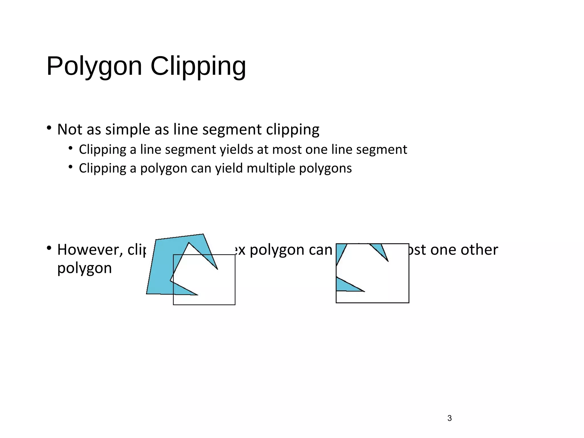
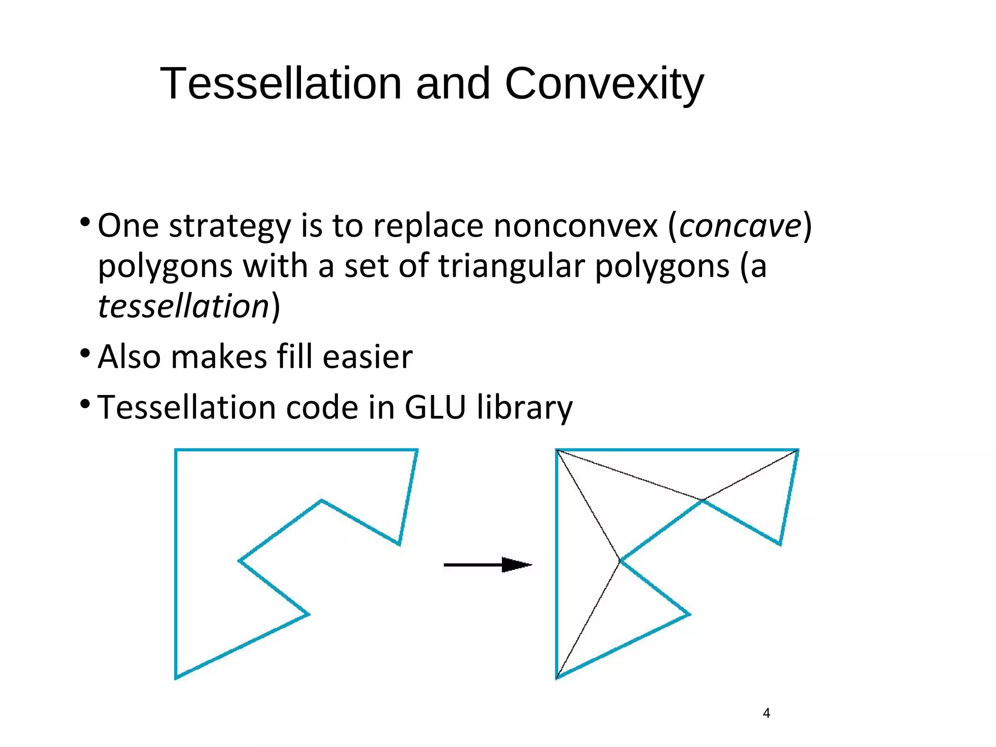
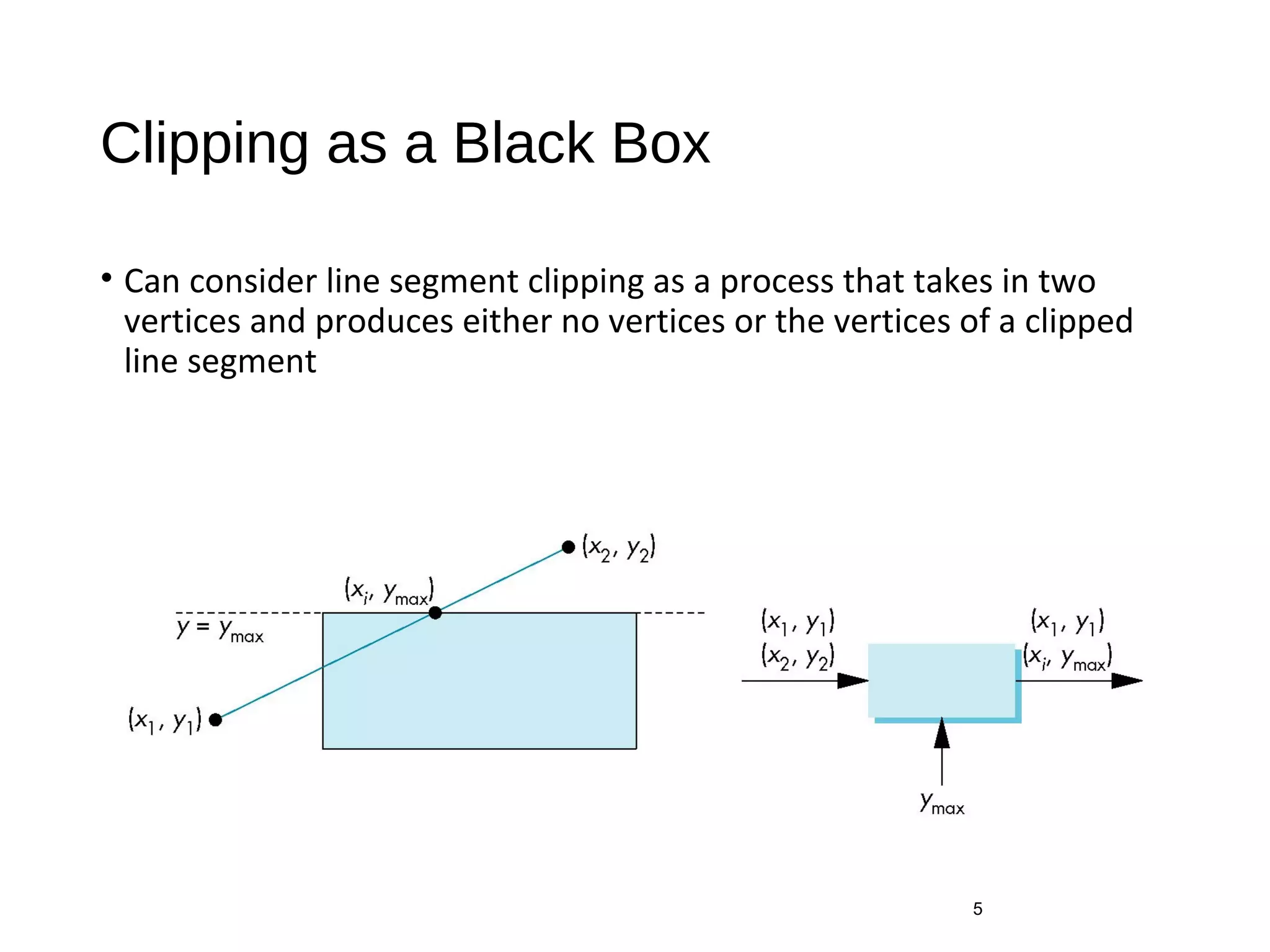
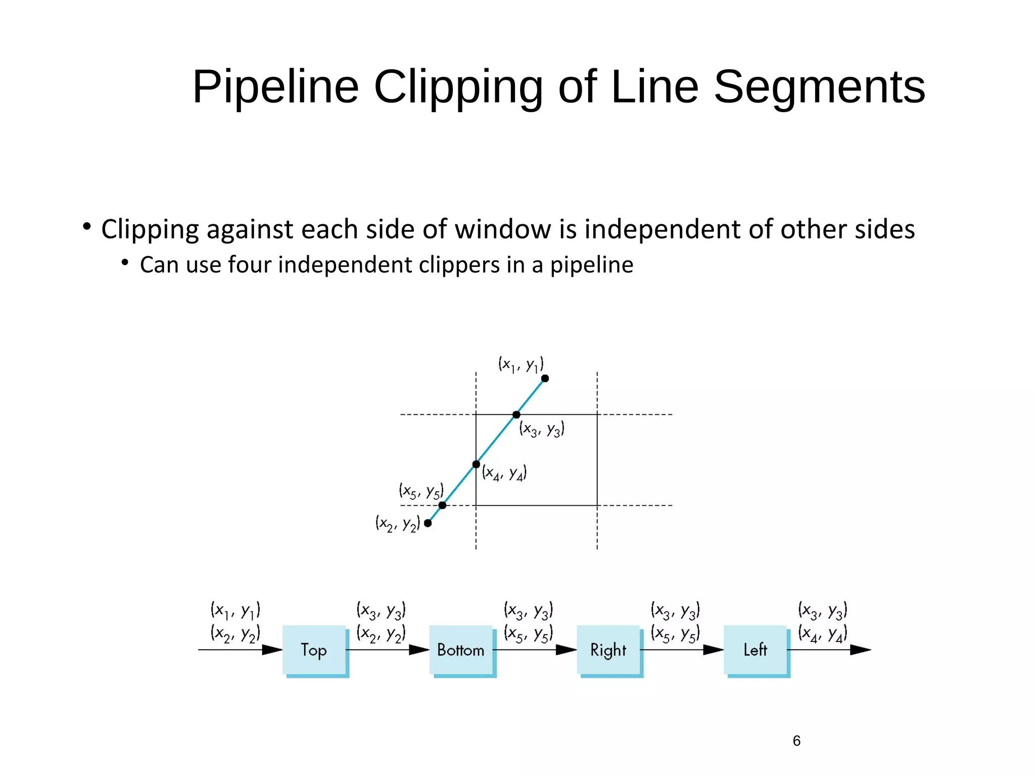
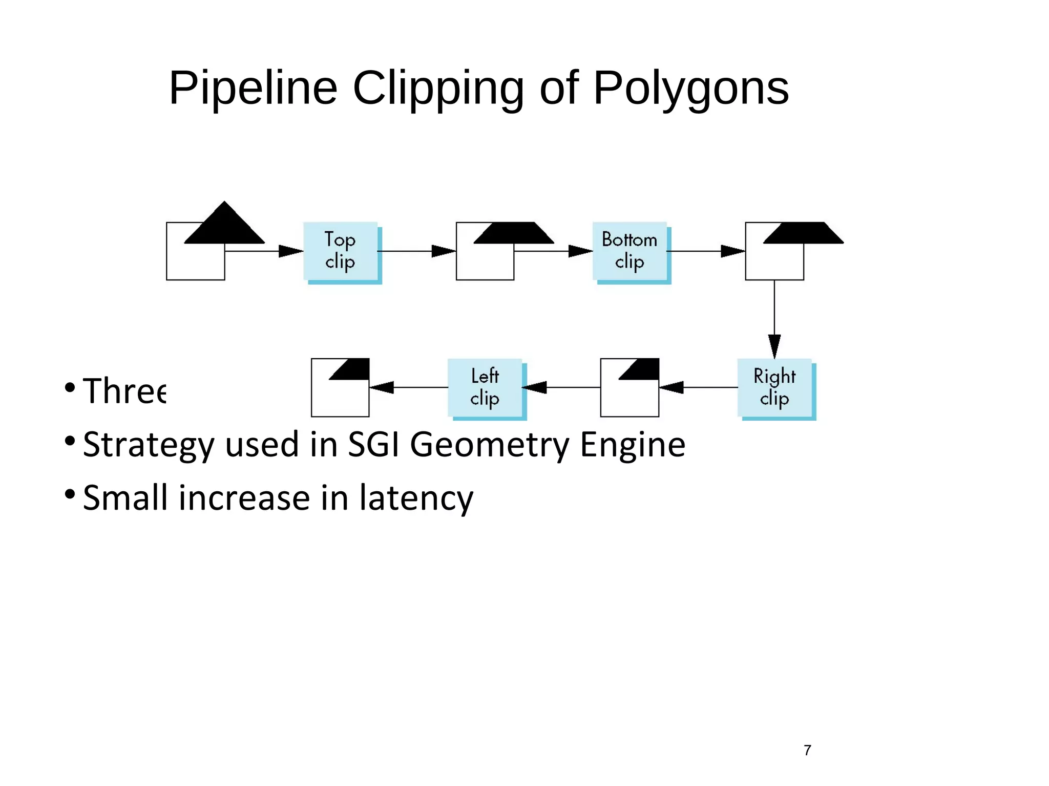
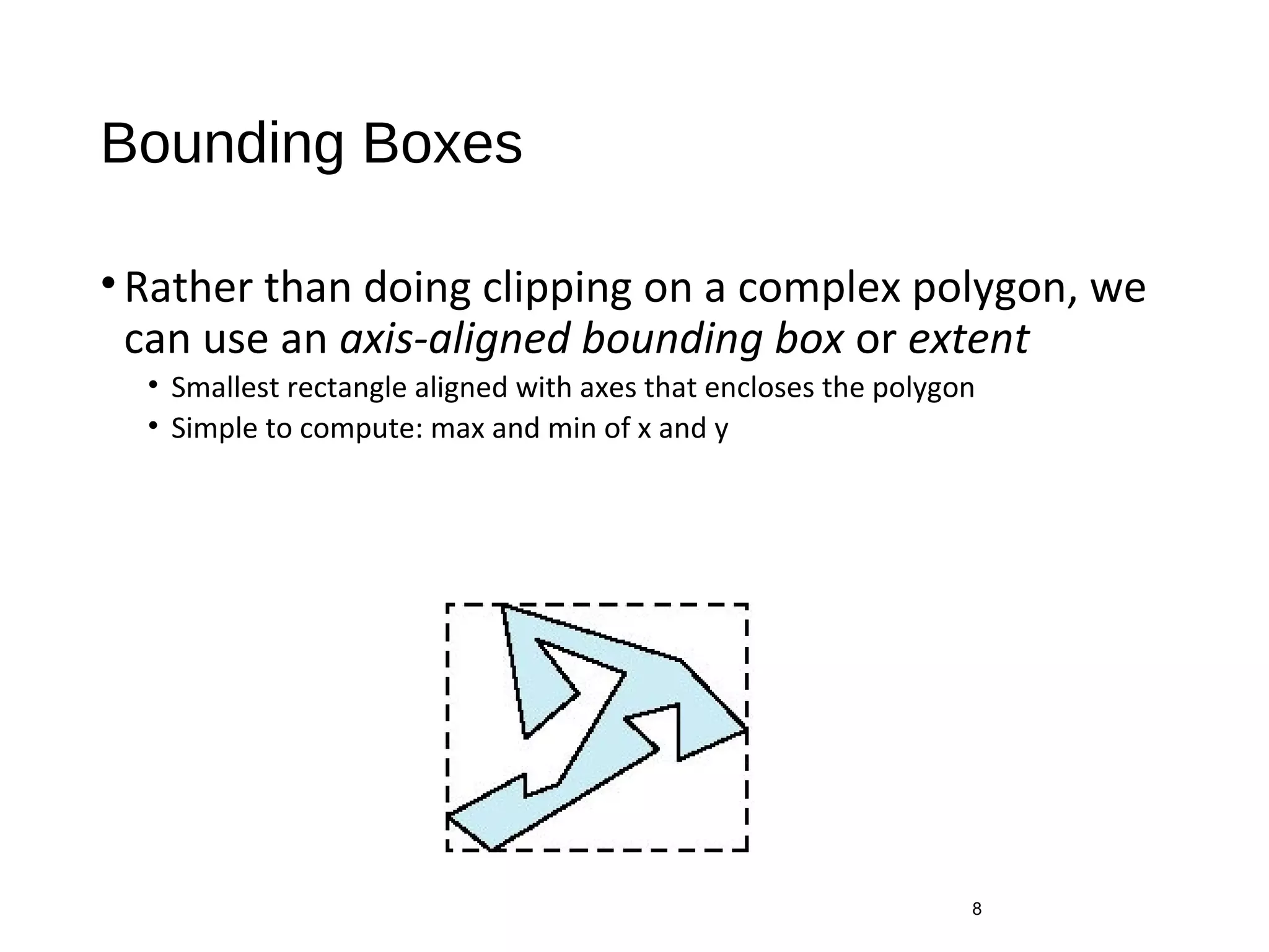
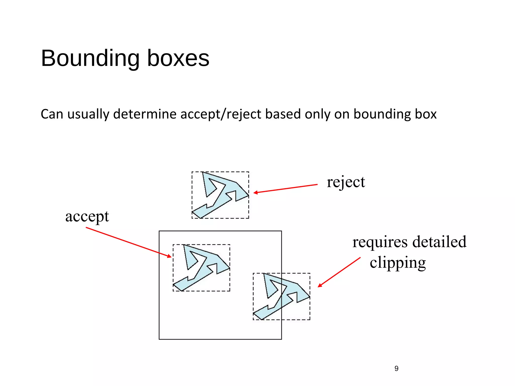
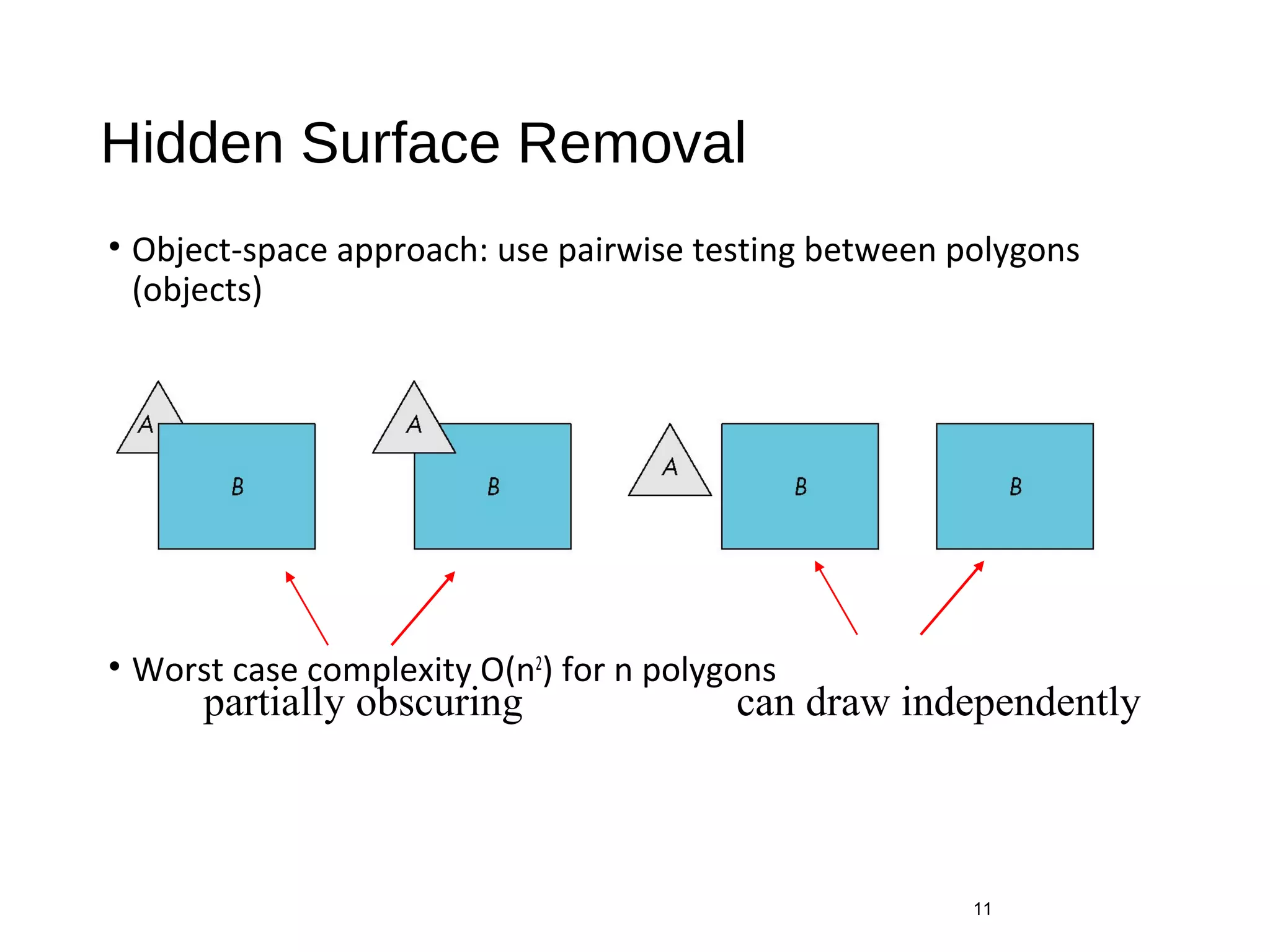
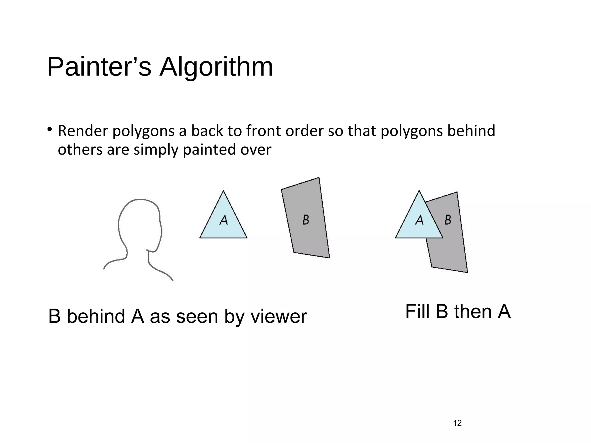
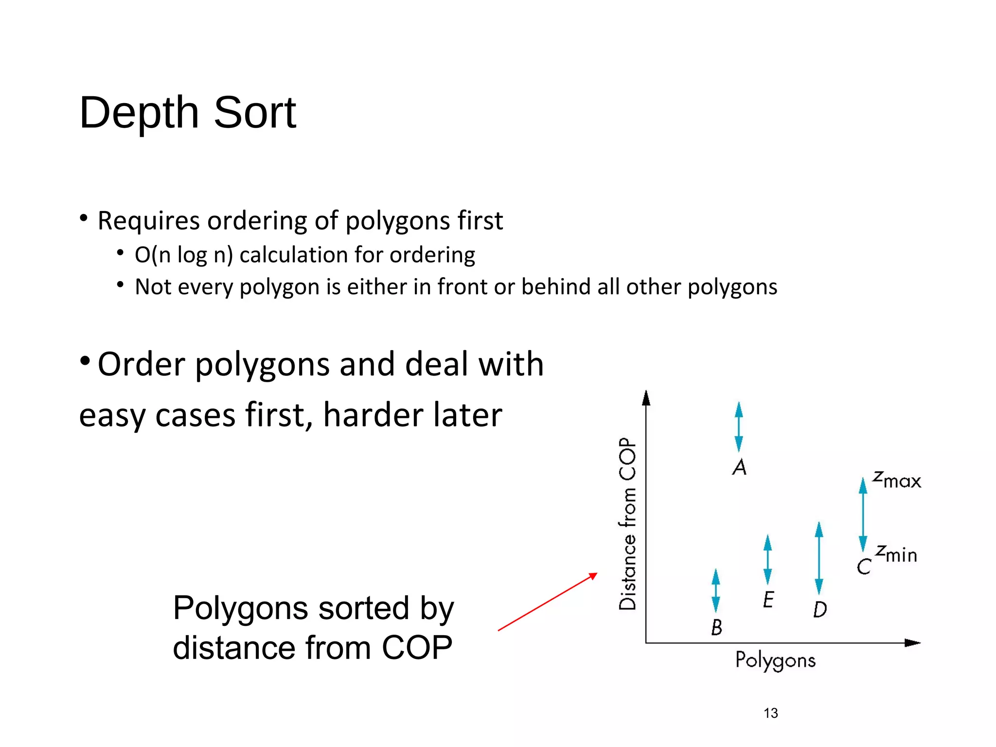
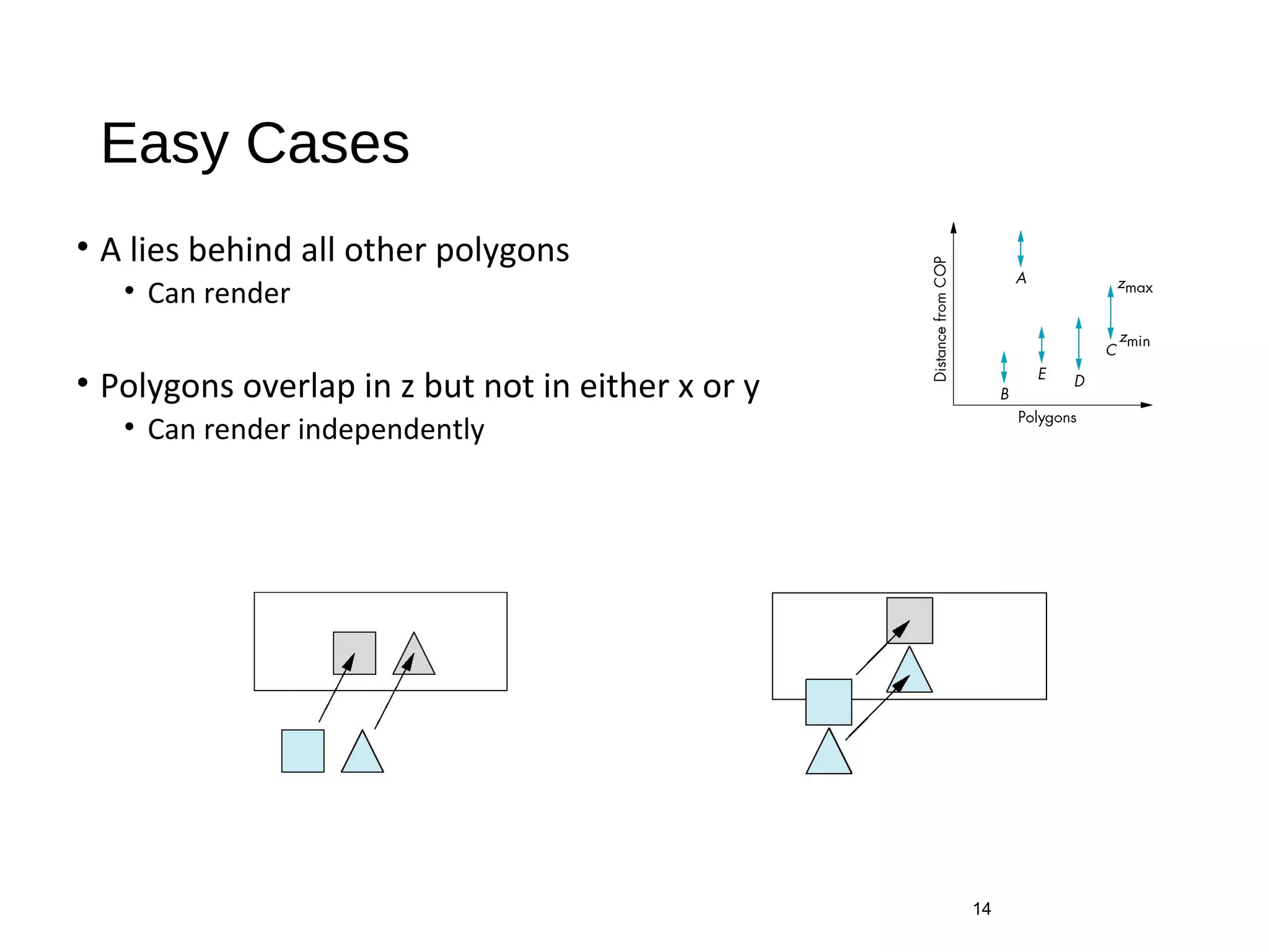
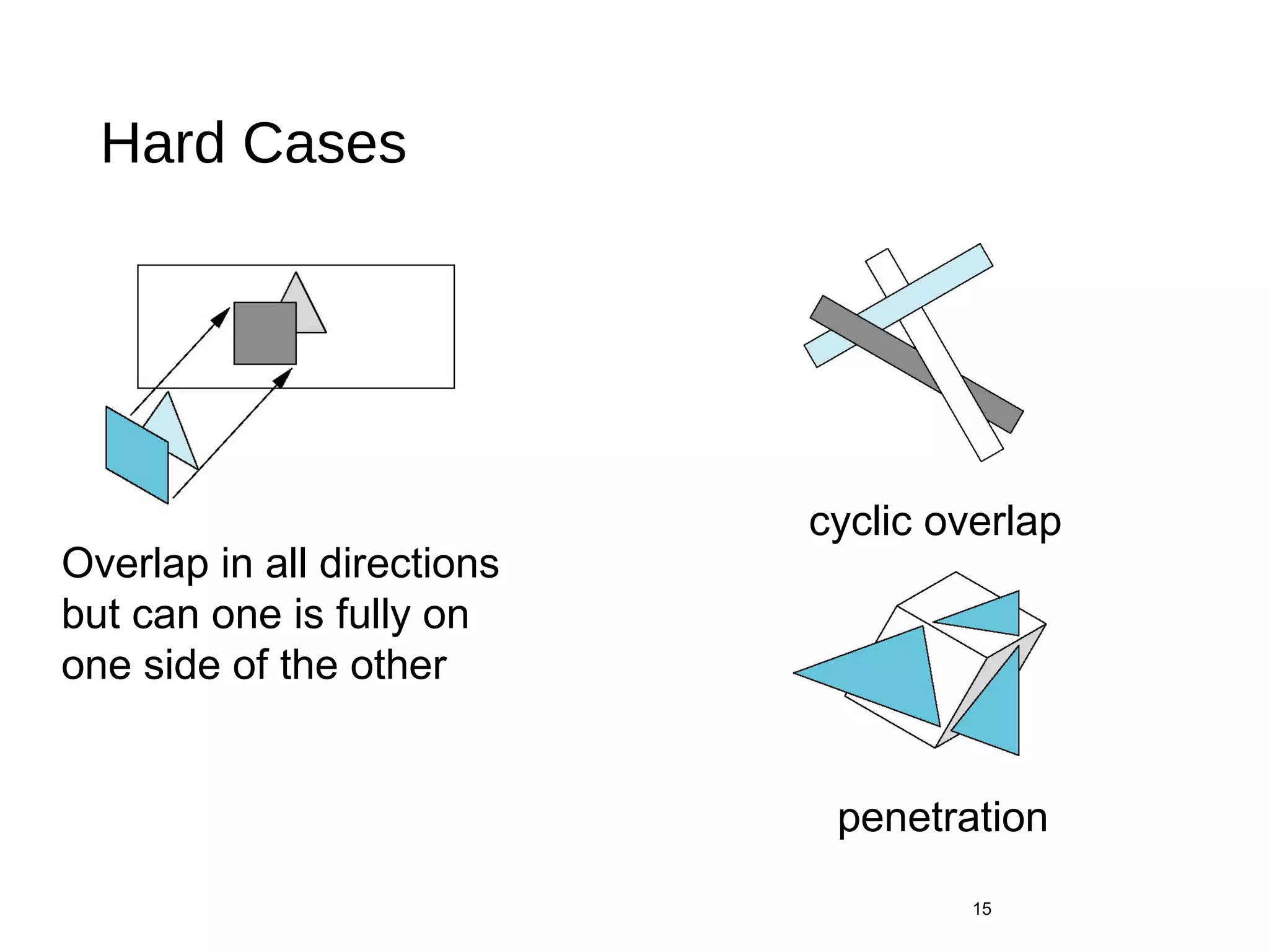
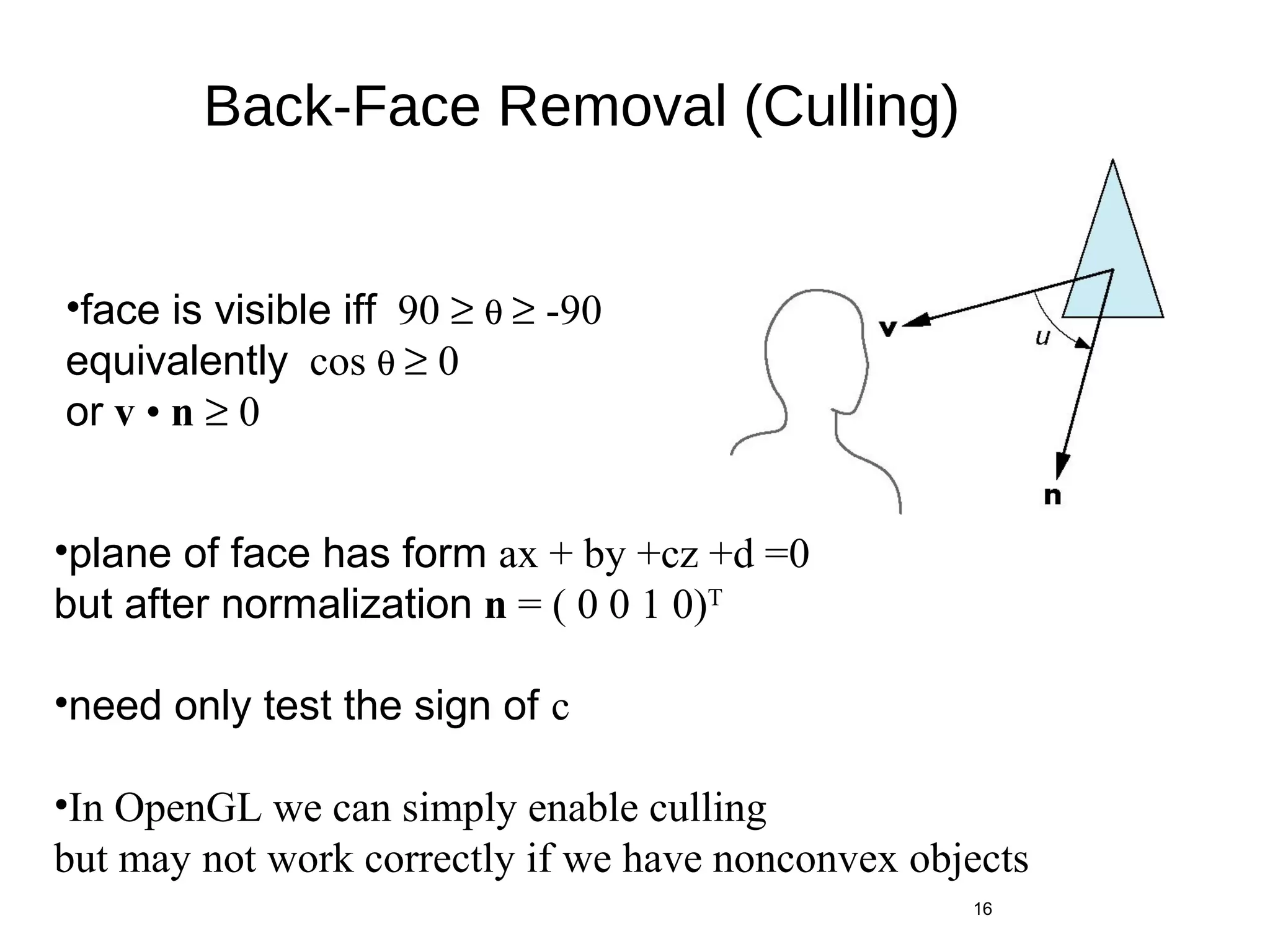
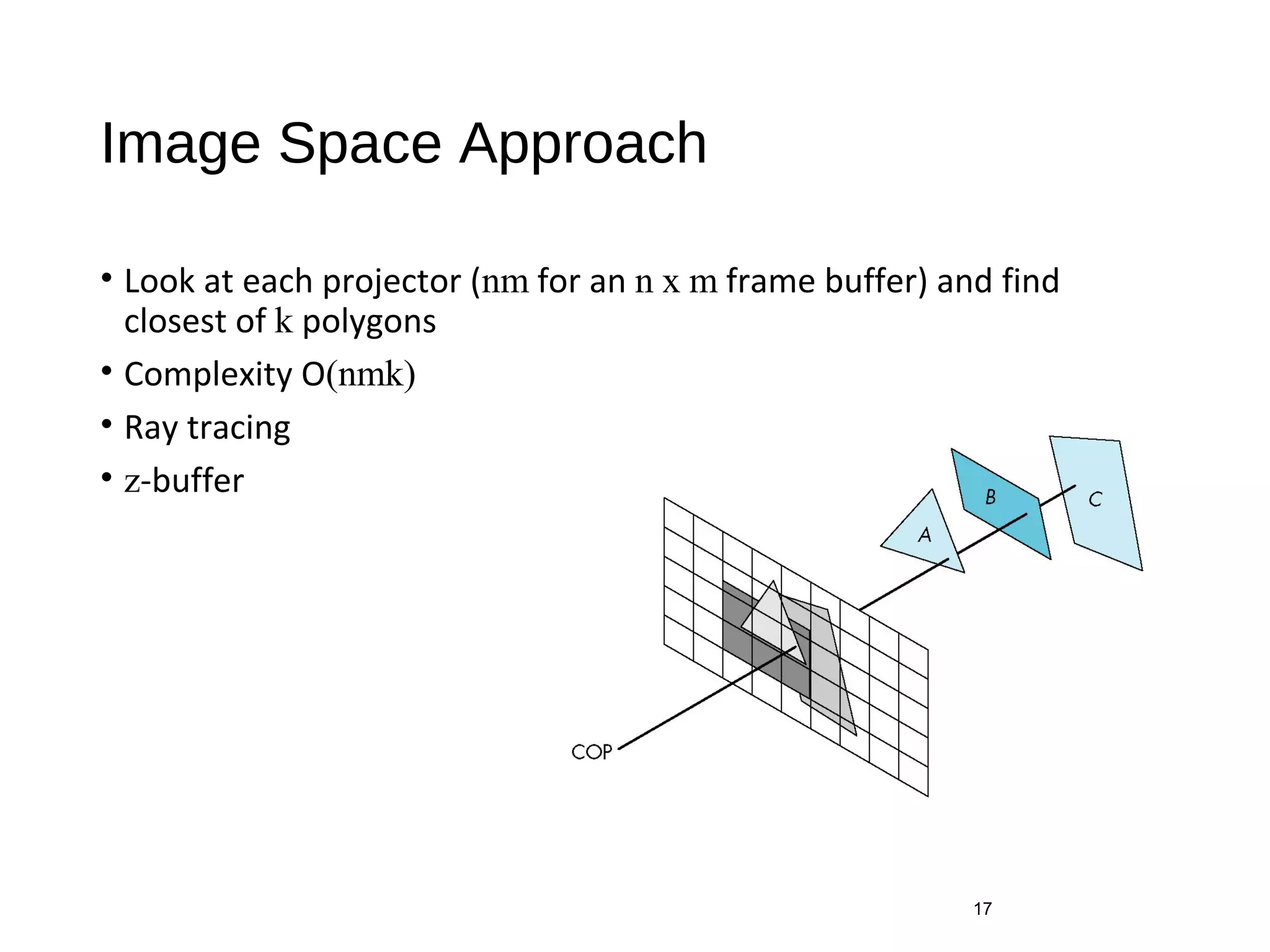
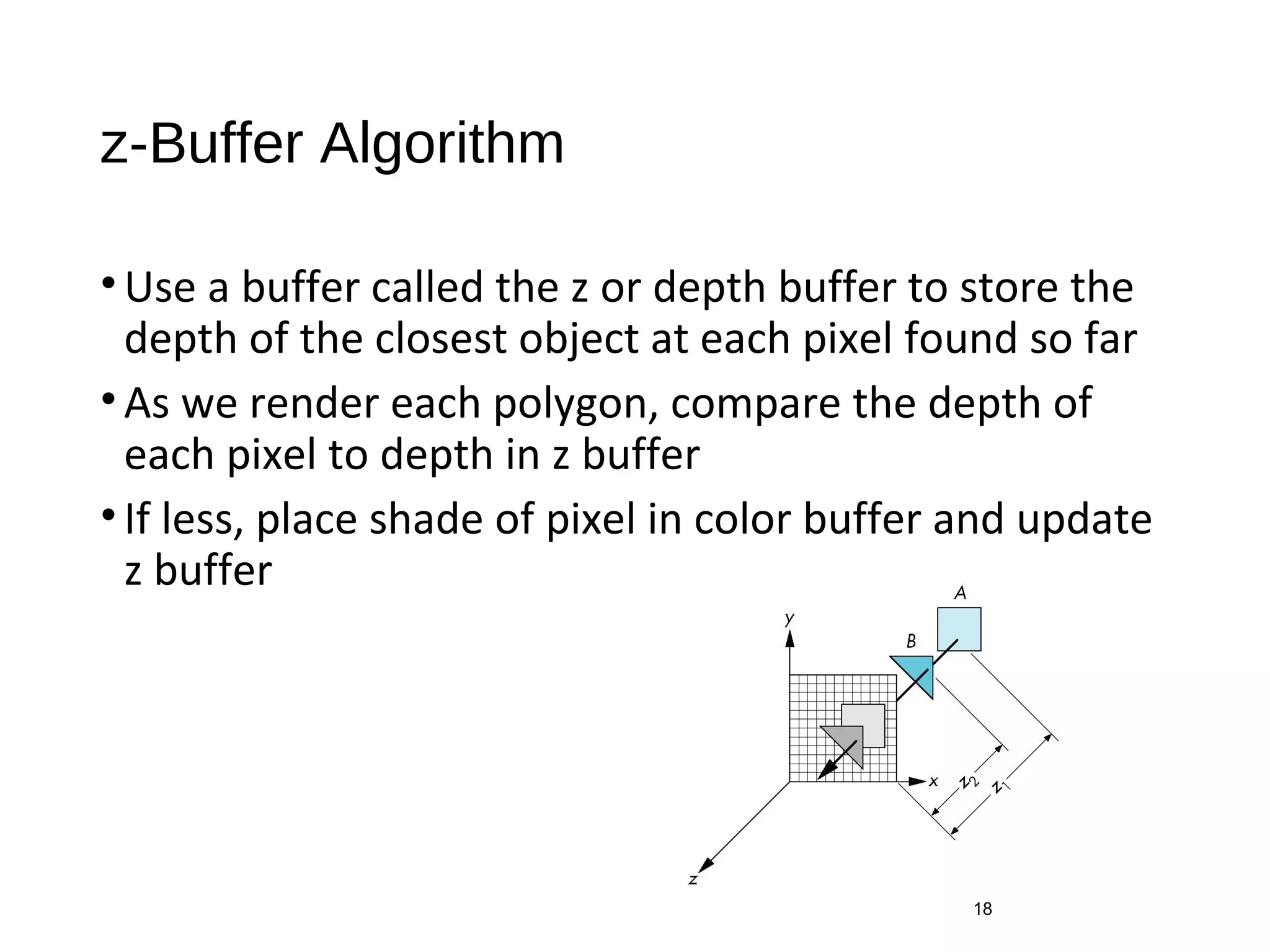
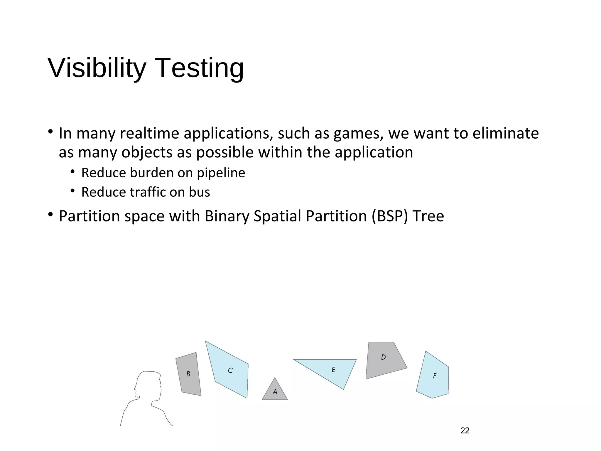
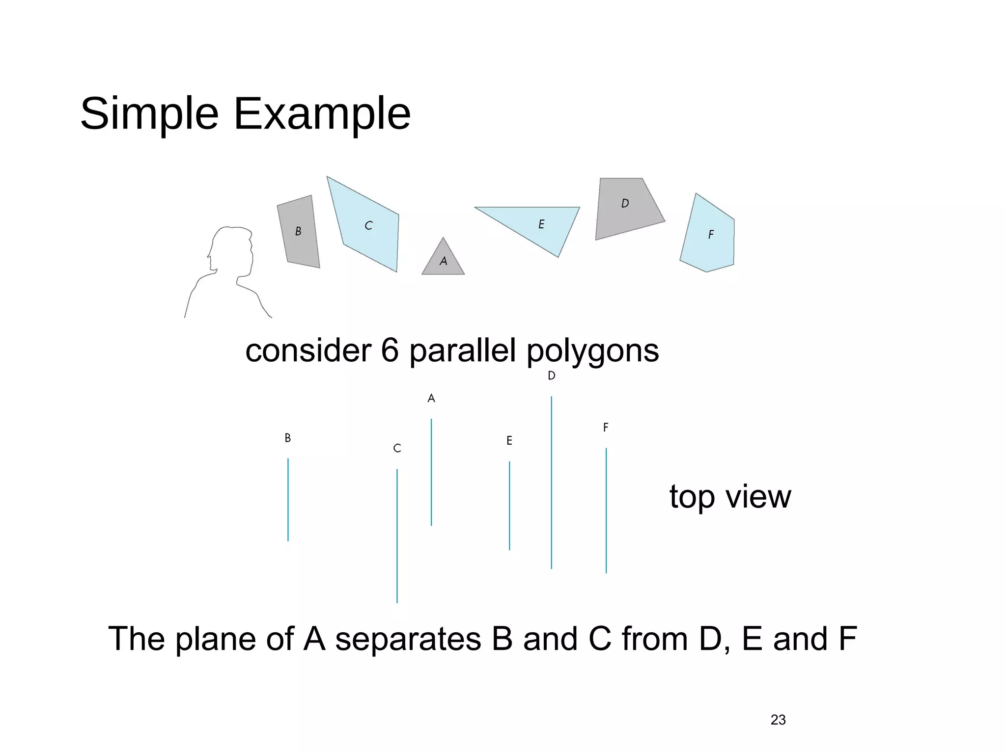
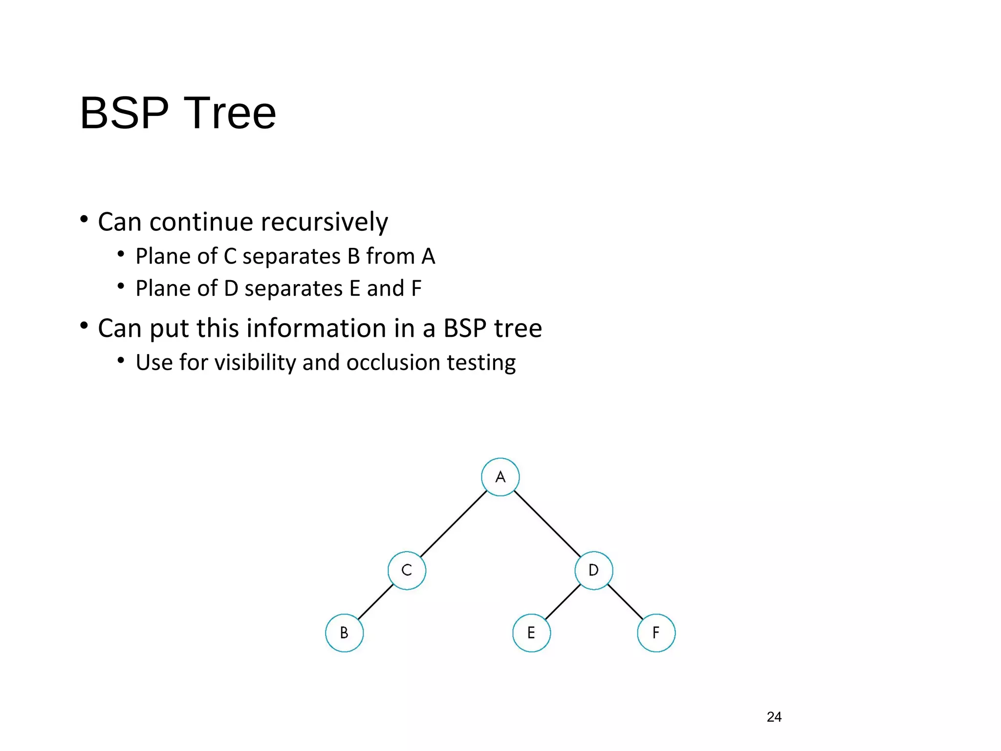
Polygon clipping algorithms can yield multiple polygons when clipping non-convex polygons, but clipping a convex polygon yields at most one other polygon. Tessellation replaces non-convex polygons with triangular polygons. Clipping can be done independently for each side of the window using a pipeline approach. Bounding boxes can determine if detailed clipping is needed. The painter's algorithm and depth sorting are common hidden surface removal techniques. The z-buffer algorithm compares depth values to determine visibility at each pixel. Binary space partitioning trees can partition space hierarchically for visibility and occlusion testing.

1. Implementation II

2. Objectives
• Introduce clipping algorithms for polygons
• Survey hidden-surface algorithms
2

3. Polygon Clipping
• Not as simple as line segment clipping
• Clipping a line segment yields at most one line segment
• Clipping a polygon can yield multiple polygons
• However, clipping a convex polygon can yield at most one other
polygon
3

4. Tessellation and Convexity
•One strategy is to replace nonconvex (concave)
polygons with a set of triangular polygons (a
tessellation)
•Also makes fill easier
•Tessellation code in GLU library
4

5. Clipping as a Black Box
• Can consider line segment clipping as a process that takes in two
vertices and produces either no vertices or the vertices of a clipped
line segment
5

6. Pipeline Clipping of Line Segments
• Clipping against each side of window is independent of other sides
• Can use four independent clippers in a pipeline
6

7. Pipeline Clipping of Polygons
•Three dimensions: add front and back clippers
•Strategy used in SGI Geometry Engine
•Small increase in latency
7

8. Bounding Boxes
•Rather than doing clipping on a complex polygon, we
can use an axis-aligned bounding box or extent
• Smallest rectangle aligned with axes that encloses the polygon
• Simple to compute: max and min of x and y
8

9. Bounding boxes
Can usually determine accept/reject based only on bounding box
9
reject
accept
requires detailed
clipping

10. Clipping and Visibility
• Clipping has much in common with hidden-surface removal
• In both cases, we are trying to remove objects that are not visible to
the camera
• Often we can use visibility or occlusion testing early in the process to
eliminate as many polygons as possible before going through the
entire pipeline
10

11. Hidden Surface Removal
• Object-space approach: use pairwise testing between polygons
(objects)
• Worst case complexity O(n2
) for n polygons
11
partially obscuring can draw independently

12. Painter’s Algorithm
• Render polygons a back to front order so that polygons behind
others are simply painted over
12
B behind A as seen by viewer Fill B then A

13. Depth Sort
• Requires ordering of polygons first
• O(n log n) calculation for ordering
• Not every polygon is either in front or behind all other polygons
•Order polygons and deal with
easy cases first, harder later
13
Polygons sorted by
distance from COP

14. Easy Cases
• A lies behind all other polygons
• Can render
• Polygons overlap in z but not in either x or y
• Can render independently
14

15. Hard Cases
15
Overlap in all directions
but can one is fully on
one side of the other
cyclic overlap
penetration

16. Back-Face Removal (Culling)
θ
16
•face is visible iff 90 ≥ θ ≥ -90
equivalently cos θ ≥ 0
or v • n ≥ 0
•plane of face has form ax + by +cz +d =0
but after normalization n = ( 0 0 1 0)T
•need only test the sign of c
•In OpenGL we can simply enable culling
but may not work correctly if we have nonconvex objects

17. Image Space Approach
• Look at each projector (nm for an n x m frame buffer) and find
closest of k polygons
• Complexity O(nmk)
• Ray tracing
• z-buffer
17

18. z-Buffer Algorithm
•Use a buffer called the z or depth buffer to store the
depth of the closest object at each pixel found so far
•As we render each polygon, compare the depth of
each pixel to depth in z buffer
•If less, place shade of pixel in color buffer and update
z buffer
18

19. Efficiency
• If we work scan line by scan line as we move across a scan line, the
depth changes satisfy a∆x+b∆y+c∆z=0
19
Along scan line
∆y = 0
∆z = - ∆x
c
a
In screen space ∆x = 1

20. Scan-Line Algorithm
• Can combine shading and hsr through scan line algorithm
20
scan line i: no need for depth
information, can only be in no
or one polygon
scan line j: need depth
information only when in
more than one polygon

21. Implementation
• Need a data structure to store
• Flag for each polygon (inside/outside)
• Incremental structure for scan lines that stores which edges are encountered
• Parameters for planes
21

22. Visibility Testing
• In many realtime applications, such as games, we want to eliminate
as many objects as possible within the application
• Reduce burden on pipeline
• Reduce traffic on bus
• Partition space with Binary Spatial Partition (BSP) Tree
22

23. Simple Example
23
consider 6 parallel polygons
top view
The plane of A separates B and C from D, E and F

24. BSP Tree
• Can continue recursively
• Plane of C separates B from A
• Plane of D separates E and F
• Can put this information in a BSP tree
• Use for visibility and occlusion testing
24