How principal components analysis is different from factor

January 28, 2013 ©Arup Guha - Indian Institute of Foreign Trade - New Delhi, India

 Background and Intuition : 3-5

 Principal Components Analysis : 6-15
 Factor Analysis : 16-20

 Comparison between PCA and Factor Analysis : 21-27
 Cases and choice between PCA and Factor Analysis : 28-33


Analyst 1: im confused, should I run pca or factor analysis?
Analyst 2: depends. If you are doing variable reduction or developing a ranking, pca is better. If
you proposing a model for the observed variables, then factor analysis

Analyst1: so there is a difference between the two?
Analyst2: yep

Analyst1: but both give very close communalities
Analyst2: yep but not always

Analyst1: can you tell me the difference between the two?
Analyst2: yep

Analyst1: in non-mathematical terms?
Analyst2: nope. pca is maths and factor analysis is stats. There is no layman analogue of
eigenvectors and eigenvalues that I know of

Analyst1: but if in most cases they are similar, should I bother?
Analyst2: if you trained in maths or stats, yes, or you wouldnt be able to sleep at night. If you are
trained in market research, then no . Serious ans is it depends on data

 n*1 vector of random variables Y
 Say, μi = E(Yi) where i=1,2,…n
 Then var (Yi)=E(Yi- μi)(Yi- μi)… (1)
 And cov(Yi)=E(Yi- μi)(Yi- μj) where i ne j...(2)
 Then (Yi- μi) (Yi- μi)’ gives the variance
covariance matrix where the diagonal
elements are (1) and the off diagonal
elements are (2)

 Think that you are trying to solve this problem
every time you take a photograph - Converting a
3d object into a 2d photograph with maximum
details retained
 If we take a high dimensional data vector in n
space and project into a lower dimensional sub-
space of n-k, k>0 dimensions, and do it such that
the retained variance is maximised, we get PC
 Note, there is no model involved here… just want
to capture the maximum information in the
photograph


 Suppose that x is a vector of p random variables,
and that the variances of the p random variables
and the structure of the covariances or
correlations between the p variables are of
interest
 Say we are lazy and simply don’t want to look at
the p variances and all of the1/2{p(p − 1)}
correlations or covariances
 An alternative approach is to look for a few (<< p)
derived variables that preserve most of the
information given by these variances and
correlations or covariances

 Although PCA does not ignore covariances and
correlations, it concentrates on variances
 The way we would go about finding these PCs is so
that the minimum number of PCs can explain
maximum variance
 The ﬁrst step is to look for a linear function α’1x of
the elements of x having maximum variance, where
α1 is a vector of p constants α11, α12, . . . , α1p
 Next, look for a linear function α’2x, uncorrelated
with α’1x having maximum variance, and so on
 These are the Principal Components

 Consider, for the moment, the case where the vector of
random variables x has a known covariance matrix Σ
 This is the famous variance covariance matrix whose (i,j)th
element is the (known) covariance between the ith and jth
elements of x when i not equal to j, and the variance of the
jth element of x when i = j
 Now two very important results:
1. It turns out that for k = 1, 2, · · · , p, the kth PC is given by
zk = α’kx where αk is an eigenvector of Σ corresponding to
its kth largest eigenvalue λk
2. Furthermore, if αk is chosen to have unit length (α’kαk =
1), then var(zk) = λk, where var(zk) denotes the variance of
zk


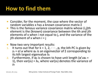
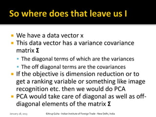
 To derive the form of the PCs, consider ﬁrst
α’1x; the vector α1 maximizes
var*α’1x] = α1Σα1
 It is clear the maximum will not be achieved
for ﬁnite α1 so a normalization constraint
must be imposed
 The constraint used in the derivation is α’1α1
= 1, that is, the sum of squares of elements
of α1 equals 1

 To maximize α’1Σα1 subject to α’1α1 = 1, the
standard approach is to use the technique of
Lagrange multipliers
 Maximise: α’1Σα1 − λ(α’1α1 − 1), where λ is the
lagrange multiplier
 Diﬀerentiation with respect to α1 gives
Σα1 − λα1 = 0,….. (A)
OR, (Σ − λIp)α1 = 0, where Ip is the (p p) identity matrix
 Thus, λ is an eigenvalue of Σ and α1 is the
corresponding eigenvector (from spectral
decomposition, look up)


 Now α1 is supposed to maximise the variance
α’1Σα1
 For that to happen, Σα1 − λα1 =0 must hold
 Or, α’1Σα1 = α’1 λα1 = λ α’1 α1 = λ
 So, the variance, when maximised would equal λ
 Which implies, that if we select the largest
eigenvalue λ and the eigenvector associated with it
α1, we would be maximising the retained variance
and α’1x would be the first PC


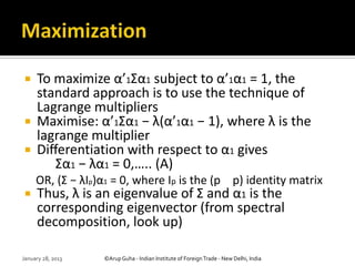
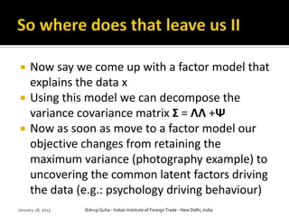
 The second PC, α’2x, maximizes α’2Σα2 subject to
being uncorrelated with α’1x
 Or equivalently subject to cov[α’1x,α’2x] = 0,
where cov(x, y) denotes the covariance between
the random variables x and y
 Solving, we once again come down to maximising
λ but it cant be equal to the largest eigenvalue
since that is already taken by the first PC. So,
λ=λ2, or the second largest eigenvalue of Σ
 And so on


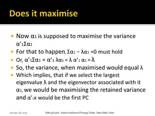
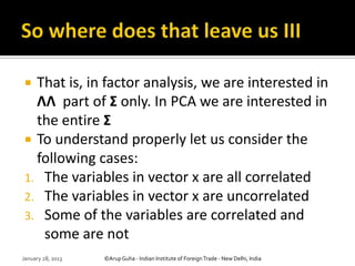
 It can be shown that for the first, second,
third, fourth, . . . , pth PCs, the vectors of
coefficients α1,α2,α3,α4, . . . ,αp are the
eigenvectors of Σ corresponding to λ1, λ2,λ3,
λ4, . . . , λp, the first, second, third and fourth
largest, . . . , and the smallest eigenvalue,
respectively
 Also, var[α’kx] = λk for k = 1, 2, . . . , p.


 Principal component analysis has often been
dealt with in textbooks as a special case of
factor analysis, and this practice is continued
by some widely used computer packages,
which treat PCA as one option in a program
for factor analysis
 This view is misguided since PCA and factor
analysis, as usually defined, are really quite
distinct techniques

 The basic idea underlying factor analysis is that p
observed random variables, x, can be expressed,
except for an error term, as linear functions of m
(< p) hypothetical (random) variables or common
factors
 That is if x1, x2, . . . , xp are the variables and f1,
f2, . . . , fm are the factors, then
 x1 = λ11f1 + λ12f2 + . . . + λ1mfm + e1
 x2 = λ21f1 + λ22f2 + . . . + λ2mfm + e2
 ...
 xp = λp1f1 + λp2f2 + . . . + λpmfm + ep


 λ are the factor loadings
 e’s are the error terms sometimes also called
specific factors. This is because, ej is specific to
xj unlike fk are common to several xj
 fk are the factors common to several x’s
 We will skip the additional details of the
factor analysis model since the objective is to
demonstrate the difference between factor
analysis and pca and not to explain the former

 x = Λf + e (factor analysis model in matrix form)
 Now, going back to the 2 analysts we had met at
the start of this presentation:
 Analyst 2: while factor analysis and pca are both
dimension reduction techniques, factor analysis
attempts to do so by proposing a model relating
the observed to the latent variables. Pca has no
such underlying model
 In other words, the cameraman is just trying to
take the best 2d representation of the 3d world
(pca). He is not trying to fit a model to explain
the world

 Analyst 1: But, since both are trying to do the
same thing, what if pca is used to solve the
factor analysis model? Then there would be
no difference between pca and factor analysis
right?
 Analyst 2: very good point. But pca explains
all the variance and covariance of variance
covariance matrix for a given data. Whereas,
factor analysis explains only the common
variance. Lets get back to models.

 α’kΣαk is maximised by setting α’kΣαk = λk on slide
10
 This maximises var(z=α’kx) but it maximises the
variances along the diagonal of Σ as well as the
off-diagonal covariances or correlations in it
 So PCs explain diagonal elements = variance as
well as off-diagonal = covariance/correlation
elements of the variance-covariance matrix of
the original data matrix x


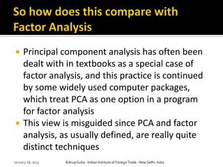
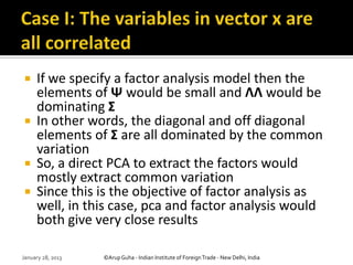
 If you remember the factor analysis model in
matrix form: x = Λf + e
 Along with the following assumptions,
 E[ee] = Ψ (diagonal)
 E[fe] = 0 (a matrix of zeros)
 E[ff] = Im (an identity matrix)
 the above model implies that the variance
covariance matrix would have the form:
 Σ = ΛΛ +Ψ

 Σ = ΛΛ +Ψ
 Now, Ψ is a diagonal matrix, which means that its off
diagonal terms are zero
 So, the contribution of Ψ towards the off diagonal terms of
Σ would be nil
 Note that the relative contribution of ΛΛ and Ψ on
diagonal terms in Σ would depend on the nature of the
variable xj in question
 If xj is highly correlated with all other variables then the
communalities would be large and specific variance or ej
would be low
 On the other hand, if xj is almost uncorrelated with the
other variables then communalities would be low and ej
would be large


 We have a data vector x
 This data vector has a variance covariance
matrix Σ
 The diagonal terms of which are the variances
 The off diagonal terms are the covariances
 If the objective is dimension reduction or to
get a ranking variable or something like image
recognition etc. then we would do PCA
 PCA would take care of diagonal as well as off-
diagonal elements of the matrix Σ

 Now say we come up with a factor model that
explains the data x
 Using this model we can decompose the
variance covariance matrix Σ = ΛΛ +Ψ
 Now as soon as move to a factor model our
objective changes from retaining the
maximum variance (photography example) to
uncovering the common latent factors driving
the data (e.g.: psychology driving behaviour)

 That is, in factor analysis, we are interested in
ΛΛ part of Σ only. In PCA we are interested in
the entire Σ
 To understand properly let us consider the
following cases:
1. The variables in vector x are all correlated
2. The variables in vector x are uncorrelated
3. Some of the variables are correlated and
some are not

 If we specify a factor analysis model then the
elements of Ψ would be small and ΛΛ would be
dominating Σ
 In other words, the diagonal and off diagonal
elements of Σ are all dominated by the common
variation
 So, a direct PCA to extract the factors would
mostly extract common variation
 Since this is the objective of factor analysis as
well, in this case, pca and factor analysis would
both give very close results


 To see this intuitively let us consider the principal
factor analysis, an alternative method to extract
factors
 What it does is, since in factor analysis we are
interested in the common variation only, or
Σ - Ψ = ΛΛ, it applies PCA on Σ - Ψ rather
than on entire Σ
 However, since all variables are correlated, Ψ has
small elements, so the difference between
factors extracted by applying pca on Σ - Ψ vs Σ, is
likely to be minimal


 Again if we consider the factor analysis model, the
diagonal elements of Σ would be dominated by specific
variance from Ψ and the off diagonal elements would
be really small
 Here, an application of pca on Σ would extract PCs that
take care of only specific variance and not common
variation. So they would be very different from the
factors
 Factors drawn through pfa would be different from the
components but the model would not hold since there
is no correlation
 In this case, factor analysis doesnt make sense which
should be clear from the correlation matrix it self

 Consider two variables: xi and xj
 xi is highly correlated with the rest of the variables
 Then in Σ, both the diagonal and off-diagonal elements
of xi are dominated by common variation
 xj on the other hand is not correlated with the rest of
the variables
 In Σ, the diagonal element of xj is dominated by
specific variation from Ψ
 Applying pca on Σ, would once again consider both
common and specific variation making the
components different from factors
 Its better to apply pfa since it would strip Σ of the
specific variance due to Ψ

 Now that we know where the choice between
pca and factor analysis is trivial in practice (they
always make theoretical difference) and where it
is not, how do we choose?
 The answer is the most basic step of statistics
 Know your data
 Or more specifically, know the correlation structure of
your data
 However, since this is difficult and a judgement
call it is always advisable to use non-pca
techniques for factor analysis, lest you come up
with factors that also contain specific variation

How principal components analysis is different from factor

More Related Content

What's hot

Similar to How principal components analysis is different from factor

More from Arup Guha

Recently uploaded

How principal components analysis is different from factor